Library of Layers: Routing Whole Transformer Blocks at Runtime

Review date: 2026-11-11 (UTC)
Author: Zhongzhu Zhou
Paper reviewed: Library of Layers (LoL): Adaptively Ordering Transformer Layers at Runtime
Paper authors: Abdellah Rahmani, Sean McLeish, Ang Li, Sanae Lotfi, Pascal Frossard, Micah Goldblum
arXiv: 2611.03526v1, 2026-11-02

What changes when layers become selectable

A decoder usually has two schedules. Its token schedule comes from autoregression, which produces tokens left to right. Its layer schedule is determined when the network is designed. Library of Layers (LoL) keeps the first schedule and learns part of the second. At each of a fixed number of core depths, a window of tokens uses a single transformer block selected from a shared library. The next depth can pick a different block, or it can reuse the same one. The same stored block can therefore receive very different hidden states across inputs and depths.

I read the paper as an architecture study and an intervention study. The architecture study asks how to let the input choose the order of whole blocks while maintaining causal attention and competitive pretraining loss. The intervention study asks whether replacing the resulting path can control visible solution behavior. The measurements address these questions at different scales and on different training distributions. Results from a model trained to generate five kinds of maze trace should be interpreted separately from results on natural language or from claims about serving.

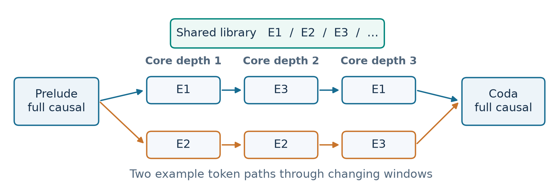
Figure 1. Original schematic from Sections 3.1–3.2. Both illustrated token paths use three blocks, with different order and reuse. Attention and feedforward weights travel together with each expert.

The critical constraint appears as soon as a routed component contains attention. An FFN can process a token on its own, so different tokens can use different FFN experts and still share a common attention layer. A complete block has its own query, key and value projections. If adjacent tokens choose independent blocks, the score between them may compare representations from different learned projections. That product is mathematically defined and could be trained under additional constraints. It changes the attention problem, and the paper reports poor stability and performance for the independent routing setup it tried. LoL groups tokens into windows and limits attention within each group. Window boundaries move across depth, allowing direct token interactions to cross an earlier partition.

Prerequisites and notation

Let $x_i$ be the token at position $i$ and $h_i^{(\ell)}$ the state after core depth $\ell$. The prelude produces $h^{(0)}$, the coda reads $h^{(D)}$, and both use ordinary full causal attention. The library has $L$ experts of compatible width, and the core applies a block $D$ times to each token. At depth $\ell$, each token belongs to exactly one window. Its path follows the expert assigned to its current window at each depth. Since windows move, following a fixed token position through depth and following a fixed window ordinal are distinct indexing conventions. The path-forcing experiment stores choices by window ordinal and depth.

For one attention head of expert $m$, take column vectors $q_i=Q_m u_i$ and $k_j=K_m u_j$, where $u$ denotes the input after normalization and depth modulation. Suppressing position-dependent rotations for this explanation, the query-key score for a pair sharing that expert is

$$s_{ij}^{(m)}=\frac{u_i^\top Q_m^\top K_m u_j}{\sqrt{d_h}} . \tag{1}$$

The head dimension is $d_h$. Softmax over eligible keys turns these scores into weights for the values $V_m u_j$. If the query uses expert $m$ and the key uses expert $r$, the interaction instead contains $Q_m^\top K_r$. The projections can specialize as pairs. A model that freely mixes them needs to learn usable cross-expert interactions or impose alignment through shared projections. LoL preserves the paired basis within each attention operation. Its fixed outer stacks can still communicate across the full prefix using their own common projections.

A residual block maps $h$ to $E_m(h)$ with the skip connection already included. The additive part is $\Delta_m(h)=E_m(h)-h$. Scaling this update leaves the identity path intact. Scaling the full block output would also shrink the skip connection, which would change the behavior every time the selected router probability is small. This distinction matters when many core steps are composed.

Dense, recurrent and sparse models offer three comparisons. A dense stack normally uses a different stored block at each depth. A looped stack reuses a fixed sequence of blocks. An ordinary FFN MoE adds a pool at each depth and chooses a subset for each token, while attention remains tied to the depth. LoL shares a pool of full blocks across depths. Its library size can create forced reuse or room for sparsity, while the router determines which blocks are actually used. Comparing these families requires distinguishing active compute, stored parameters and scheduling.

Shifted windows and a causal router

Deriving the partition

For a document of $n$ tokens, enumerate positions from zero. The window length is $W$, and $S$ is the shift increment across routed depths. For each $\ell$, translate the index by $\delta_\ell$ and integer-divide by $W$.

$$\begin{aligned} \delta_\ell &= ((\ell-1)S)\bmod W,\\ w_\ell(i) &= \left\lfloor\frac{i+\delta_\ell}{W}\right\rfloor,\\ I_{\ell,k} &= \{i:0\le i<n,\ w_\ell(i)=k\}. \end{aligned} \tag{2}$$

The first position of ordinal $k$ is $\max(0,kW-\delta_\ell)$ and its final position is $\min(n-1,(k+1)W-\delta_\ell-1)$. These bounds follow by multiplying the floor inequality by $W$, subtracting the offset, and clipping to the document. There is no cyclic wrap of tokens across the document boundary. Modulo applies to the offset. For $n=8$, $W=4$, $S=2$, depth one groups $[0,3]$ and $[4,7]$. Depth two groups $[0,1]$, $[2,5]$ and $[6,7]$. Depth three restores the first partition. The ordinal of token 4 stays at one in this example, while the set of earlier tokens that it can attend to changes.

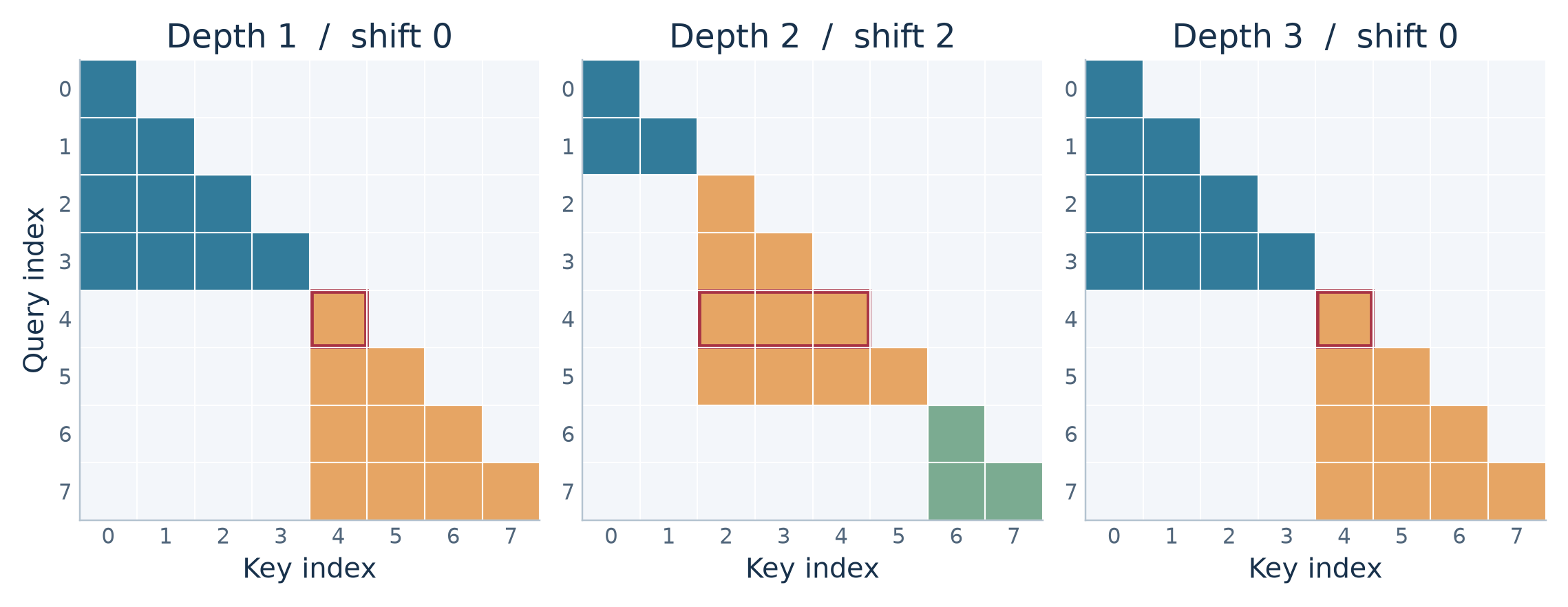
Figure 2. Original redraw of the zero-indexed example in Section 3.2 and paper Figure 2. The row for token 4 acquires direct keys at positions 2 and 3 at depth two.

The allowable keys for query $i$ in the core are all $j\le i$ with the same $w_\ell$. A full window of $W$ tokens contains $1+2+\cdots+W=W(W+1)/2$ causal pairs including self-attention. With an aligned length $n$ divisible by $W$, multiplying by $n/W$ yields $n(W+1)/2$. Full causal attention has $n(n+1)/2$ pairs. At $n=1024$ and $W=128$, the aligned core layer therefore has 66,048 allowed pairs versus 524,800 for full attention. With the 64-token shift, the two half-windows and seven full windows yield 61,952. These counts measure support in the attention mask. Projections, FFN work, data movement and dense outer stacks remain in the cost.

A simple recurrence isolates direct attention reach. Let $a_\ell(i)$ be the earliest position reachable through the residual and core attention edges up to depth $\ell$, starting with $a_0(i)=i$. This deliberately sets aside earlier context already in the prelude and the dependence through routing. At each depth take the minimum over the allowed keys, including $i$ itself.

$$a_\ell(i)= \min_{\substack{j\le i\\w_\ell(j)=w_\ell(i)}}a_{\ell-1}(j). \tag{3}$$

At token 4 the earliest indices after depths one, two and three are 4, 0 and 0. In depth two, position 4 can read position 2, whose depth-one state already reads position 0. When $S=0$, this direct path cannot cross the original window boundary at any depth. Even then, the router and the fixed full-attention stacks can transmit earlier information through other channels. A reachability edge states where information can flow. Learned weights determine how much signal it actually carries.

Deriving prefix-only routing

For a window $k>0$, compute each earlier window mean $\mu_j$ from the input to this routed depth. Average those means with equal window weight. For window zero, use the mean of the first-token state and a learned depth vector $e_\ell$.

$$\begin{aligned} \mu_j &= \frac{1}{|I_{\ell,j}|}\sum_{i\in I_{\ell,j}}h_i^{(\ell-1)},\\ r_0 &= \tfrac12\left(h_0^{(\ell-1)}+e_\ell\right),\\ r_k &= \frac{1}{k}\sum_{j=0}^{k-1}\mu_j\qquad(k>0). \end{aligned} \tag{4}$$

The equal-window average has a subtle consequence when the first window is clipped. In the shifted eight-token example, the last window reads the means of $[0,1]$ and $[2,5]$. Each token in the short window has coefficient $1/4$, and each in the full window has coefficient $1/8$. Pooling the entire prefix uniformly would give $1/6$ to all six tokens. Equal weighting of windows follows the paper. Uniform token weighting is a plausible alternative that would change routing even with the same weights and masks.

Every token contributing to $r_k$ for $k>0$ precedes the first token in $I_{\ell,k}$. If the previous depth states depend only on their respective prefixes, the selected expert and gate depend only on a prefix available to every token in the window. The first window gets the state of position zero, which is available to all its queries. With the causal mask inside the selected block, an output at position $i$ depends only on $x_{\le i}$. The prelude provides the base case and the coda preserves the induction. This argument describes the standard language-model forward pass with fixed model parameters and any routing noise held fixed per corresponding window. The synthetic task gives the router an explicit condition under its separate data protocol.

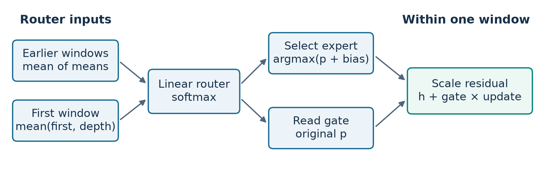
Figure 3. Original schematic of Section 3.2 and Appendix A. Routing uses previous-depth states. A causal attention mask alone would leave a leakage path if the router pooled future tokens in the current window.

A useful deployment property follows. At a fixed depth, each window has a stable identity and gate as the context grows. Earlier windows are already complete when the new window opens. The first token and the depth vector are stable for window zero. The cost of preserving that property depends on how the serving runtime maintains per-depth window boundaries and summaries. If it restarts window ordinals independently for each decode chunk, it changes the modeled function. With packed documents, resetting and isolating routing summaries at document boundaries is necessary to obtain per-document prefix independence. Appendix A explicitly documents blocked attention; the routing boundary should be tested separately when evaluating a packed execution.

Routing gradients, load balance and depth conditioning

The router is linear on $r_k$. Write $z=A r_k+c+\epsilon$ for the logits, where $\epsilon$ denotes the Gaussian training perturbation, and $p=\operatorname{softmax}(z)$. Appendix A describes a selection bias $b_m$ applied in probability space. After selection, the gate uses the original probability of the selected expert.

$$\rho=\operatorname*{argmax}_{m}(p_m+b_m),\qquad \alpha=p_\rho,\qquad y_i=h_i+\alpha\bigl(E_\rho(h_{I})_i-h_i\bigr). \tag{5}$$

This separates exploration and expert usage from residual magnitude. For example, $p=(0.45,0.40,0.15)$ and $b=(0,0.08,0)$ select expert two with gate $0.40$. Adding the bias to the logits before softmax is a different operation. Using $0.48$ as the gate is also a different forward pass. Appendix B compares auxiliary-loss balancing with loss-free balancing and reports a lower final cross-entropy for the latter in the studied run. The result motivates the design but does not determine the optimal bias update schedule for every library or batch.

For a local derivative, freeze $\rho$ and hold the layer input fixed. If $g_i=\partial\mathcal L/\partial y_i$, each token sends a scalar contribution to the shared gate via $g_i^\top\Delta_{\rho,i}$. Differentiate the normalized exponential $p_\rho=\exp(z_\rho)/\sum_m\exp(z_m)$. The numerator contributes only for $j=\rho$, and the denominator contributes $-p_\rho p_j$ for each logit $z_j$. Combining the chain rules gives

$$\begin{aligned} \frac{\partial \mathcal L}{\partial \alpha} &=\sum_{i\in I}g_i^\top\Delta_{\rho,i},\\ \frac{\partial p_\rho}{\partial z_j} &=p_\rho\left(\mathbf 1_{j=\rho}-p_j\right),\\ \frac{\partial \mathcal L}{\partial z_j} &=\left(\sum_{i\in I}g_i^\top\Delta_{\rho,i}\right) p_\rho\left(\mathbf 1_{j=\rho}-p_j\right). \end{aligned} \tag{6}$$

This derivative is one branch of the network gradient. The sum aggregates the whole window and may reinforce or cancel across tokens. It does not carry a gradient for the counterfactual expert that would be chosen on the other side of an argmax boundary. If the selected gate saturates at one, the softmax derivative tends toward zero. If a balancing bias selects an expert with a tiny $p_\rho$, the residual update and that branch of the router signal become small. The paper uses logit noise to sample a wider set of experts while training. A top-$k$ mixture would furnish direct signals for more expert outputs but would use more block applications per token and require each active attention path to remain internally consistent.

Each shared block also receives depth-specific feature-wise linear modulation (FiLM). For either sublayer $s$ in attention or FFN, the normalized input is replaced by

$$u_{\ell,s}=\gamma_{\ell,s}\odot \operatorname{Norm}_{s}(h)+\beta_{\ell,s}. \tag{7}$$

A change in $\ell$ changes the input to the same matrix multiplications. For example, one feature’s downstream weight is effectively multiplied by its entry in $\gamma_{\ell,s}$, and $\beta_{\ell,s}$ shifts the resulting projection. This lets a shared expert specialize softly by depth. A complete untied block would allow more expressive depth-specific changes, while giving up the storage benefit. Fully depth-agnostic recurrence would preserve more sharing but remove that adaptation. FiLM is also a confound for interpreting interventions as swapping abstract algorithms. The same ID can implement different effective transformations at different depths. Appendix B.2 and Figure 9 address attention patterns and router tying, respectively. Router tying still permits variation from different hidden states and the first-window depth vectors.

Algorithm 1. Forward pass with shifted window routing

This is a reader-oriented form of paper Algorithm 1 and Appendix A for a standard document. Accumulate the sum of preceding window means; computing the same prefix sum from scratch for every window would introduce unnecessary repeated work. The independent windows can be batched after routes are known.

01  Apply the causal prelude to the token sequence; store H.
02  For each core depth l from 1 through D:
03      Partition indices using offset ((l-1) * S) mod W.
04      Compute each window mean from the unchanged H.
05      For each window k, form r using the earlier means.
06          For k=0, use (H[0] + depth_vector[l]) / 2.
07          Compute router probabilities (noisy in training).
08          Choose the argmax of probability plus selection bias.
09          Apply that expert with depth-conditioned normalization.
10          Within the block, attend only to causal keys in k.
11          Write next_H[k] = H[k] + probability * (block[k] - H[k]).
12      Replace H with next_H after all windows at this depth.
13  Apply the causal coda and vocabulary readout.

Line 4 must read the input states of the current core depth, including when windows are processed in parallel. If later windows instead summarize earlier windows after their blocks are applied, the computation introduces an additional same-depth dependency. It can remain left-to-right causal, but changes the architecture and can serialize prefill. With the paper’s schedule, summarization is parallel, prefix means can be formed by a scan, and per-expert execution can group ready windows. Inference may drop the training noise without changing the causal proof. Forcing a path supplies both an expert ID and a gate at line 8 and line 11, while the attention mask and depth index stay as before.

Capacity, compute and the growing schedule

Stored blocks, uses and observed sparsity

For a particular token path, let $U$ be the number of distinct expert IDs across its $D$ positions. The pigeonhole principle bounds it by $\min(L,D)$. Count the repeated applications after the first use of each block and the untouched library entries:

$$1\le U\le\min(L,D),\qquad N_{\rm repeated}=D-U,\qquad N_{\rm unused}=L-U . \tag{8}$$

At $L=2$ and $D=16$, at least 14 applications repeat an ID. At $L=24$ and $D=16$, at least eight library entries are unused on every token path. A path that alternates just two experts has 22 unused entries in the second case. Both scenarios apply the same number of core blocks per token. As a separate illustration, for independent uniform routing at each depth, a given expert is absent with probability $(1-1/L)^D$. Sum the indicators of expert presence to obtain the expected number of distinct blocks.

$$\mathbb E[U]=L\left[1-\left(1-\frac{1}{L}\right)^D\right]. \tag{9}$$

For $D=16$, this null model gives approximately 7.06 distinct experts at $L=8$ and 11.85 at $L=24$. Real routes are correlated and constrained by hidden states and balancing. A large difference from this curve could arise from deliberate reuse, specialization by depth or a concentrated router. Distinguishing them requires a joint measurement of use by depth, within-path diversity and across-window load. A library can be underused on each individual path while every expert receives training across a batch.

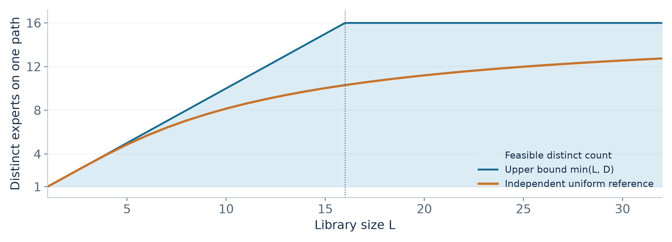
Figure 4. Original analytical plot for depth 16. The shaded region is the feasible range. The independent uniform model gives a reference curve for diversity.

If an expert holds $P_E$ parameters, core parameter storage is approximately $LP_E$ plus the router and FiLM overhead. An application touches one expert per token and invokes its projections and feedforward network, so active work from block applications scales roughly with $DP_E$ per token under a matrix-dominated approximation. This product counts repeated parameter use. It is neither a count of unique weights read from device memory nor a timing estimate. At fixed width, computing all scores costs on the order of $K_\ell dL$ for $K_\ell$ windows, before selection and dispatch. At large $L$ the router can become material, and fragmented batches can make expert GEMMs inefficient. Window routing reduces the number of routing decisions relative to per-token routing, while whole-block dispatch couples attention with the selected expert.

Growing the core during training

The core starts shallow and adds routed depths during training. The paper reports a schedule described as one minus square root over the growing phase for the 1B math runs, occupying 75% of training. Appendix Figure 7 compares fixed depth 16 to growth from 1 to 16, and additionally plots a final-eight backpropagation variant with full backpropagation for first windows. On a step axis a shallower model may be worse while it is still growing. On a FLOP axis it can process more data early. The paper observes a modest terminal loss difference in the growth ablation, so comparisons should specify both the training axis and the attained depth.

For a transparent budgeting example, let $T$ be the number of training tokens, $F_o$ the approximate per-token cost of the fixed stacks and $F_b$ the incremental per-token cost of one core application. Sum over tokens, grouping by their scheduled depth $D_t$. Compared with training at a fixed final depth $D_*$, the fractional saving in this simplified model is

$$\begin{aligned} F_{\rm grow}&\approx T(F_o+F_b\overline D),\\ 1-\frac{F_{\rm grow}}{F_{\rm fixed}} &\approx \frac{F_b(D_*-\overline D)}{F_o+F_bD_*}. \end{aligned} \tag{10}$$

If the outer stacks cost eight block-equivalents, the final core depth is 16 and the mean core depth is 10, the illustrative saving is $6/24=25\%$. This is a budgeting example, not a measurement of the paper’s schedule. The cost of optimizer updates on stored experts, expert parallel communication, attention, activation storage and truncation can all break proportionality. Depth growth also changes optimization: it gives the router fewer decisions early and exposes later depth-specific features to fewer tokens. Separating this curriculum effect from a generic cheaper attention mask or a different number of training tokens requires matched controls.

What it means to force a strategy

The intervention begins with a controlled training signal. In the synthetic tasks, each problem is paired with traces from five specified strategies. During training, the strategy description is visible to the router and masked from the rest of the network. The loss covers the trace and answer. Sudoku puzzles retain 30–36 digits and are selected to be solvable by all five methods. Their step formats distinguish naked singles, hidden singles, crosshatching, propagation and DFS backtracking. Mazes use an $8\times8$ loop-free grid with a path of at least 12 cells. The generator also selects cases where BFS explores at least three off-path cells and DFS backtracks, so the requested exploration order has a chance to be observable. Appendix C gives about 20M deduplicated sudoku sequences and 36M maze sequences over 7.2M mazes, with about 10B training tokens per task.

Maze traces all use cell identifiers. BFS and DFS can produce the same final path through a tree, yet BFS discovers a frontier in breadth order and DFS can revisit a parent while backtracking. A* uses a Manhattan heuristic. Bidirectional BFS alternates frontiers, and dead-end filling removes leaves. Figure 19 makes the target-vs-trace distinction concrete: several strategies end with the same list of answer cells and differ strongly in the trace before it. This controls a surface-format shortcut present in sudoku. It still leaves a highly structured generator and a unique correct final path. The task asks whether the model can produce strategy-specific traces under these controls.

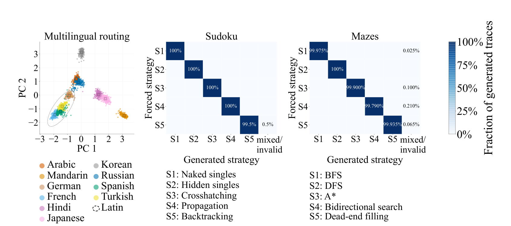
Figure 5. Cropped from paper Figure 3, p. 6, with the three panels intact. The left panel is a PCA visualization. The confusion matrices summarize the paper’s strategy categories under path forcing.

Constructing a path from validation probabilities

Let $s$ index a strategy and $V_{s,\ell,k}$ be its validation examples with an observation at window ordinal $k$ and routed depth $\ell$. The teacher-forced forward pass supplies probabilities over all experts at that position. The paper averages the probabilities and freezes the largest coordinate and its value.

$$\begin{aligned} \bar p_{s,\ell,k,m} &=\frac{1}{|V_{s,\ell,k}|} \sum_{x\in V_{s,\ell,k}} p_{\ell,k,m}(x),\\ \rho^*_{s,\ell,k}&=\operatorname*{argmax}_m\bar p_{s,\ell,k,m},\\ \alpha^*_{s,\ell,k}&=\bar p_{s,\ell,k,\rho^*_{s,\ell,k}}. \end{aligned} \tag{11}$$

The word mode is convenient here and somewhat misleading. A coordinate-wise maximum of averaged probabilities can differ from the most frequent discrete ID, especially when load-balancing bias is present during selection. Even without bias, consider three observations with two experts and first-expert probabilities $0.51,0.51,0.01$. The first expert wins twice and has mean $0.3433$. The second expert has mean $0.6567$ and is forced with that gate. Moreover, marginal winners need never co-occur on a single real path. A path built from them is a template for the intervention. It need not approximate the most likely joint execution.

Algorithm 2. Extract and apply a forced path

01  For each strategy, run labeled validation traces teacher-forced.
02  Accumulate pre-bias probabilities by depth and window ordinal.
03  For each observed cell, divide by its observation count.
04  Store the winning expert ID and its mean probability.
05  On a fresh problem, replace the strategy field with neutral filler.
06  At each routed depth/window, supply the stored ID and gate.
07  Generate the trace and answer autoregressively.
08  Score requested strategy, legal trace and final answer separately.

Line 2 uses observations from complete validation trajectories. At test time the stored template can be applied without seeing any future generated token. This distinction prevents a misreading of teacher forcing as test-time leakage. It also makes template support important. The appendix shows unobserved positions and says maze dead-end filling reuses the W2 expert sequence if W3 is reached. That is evidence of one fallback policy, not support for arbitrary trace lengths. A clean extension would track count, uncertainty and fallback behavior per cell, and report accuracy by whether the rollout stayed within supported cells.

Reading strategy adherence and correctness separately

The main text reports essentially perfect strategy adherence under forced routes, with the largest sudoku miss in the backtracking condition and the largest maze miss in bidirectional search. The appendix bars make it possible to read finer outcomes. In paper Figure 14, the S2 hidden-singles route shows 100% requested strategy, 96.5% trace rule-faithful and 98.5% answer correct. S5 shows 99.5%, 97.5% and 99.0%, respectively. The paper’s description of a correct trajectory requires legal steps, requested strategy and a correct solution. These marginal bars do not reveal the exact intersection. For S2, the reported rule-faithful and answer-correct rates alone constrain their intersection to 95.0–96.5% by the union bound. The main heatmap should therefore be read with its generated-strategy axis in view.

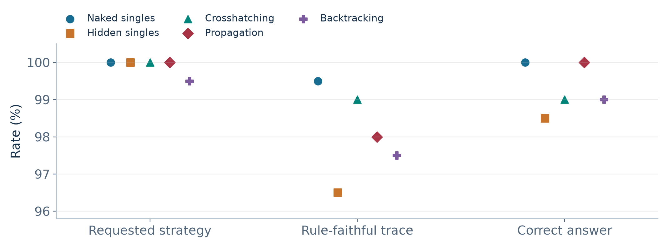
Figure 6. Redrawn from paper Figure 14. The vertical axis is truncated to show small differences. The three columns measure different outcomes under the appendix caption’s forced-routing condition.

There is a protocol labeling ambiguity worth preserving. Sections 4.1.3–4.1.4 refer to appendix Figures 14 and 18 when discussing evaluation with the strategy description in context, while both appendix figure captions say forced routing. The main Figure 3 and the protocol description directly support the forced-routing result. The appendix bars are identified by their own captions here, and I do not use them to estimate a forced-versus-prompted performance gap.

Agreement with the template at each depth is a different quantity again. Appendix Figures 12 and 16 compare the chosen expert with the forced template. In sudoku’s first window the mode IDs match across strategies in Figure 13, while agreement can fall to zero at some depths in Figure 12. The strategy-specific paths diverge in later windows. A successful forced trajectory is compatible with low agreement in some cells. Several routes may be functionally similar, and changing the gate at the same time can compensate. I would compare route-only, gate-only and joint interventions before attributing control to the order of expert IDs.

Reading routing features in natural language

The multilingual run trains a 360M-scale model on a balanced mixture of ten FineWeb-2 languages for 10B tokens. For each sampled window, the authors concatenate the one-hot expert choices across depths and apply PCA. If $v$ and $v'$ are such vectors with one hot coordinate per depth, each different ID contributes two to the squared distance, and matching IDs contribute zero:

$$\|v-v'\|_2^2=2\sum_{\ell=1}^{D}\mathbf 1_{\rho_\ell\ne\rho'_\ell}. \tag{12}$$

Thus PCA on these vectors is a projection of route disagreements across depths. Figure 3 shows clustering and overlap among Latin-script languages. Figure 11 shows that the projected separation changes during training. Script, tokenizer segmentation, language and corpus characteristics are all plausible sources of signal. A useful comparison would hold content constant through parallel text and transliterations, preserve document-level splits, and add probes based on the token sequence or prelude states. Those controls would clarify whether the route contributes information beyond surface features.

For safety, the 360M model trains on a balanced mixture for 10B tokens without the harmfulness labels as targets. The classes come from score 0 versus scores 4 and 5 assigned to FineWeb sequences by an external classifier. The readout uses 40M development and 10M test tokens from a separate 50M-token set. Ridge on the full probability features has reported held-out AUROC 0.92 from a window and 0.95 after sequence-level pooling. A window inherits a document label even if it contains none of the responsible evidence. Pooling can reduce that label-feature mismatch and average out noise, while making an early-warning use case harder because some later windows have yet to arrive.

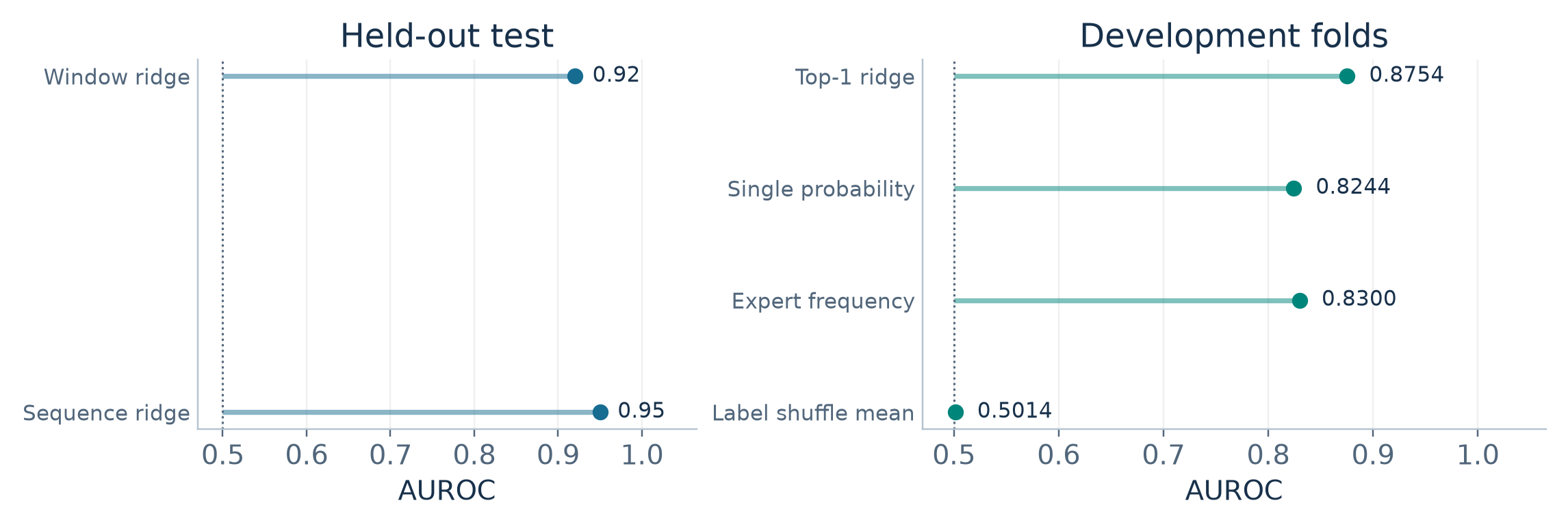
Figure 7. Redrawn from Section 4.1.2 and Table 2. Held-out results and development-fold controls are separated because their feature sets, data and scoring protocols differ.

For a scoring function $s(\cdot)$, AUROC estimates the probability that a positive example outranks a negative one, assigning half credit to ties. It is independent of a particular threshold. In Appendix Table 2, ridge on only the top-1 probability per depth reaches 0.8754 in development cross-validation, a single winning probability 0.8244 and frequency log-likelihood ratio 0.8300. Document-label permutations give mean 0.5014 and maximum 0.5231 across 99 runs. Those simpler readouts recover substantial signal, so confidence and ID frequencies both deserve consideration. The development scores cannot directly quantify how much performance the full router features add on the held-out split.

High AUROC under the sampled labels establishes that scores separate the two extremes of that classifier’s distribution. It does not settle whether the model would answer a harmful request, how well an alert threshold is calibrated, or whether the signal survives a change in language, domain or labeling convention. As an illustrative deployment calculation, at one percent prevalence with 90% true-positive rate and 5% false-positive rate, precision would be $0.009/(0.009+0.0495)\approx15.4\%$. Neither operating point is reported by LoL. A decision-grade evaluation would supply the actual threshold curve under target prevalence and measure first-detection time for partially observed documents.

Efficiency results and how to compare them

Math at 1B parameters

The math experiment uses 16 total applications with four prelude, eight core and four coda layers. LoL stores eight core experts. All runs use a mixture of Nemotron and OpenMath data, about 90 exaFLOPs, and the most compute-efficient model sees about 20B tokens. The paper matches parameter scale and compute and compares full, sliding and strided dense baselines. Appendix C.5 uses five shots except three on GSM8K to fit the 1,024-token context. Comparing loss across math and FineWeb would change the data distribution and the predictability of tokens.

Model (paper Table 5)	ARC-E	ARC-C	HellaSwag	PIQA	GSM8K
Vanilla full	40.8	28.2	31.4	56.6	29.7
Vanilla sliding	49.5	28.5	31.3	58.8	27.5
Vanilla strided	48.5	28.0	30.8	59.0	25.9
LoL	50.3	29.1	31.2	59.7	27.9
LoL untied router	50.1	30.0	31.4	57.1	27.7

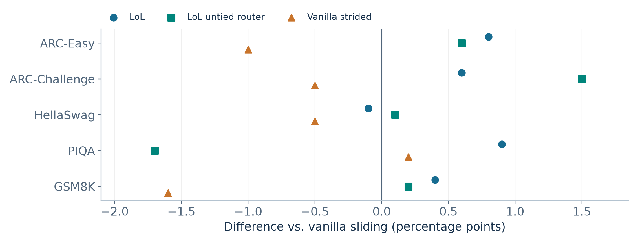
Figure 8. Redrawn as differences from vanilla sliding attention using paper Table 5. The paper reports per-model standard errors. The two-model differences shown here carry no error bars because the covariance between model scores is unavailable.

ARC-Easy illustrates why the baseline matters. LoL gains 9.5 percentage points over vanilla full attention but only 0.8 points over vanilla sliding attention and 1.8 points over vanilla strided attention. On GSM8K it trails vanilla full attention by 1.8 points and leads sliding attention by 0.4 points. These comparisons support competitiveness under the matched setup. They provide weaker evidence for a causal effect of dynamic layer order, since growth, attention pattern and routing differ between configurations. The standard errors in the table characterize benchmark estimates. They cannot substitute for repeated training runs with paired evaluation or show that two architectures are equivalent.

On one math model, paper Figure 4 shows that some experts are concentrated across neighboring depths and some span wider ranges. This provides descriptive evidence of specialization, and helps explain why swapping experts arbitrarily is a demanding intervention. It does not establish how the expert distribution would change with context length or instruction tuning. In Appendix Figure 20 the extended dense and untied-router comparisons finish at broadly similar training loss. A closer test of order would compare adaptive LoL to the same library running a learned, input-independent route under identical masks, FiLM, token exposure and growth schedule.

FineWeb and forced reuse

The Huginn comparison trains 360M-effective-scale models on 10B FineWeb tokens. At core depth 16, libraries of 2, 4 and 8 are matched to recurrent blocks of two layers looped eight times, four looped four times, and eight looped twice. The authors tune at least six learning rates, consider multiple schedules and tune Muon and AdamW separately for the comparisons. Figure 5 uses three seeds, reports their min/max as bars in the evaluation plot, and averages the training curves. LoL is competitive at these matched scales and has larger spread in final evaluation loss. The authors suggest router initialization changes which paths are explored, a hypothesis consistent with the diverse depth-expert matrices in Appendix Figure 21. Three seeds constrain that conclusion. They provide neither the distribution of final loss nor evidence that initial routes explain all the variation.

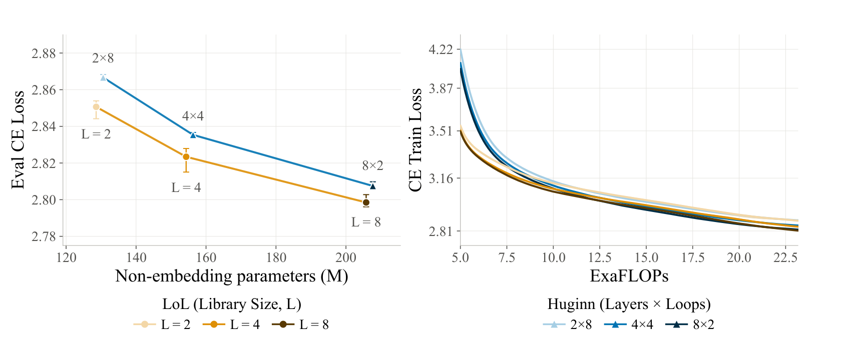
Figure 9. Cropped from paper Figure 5, p. 9. Left shows held-out cross-entropy versus non-embedding parameters with three-seed min/max. Right uses a training-FLOP axis and seed means.

Stored, effective and non-embedding parameter counts answer different questions. At fixed $D$ and width, reducing $L$ saves weight storage, while the same number of applications still consumes activations and compute. When a looped baseline shares blocks, reporting the “360M” effective scale alone can make two storage budgets look identical even when they differ. The matched-size points are more informative than a single headline comparison. The depth-expert matrix measures marginal use across windows. It cannot determine how many distinct experts a token actually sees. Equation (9) is a reference for a new path-level measurement, not a reinterpretation of Figure 21.

FineWeb and sparse MoE

The sparse comparison uses 24 library experts at 16 core depths against a conventional three-expert, top-two MoE. This matches a nominal 3:2 ratio. The authors increase MoE expert intermediate width to align active parameters, give LoL MoE prelude and coda blocks, and use strided attention at the same depths in the MoE baseline. Runs use approximately 17 exaFLOPs and the most efficient one sees around 10B tokens. Figure 6 reports a small terminal training cross-entropy advantage for MoE, about 2.75 versus 2.80 for LoL, despite LoL’s early advantage under growth. The 0.05 cross-entropy gap corresponds to an illustrative ratio of $\exp(0.05)\approx1.051$ in perplexity on the same tokenization and loss convention. It does not compare wall-clock, perplexity on a new dataset or performance on the 1B math tasks.

The nominal ratio has different meanings. In the MoE case two of three FFN experts are active per token at each layer. In LoL’s core one complete block runs per token per depth, and the ratio compares depth with the number of available blocks. Distinct experts per path can be fewer than 16. Even if two architectures have the same ratio of active parameter applications to storage, they can differ in cache reuse, communication and batch utilization. A marginal heatmap from one seed can hide concentrated use for a subset of requests. Appendix Figure 22 usefully shows different specialization profiles across seeds. A systems comparison needs both use per device and expert occupancy for each real scheduling step.

Limitations and reproducibility of the evidence

LoL’s natural-language pretraining uses 1,024-token contexts and relatively small models. The full outer stacks, moderate context and training metrics matter to interpreting generalization. Strided core attention cannot move every individual token representation arbitrarily far in one step. Global access through the coda, prelude and routing summaries has different capacity and cost. Larger models and more heterogeneous batches may trade weight storage for fragmented execution. The paper does not provide a decode or serving benchmark that measures this trade.

The released paper gives the architecture, mask and router, tokenizers, broad data construction, optimization setup and the ablation conditions. Appendix A specifies RoPE, RMSNorm, SwiGLU, bias-free attention, Muon alongside AdamW, document-blocked attention, and natural-language windows of 128 with stride 64. It uses GPT-NeoX tokenization for predominantly English FineWeb and OLMo3 for multilingual work. Synthetic first windows span the prompt and strategy field, and subsequent windows use 128/64 for sudoku and 64/32 for mazes. Those settings and the precise meaning of an input-dependent window are important when reproducing comparisons. I checked the equations and extracted figure and table values, and evaluated small arithmetic and dependency examples. The performance numbers in this review are the authors’ results.

For a matched experiment, log tokens seen, the growth trace, training FLOPs and the parameter counts before benchmarking. Save the exact split unit for documents, puzzles and maze seeds. Probe comparisons are sensitive to whether multiple windows from one document cross the split. Template extraction is sensitive to whether validation and test puzzles have shared grids and to missing or sparsely sampled cells. Capturing these quantities makes a disagreement diagnosable. Loss alone would not say whether a change came from routing, mask support, token count or a different intervention.

Critical analysis

Is the path a control variable or an algorithm?

The maze intervention demonstrates a meaningful control variable. The same output format and substantially different exploration orders make it harder to explain the result by syntax alone. But the strategy field is an explicit training-time channel into the router, and the learned representation is free to encode that condition in expert IDs, residual scales or the combination. The expert applied at one depth can depend on a depth-specific modulation, and later windows can reflect the already generated trace. It is possible for a stable early strategy cue to influence many later decisions without each named expert corresponding to a reusable search operation.

I would use a factorial intervention across gate and ID and a control that preserves counts while changing order. On each held-out grid, keep either the original gate, the forced gate, or a matched constant while changing the ID sequence. Compare the reported template to a permutation of its expert multiset that preserves per-expert counts. Keep output prefix, window partition and evaluation limits fixed. In a second experiment, replace one depth range at a time and include matched random perturbations of the same size. Report strategy, legal steps, final answer and their joint score. A coherent shift in strategy under count-preserving reordering, with legal trace and accuracy intact, would better support an ordering effect. A gate-only effect would instead point toward conditioning through amplitude. Unseen cyclic mazes, novel sizes and new label-to-strategy mappings would test generalization beyond the fitted generator.

A serving budget should measure reuse of weights and reuse of state

With cached autoregressive decoding, a reasonable reference implementation would keep a route and gate per live window and depth, plus the earlier window-mean sum and the current window’s running hidden-state sum. The running sum must be taken from the block input, as in Algorithm 1. For attention, tokens in the active window can append key-value pairs under the same expert. Once a core window closes, later windows at that depth access it through summaries, while prelude and coda maintain their full-context caches. Treating a reused expert as one cache across depths would be invalid in general because its inputs and FiLM differ. This is a consequence of the described architecture. The paper does not present this cache as a measured result.

Even a latency budget with equal active FLOPs can reverse with smaller or more scattered expert groups. As an illustrative cold-weight accounting, let $B$ be the number of active windows at a decode step and $U_b$ their distinct selected experts at one routed depth. Ignoring reuse across kernel calls and assuming one load per used expert, a cold-read weight budget at that step is approximately $U_b$ times bytes per expert. When all windows choose the same block, $U_b=1$. When eight windows choose eight experts, $U_b=8$. Under ideal uniform independent routing with $L=24$ and $B=8$, equation (9) with $B$ draws gives about 6.93. Real kernels can reuse weights from cache or combine work across requests, so the value is an accounting illustration. It explains why evaluating resident weights, HBM traffic, expert dispatch, occupancy and p95 per-token latency separately is more informative than reporting active FLOPs. Burst tests should vary whether requests hit window boundaries together and whether a prefill is concurrent with decode.

Is dynamic order worth its optimization burden?

The paper’s strongest efficiency evidence is that this architecture can learn under very different storage regimes. A decisive comparison for adopting it would train a fixed shared-library route and an adaptive route with the same growth schedule, router overhead budget, mask and modulation. A fixed route could be optimized offline or based on the most common path. A second baseline could choose once at a boundary and reuse its path for the entire next segment. This would trade responsiveness for fewer routing decisions and larger expert batches. Sweep $L$, $D$, $W$ and $S$ under matched measured time as well as reported FLOPs, and plot quality against both parameter bytes and p95 decode time. Include route concentration and marginal expert load so that a small gain can be attributed to input adaptivity rather than to added parameter capacity or a more favorable training schedule.

There is a second opportunity in the pooling rule. Summarizing all completed windows gives older windows influence indefinitely but dilutes a recent event as $1/k$. Adding a new mean $\mu_k$ changes the cumulative router input by $(\mu_k-r_k)/(k+1)$. At long context, a decisive token in a full new window first receives a $1/W$ mean coefficient and then a $1/(k+1)$ prefix coefficient. A learned decay or separate summary for the most recently completed window preserves causality and may improve responsiveness. It also risks overreacting to noise. A boundary-sensitive benchmark can insert a decisive cue at different positions and measure when and how strongly the route changes while controlling the token count and answer. That test would connect the current evidence about language and strategy to the actual time at which the architecture can use new information.

Conclusion

Library of Layers makes the order and reuse of whole transformer blocks depend on the input while maintaining a fixed number of core applications. Its most instructive mechanism is the combination of same-expert causal attention within a window, prefix-only selection and shifting boundaries across depth. The results support a feasible architecture and a strategy-control mechanism on deliberately constructed tasks. The next evidence I would look for is a controlled comparison that isolates dynamic order, plus a decoding benchmark that charges the actual cost of moving weights and maintaining per-depth state.

Technical references

• Rahmani et al., Library of Layers, arXiv 2611.03526v1. Sections 3–5, Algorithm 1, and Appendices A–C supply the architecture and results discussed here. Paper PDF · Authors’ project resource
• Geiping et al., Scaling up Test-Time Compute with Latent Reasoning. Background for the Huginn-style depth recurrence baseline. Paper
• Wang et al., Auxiliary-Loss-Free Load Balancing Strategy for Mixture-of-Experts. Background for the selection bias separated from residual weighting. Paper
• Pérez et al., FiLM: Visual Reasoning with a General Conditioning Layer. Background for depth-conditioned feature scales and shifts. Paper