Low-Rank Key Value Attention | What a shared cache can preserve

Review date: 2026-11-07
Author: Zhongzhu Zhou
Paper reviewed: Low-Rank Key Value Attention
Paper authors: James O’Neill, Robert Clancy, Mariia Matskevichus, Fergal Reid
arXiv: 2601.11471, version v3, 2026-04-07

1. The unit of compression is the head residual

A serving system can run out of cache capacity even when the model weights fit comfortably. Each generated token adds key and value coordinates at every layer, and every live sequence keeps its own history. The authors of LRKV address this cost in the model architecture. They train every head to read a shared dense key and value projection, then give each head a small private correction. The cache stores one copy of the shared features and only the low-dimensional coordinates of each correction.

I find the choice of what to share more interesting than the headline memory percentage. Grouped-query attention shares entire projections within each group. LRKV instead shares a baseline across the layer, while the residual rank sets a budget for head-specific changes. A shared key can capture a feature that all queries consult. A private correction lets one head refine the feature map used to score a token. Values follow the same construction with separate parameters.

The authors compare five attention families across four nominal sizes from 128M to 6.3B. The table of final losses favors LRKV at all four scales under the selected configurations. The paper also reports a higher mean across five downstream benchmarks after supervised midtraining. Its approximately half-size cache compares against multi-head attention, while selected GQA and MLA configurations use still less cache. I distinguish those quality and storage comparisons from the unmeasured wall-clock behavior of the proposed factored decode path.

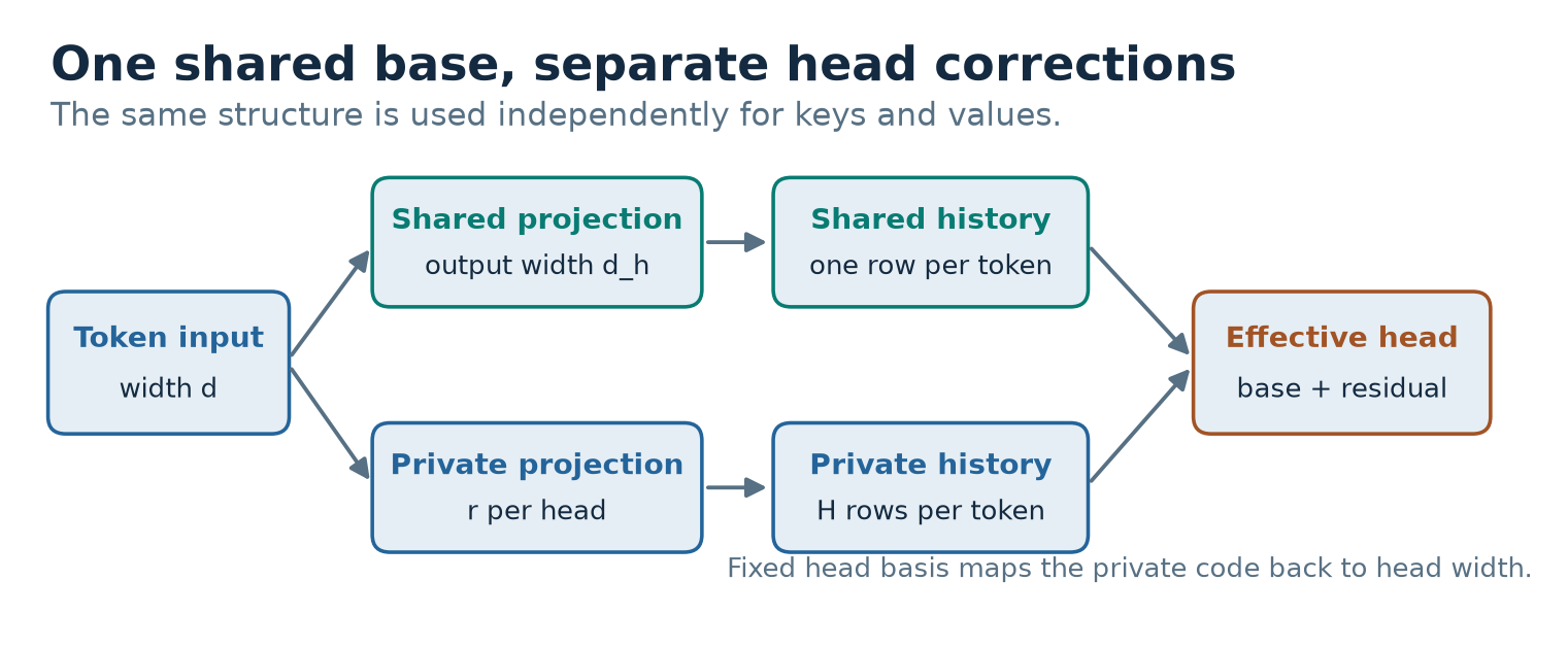
Figure 1. Original schematic based on paper Fig. 1 and Eqs. 2–5. Each row of the history retains shared coordinates and two sets of private latents per head. The small reconstruction matrices belong to the layer weights.

2. Prerequisites

Attention as routing and retrieval

Let $X$ have $T$ token rows and $d$ columns. There are $H$ query heads with $d_h$ coordinates each. The key and value matrices of head $h$ each have shape $T\times d_h$. A query row $q_h$ uses dot products with key rows to choose how much value content to read. Scaling by the square root of head width controls the typical magnitude of the raw dot products. The causal mask supplies negative infinity for positions outside the visible history.

$$\begin{aligned} s_{h,j}&=\frac{q_h k_{h,j}^{\top}}{\sqrt{d_h}}+m_j,\\ a_{h,j}&=\frac{\exp(s_{h,j})}{\sum_i\exp(s_{h,i})},\\ o_h&=\sum_j a_{h,j}v_{h,j}. \end{aligned}$$

The score and value roles matter when we move operations around. Softmax couples all visible tokens and is nonlinear. The weighted sum of values is linear once the weights are fixed. A valid factorization adds shared and private logits before softmax, then adds shared and private value contributions under the same weights. Two independently normalized attention calls generally yield a different result. For example, logits $(2,0)$ and $(0,2)$ give uniform weights after addition, while either branch alone concentrates its weight on one token.

Where the bytes go

Autoregressive decoding can retain the keys and values for previous tokens because a causal model never updates their states in response to later tokens. Prefill initially constructs these features for the input. Each decode step writes one new row and reads the relevant history. The query usually lives only for that step. For $N$ layers, batch $B$, equal-length histories, and $b$ bytes per stored scalar, the dense cache payload is

$$M_{\mathrm{MHA}}=2bNBT H d_h.$$

The first factor of two counts key and value. With uneven lengths, replace $BT$ by the sum of the live sequence lengths before accounting for allocator padding. Training has a different memory budget. Activations for backpropagation, optimizer state, model weights, and attention workspaces can dominate. Section 3 describes materialized K/V during training, so the compressed inference cache gives no direct factor of two for training memory.

Rank and the scope of the constraint

A product of a $d\times r$ matrix and an $r\times d_h$ matrix maps through an intermediate space of at most $r$ dimensions. The image of the product therefore has rank at most $r$. If I add a dense matrix of the same output shape, the sum can have full column rank. LRKV constrains the difference between a head and the common projection. The distinction explains how a head can still emit a $d_h$-wide key even when its private code has only $r$ coordinates.

For a fixed common matrix, truncated SVD of a target head’s residual gives the best rank-$r$ approximation in the Frobenius norm. The squared error is the sum of squared discarded singular values. The trained model in this paper solves a different optimization problem. It learns the common matrix, private factors, queries and the rest of the model under language-model loss. Frobenius error gives a useful geometric comparison. Loss depends on the data distribution, the scaling of the logits, values and downstream computation.

3. Training and the cache representation

From a weight factorization to token coordinates

Write $W_S$ for the common projection of either key or value. With $U_h$ of shape $d\times r$ and $B_h$ of shape $d_h\times r$, paper Eqs. 2–5 are an application of distributivity and associativity. Superscripts $K$ and $V$ select independent copies of the construction.

$$\begin{aligned} W_h &= W_S + U_h B_h^\top,\\ X W_h &= XW_S + X(U_h B_h^\top)\\ &= XW_S + (XU_h) B_h^\top\\ &= S+R_h B_h^\top. \end{aligned}$$

The common row $xW_S$ has $d_h$ entries. The private row $xU_h$ has $r$. Both are computed from the same token activation and preserve its time index. In inference a token’s private row is stored as soon as it is produced, avoiding the need to keep the original hidden activation around. That is a change in cache layout for a model trained with these factors. It differs from taking an arbitrary trained MHA checkpoint and truncating its weights.

At zero private width the design implements MQA-style K/V sharing within a layer. At full width the residual can represent any matrix of that shape, and the architecture can express arbitrary independent projections. Its factored storage at that endpoint exceeds MHA because it still pays for the common features. The authors train the dense base jointly with small randomly initialized residual factors. Zeroing both factors would make both residual gradients vanish initially.

To see the optimization paths, let $G_h$ be the loss derivative with respect to the effective projection $W_h$. Expand the differential into a base variation and two residual variations. Matching coefficients in the Frobenius inner product yields

$$\begin{aligned} dW_h &= dW_S+(dU_h)B_h^\top+U_h(dB_h)^\top,\\ \nabla_{W_S}\mathcal L &=\sum_h G_h,\\ \nabla_{U_h}\mathcal L &=G_h B_h,\qquad \nabla_{B_h}\mathcal L=G_h^\top U_h . \end{aligned}$$

The base receives gradients from every head. The factors absorb private changes through a bilinear update. A single common projection costs less cache than one per group, but leaves more work to the private path if the layer contains several different head families. A grouped shared base could trade an extra set of common coordinates for smaller private widths. That trade needs separate training and evaluation.

Algorithm 1. Construct the factored cache

This pseudocode follows Section 3 in its linear pre-position form. The same construction appends the new token after prefill. Prefill attention during training can materialize each effective head tensor.

01  Receive layer activations X for the new token rows.
02  Project S_K = X W_S_K and S_V = X W_S_V once.
03  Append S_K and S_V to the shared histories.
04  For each head h, form R_K[h] = X U_K[h].
05  Form R_V[h] = X U_V[h] for that same head.
06  Append both private blocks at the matching token indices.
07  Keep the head matrices B_K[h], B_V[h] with the weights.
08  Keep sequence boundaries and positions with the cache.

Associative decode

For a single query, expand the transpose of the factored key. Moving $B_h^K$ to the query side changes the order of contraction while keeping the resulting score vector of length $T$.

$$\begin{aligned} q_h K_h^\top &=q_h(S_K+R_h^K(B_h^K)^\top)^\top\\ &=q_h S_K^\top + q_h B_h^K(R_h^K)^\top\\ &=q_h S_K^\top + (q_h B_h^K)(R_h^K)^\top . \end{aligned}$$

The query-side projection costs one small multiplication per head per step. The private dot products then scan a narrower history. The denominator remains $\sqrt{d_h}$ because the summed score represents the original full-width dot product. Scaling one branch by $\sqrt r$ would change its relative influence.

After the single softmax, value aggregation follows the other contraction order. Compute a full-width common weighted sum and a rank-width private weighted sum. Apply $B_h^V$ to the latter once per head and query.

$$\begin{aligned} a_h V_h &= a_h(S_V+R_h^V(B_h^V)^\top)\\ &= a_h S_V+(a_h R_h^V)(B_h^V)^\top . \end{aligned}$$

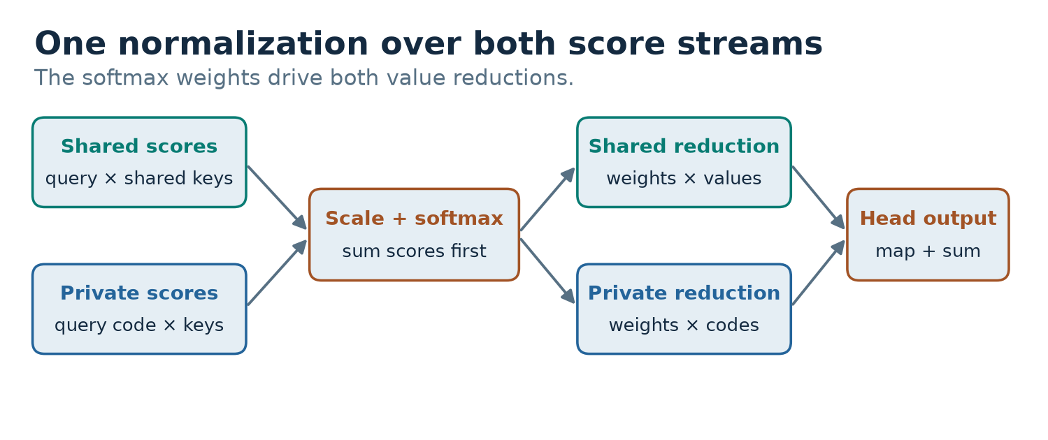
Figure 2. Original dataflow from paper Eqs. 6–7. Both score streams enter the same softmax. The resulting token weights drive both value streams.

Algorithm 2. Decode against the factored history

The algorithm describes exact real-arithmetic equivalence to materializing the same factored linear projections. Floating-point reduction order can change the last bits. The treatment of RoPE and post-projection normalization requires additional work discussed below.

01  For each head h, project q from the current token.
02  Project p = q B_K[h] once.
03  For each visible row j, sum two score terms.
04  Use dot(q, S_K[j]) plus dot(p, R_K[h,j]).
05  Scale the sum by sqrt(head width) and mask it.
06  Normalize the summed scores over visible rows.
07  Reduce S_V and R_V[h] using those same weights.
08  Map the private reduction through transpose(B_V[h]).
09  Add both reductions, concatenate heads and project out.

A fused version can maintain an online softmax. In each history tile, compute the sum of the score terms before updating the running maximum. Carry a shared-value accumulator of width $d_h$ and a private accumulator of width $r$ per query head. If a tile increases the running maximum, rescale both accumulated numerators and the denominator by the same exponential factor. After the last tile, divide both accumulators by the denominator and apply the value projection to the private part. The larger accumulation state can raise register pressure. It creates a trade-off between head grouping for cache reuse and occupancy.

For a small hand calculation, take $q=(2,1)$, the shared key $(1,3)$, a private latent $4$ and reconstruction column $(1,-1)^\top$. The materialized key is $(5,-1)$, so the dot product is $9$. The common dot product is $5$ and the query projected into the private coordinate is $1$, giving $5+4=9$. If the value weights are $(1/4,3/4)$ and private value coordinates are $(2,6)$, the weighted private coordinate is $5$. With column $(1,-1)^\top$, it contributes $(5,-5)$ to the shared output. These are illustrative calculations.

4. Accounting for cache, parameters and decode cost

A cache budget gives a rank ceiling

The two shared tensors hold $2Td_h$ scalars per layer and sequence. The $H$ private pairs hold $2THr$. Dividing by the MHA payload cancels precision, length and layer count under equal assumptions. Set a target fraction $c$ and solve for the allowable integer rank.

$$\begin{aligned} M_{\mathrm{LRKV}} &= 2bNBT(d_h+Hr),\\ \frac{M_{\mathrm{LRKV}}}{M_{\mathrm{MHA}}} &= \frac{1}{H}+\frac{r}{d_h},\\ r &\le \left\lfloor d_h(c-1/H)\right\rfloor . \end{aligned}$$

For $H=18$, $d_h=128$ and $c=0.5$, a rank of at most $56$ fits the algebraic payload budget. Table 7’s $r=55$ gives $48.52\%$. An alignment-constrained kernel might choose $48$ or pad a rank of $55$ to a physical width of $64$. Padding changes the actual layout and moves the latter to $55.56\%$. The formula also gives a quick comparison with GQA. Six equal groups at 18 heads store a third of the dense cache. To fit that payload with LRKV would require rank at most $35$, a separate quality operating point.

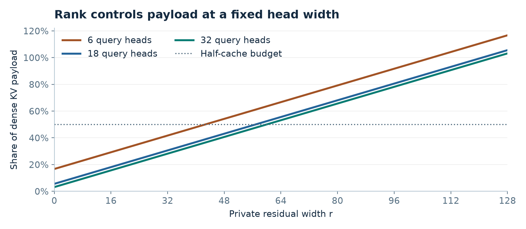
Figure 3. Original calculation from paper Eq. 9. The slope is fixed by head width. Increasing the number of heads only shrinks the common-base intercept.

Consider Table 5’s 18-layer, 18-head, 2.5B layout and BF16 with 2,048 history tokens. Dense storage is $339{,}738{,}624$ bytes, or 324 MiB per sequence. The ideal rank-55 layout gives 157.21875 MiB. This example uses the stated layer count and excludes padding and position-dependent auxiliary data. At 8,192 tokens, the two numbers scale to 1,296 and 628.875 MiB. In a serving system these bytes compete with paged allocation slack, workspace and the model weights. A ratio near one half for payload can raise capacity substantially when the cache dominates the memory budget.

Weight count and the two decode regimes

For keys and values together, the common projections contribute $2dd_h$ weights. The two private factors each add $r(d+d_h)$ weights per head. With other model components fixed, the resulting ratio relative to MHA’s K/V projection parameters is

$$\frac{P_{\mathrm{LRKV}}}{P_{\mathrm{MHA}}} = \frac{1}{H} + \frac{r}{d_h}\left(1+\frac{d_h}{d}\right).$$

At $d=2304$ and $r=55$, this is about $50.9\%$ for the K/V weights. The relative difference over the whole model is smaller because the feed-forward layers, embeddings, queries and output projections are outside this count. Appendix D names sizes using the MHA reference architecture. Matching nominal size holds many dimensions fixed while allowing parameter counts to differ. That is a reasonable architecture swap comparison and a separate question from parameter-matched scaling.

Ignoring softmax and other common operations, per head the two history contractions cost roughly $2Td_h$ multiply-accumulates in MHA. Factored decode adds $2Tr+2rd_h$. The first term comes from the private score and value scans. The second comes from the two per-step basis transforms. The arithmetic ratio in this simplified model is

$$\frac{C_{\mathrm{LRKV}}}{C_{\mathrm{MHA}}} \approx 1+\frac{r}{d_h}+\frac{r}{T}.$$

A bandwidth-limited decoder could benefit if it reuses the same common tile across many heads. If it fetches the entire common block afresh for every head, that block alone can require as many reads as MHA. A compute-limited decoder pays for both scans and the transforms. At short history lengths, launch overhead and basis loads can matter more than the saved payload. The larger temporary accumulators and the memory traffic for per-token projections can also shift the crossover. The paper reports cache accounting and loss curves. Its reported data do not locate the hardware crossover.

Tensor parallelism can replicate the shared block

The single-device cache formula counts one common block per layer. Suppose $P$ tensor-parallel shards split the query heads evenly and each shard needs its own local copy of the common features. Across all shards, one history token then occupies $2b(Pd_h+Hr)$ bytes. Dividing by dense MHA under the same head partition yields

$$c_{\mathrm{replicated}}=\frac{P}{H}+\frac{r}{d_h}.$$

For an illustrative deployment with 32 heads, four shards and rank 54 at head width 128, the ratio moves from about 45.3% to 54.7%. Both figures are arithmetic payload estimates. Each shard can reuse its common cache locally, while the aggregate common footprint rises. A single physical copy would need inter-shard reads, broadcasts or a different attention partition. Key and value features may also be recomputed locally on append if the input activation is already replicated. The best placement depends on how fast the device interconnect is relative to local memory and how much of each tile is reused. GQA and MLA have their own head or latent replication policies, so their unsharded cache percentages also need a specified layout.

Capacity and latency have different break-even points

For an illustrative lower-bound model, let $M$ be dense cache bytes actually read by a step, $F$ its arithmetic, $\beta$ effective bandwidth and $\phi$ effective compute throughput. Ignoring other work, a roofline estimate takes the larger of $M/\beta$ and $F/\phi$. With perfectly reused common tiles and no padding, the factored path scales the first term by its payload ratio $c$ and the second by its arithmetic ratio $a$. If dense MHA is bandwidth bound, a necessary condition for this simplified factored path to beat the dense bound is $aF/\phi < M/\beta$. This condition can fail even when $c$ is well below one. In a long-history example with $r=55$, $d_h=128$, the arithmetic multiplier approaches 1.43. If dense attention is already near the balance point, the new computation can erase much of the expected gain. The estimate excludes projection loads, occupancy changes and kernel launches. I use it to select test points on both sides of the bandwidth-to-compute transition.

5. Experiments and what the comparisons establish

Four scales under the same training recipe

The authors pretrain decoder-only models on FineWeb-Edu using mixed-precision BF16 on one eight-H200 node. The main comparison uses 2,048-token sequences, with 100B tokens for the 128M model and 50B for the larger models. Appendix D gives 32,768 tokens per effective batch and a Muon plus AdamW optimizer split. Each attention family keeps the rest of the nominal architecture fixed. The experiment therefore asks what happens when attention is swapped under this recipe.

Cross-entropy is the average negative log probability of the observed token. Bits per byte rescales total negative log likelihood by the number of text bytes and by $\ln 2$. A token average and a byte average can produce different magnitudes even when both are computed correctly.

$$\mathrm{CE}=\frac{-\sum_i\ln p(x_i\mid x_{<i})}{n_{\mathrm{tok}}}, \qquad \mathrm{BPB}=\frac{n_{\mathrm{tok}}\mathrm{CE}}{n_{\mathrm{byte}}\ln 2}.$$

The following values are the final held-out cross-entropies from paper Table 1. Boldface identifies the lowest displayed value per scale. The paper’s main prose highlights 128M and 2.5B, while the final tabulated values favor LRKV at the other two scales as well.

Attention	128M	1.2B	2.5B	6.3B
MHA	2.903	2.530	2.389	2.319
GQA	2.918	2.536	2.397	2.354
MQA	2.929	2.573	2.408	2.304
MLA	2.901	2.564	2.392	2.377
LRKV	2.893	2.509	2.376	2.288

At 2.5B, LRKV’s 0.719 BPB compares with 0.723 for MHA and 0.724 for MLA. The absolute CE difference from MHA is 0.013, about 0.54% relative to MHA. At 6.3B the nearest baseline by CE is MQA, with a difference of 0.016. A small, directionally consistent loss improvement is useful evidence under the selected conditions. A single displayed result per setting leaves the size of seed and recipe effects unresolved.

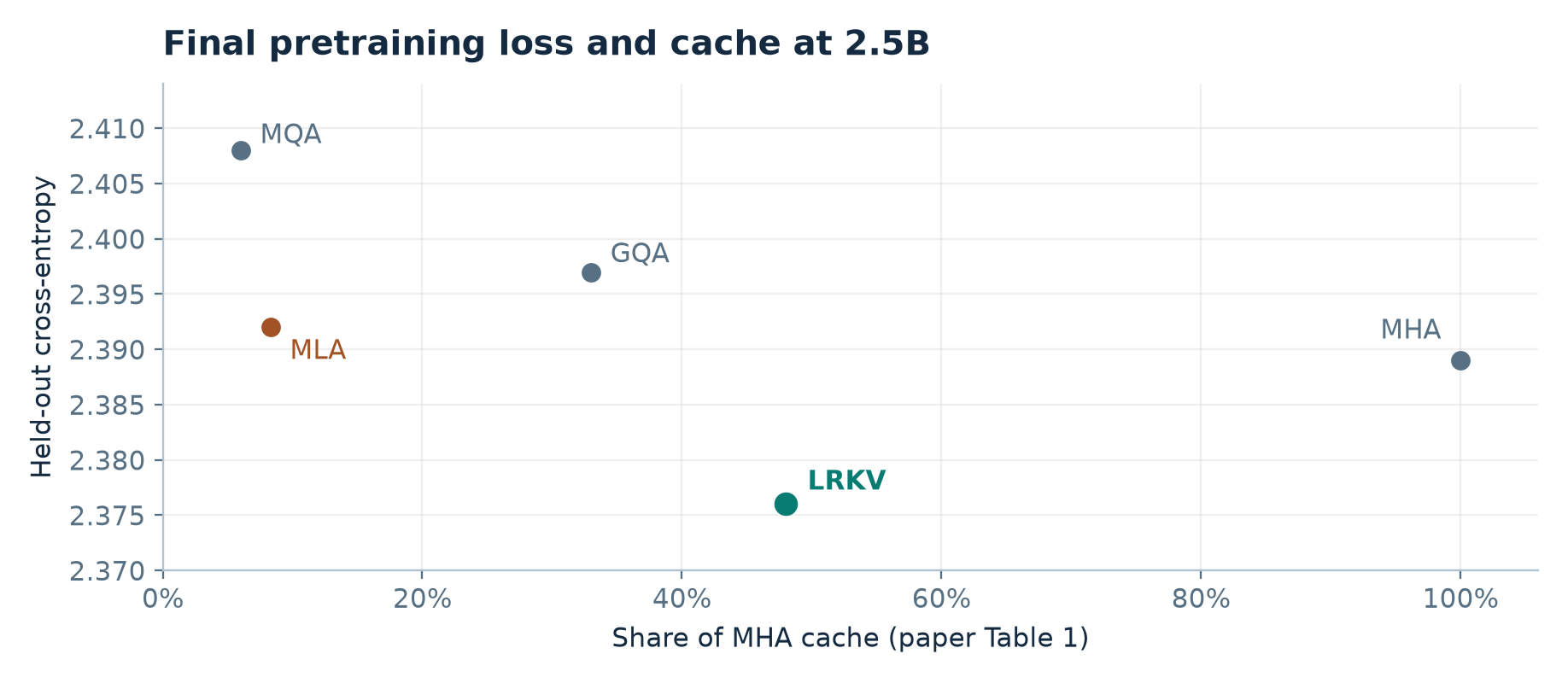
Figure 4. Redrawn from paper Table 1. Lower and farther left are favorable. LRKV improves on the dense reference on both axes here. MLA, GQA and MQA remain distinct choices when a smaller cache is the primary constraint.

Steps to reach a loss threshold

Paper Fig. 3 uses each baseline’s final validation loss as a separate target for LRKV. The targets are reached with reported savings of 29.7% against MQA, 21.4% against MLA, 24.5% against GQA, and 18.7% against MHA. The arithmetic mean of those displayed percentages is 23.575%. An easier target can be crossed sooner, so this is a set of baseline-dependent comparisons. Figure 2 adds an estimated compute axis. The paper’s footnote qualifies the quoted saving as sample efficiency and notes that training materializes full K/V.

In a repeat run I would freeze the targets before inspecting the curves, define the interpolation rule between evaluation points, and report steps, consumed tokens and actual accelerator-hours separately. Different optimizer dynamics or fused training kernels can shift the relationship between steps and elapsed time. The 18.7% MHA-target number is an interpretable comparison even if the average across four different targets is left aside.

Rank changes the frontier

The 128M sweep in Table 8 varies rank while holding its training token budget at 100B. Rank 8 gives CE 2.908, slightly above MHA’s 2.903. Rank 32 gives 2.896 at 41.7% of dense cache. Rank 64 gives 2.888 at 66.7%, and rank 128 gives 2.877 at 116.7%. The direction is monotonic across the reported ranks. The best loss in the sweep uses more cache than dense attention.

The paper also includes a latent-width sweep for MLA. Table 8 lists CE 2.894 and BPB 0.875 for MLA with a latent width of 384, at 25% cache under the table’s payload formula. Rank-64 LRKV reaches 2.888 CE and the same displayed BPB, at 66.7%. The result motivates two comparisons. One can compare the best quality at a fixed mathematical payload. One can also compare wall-clock decoding at matched quality with well-optimized kernels. The second is needed to adjudicate the reconstruction argument. The first does not establish that every LRKV point dominates every MLA point.

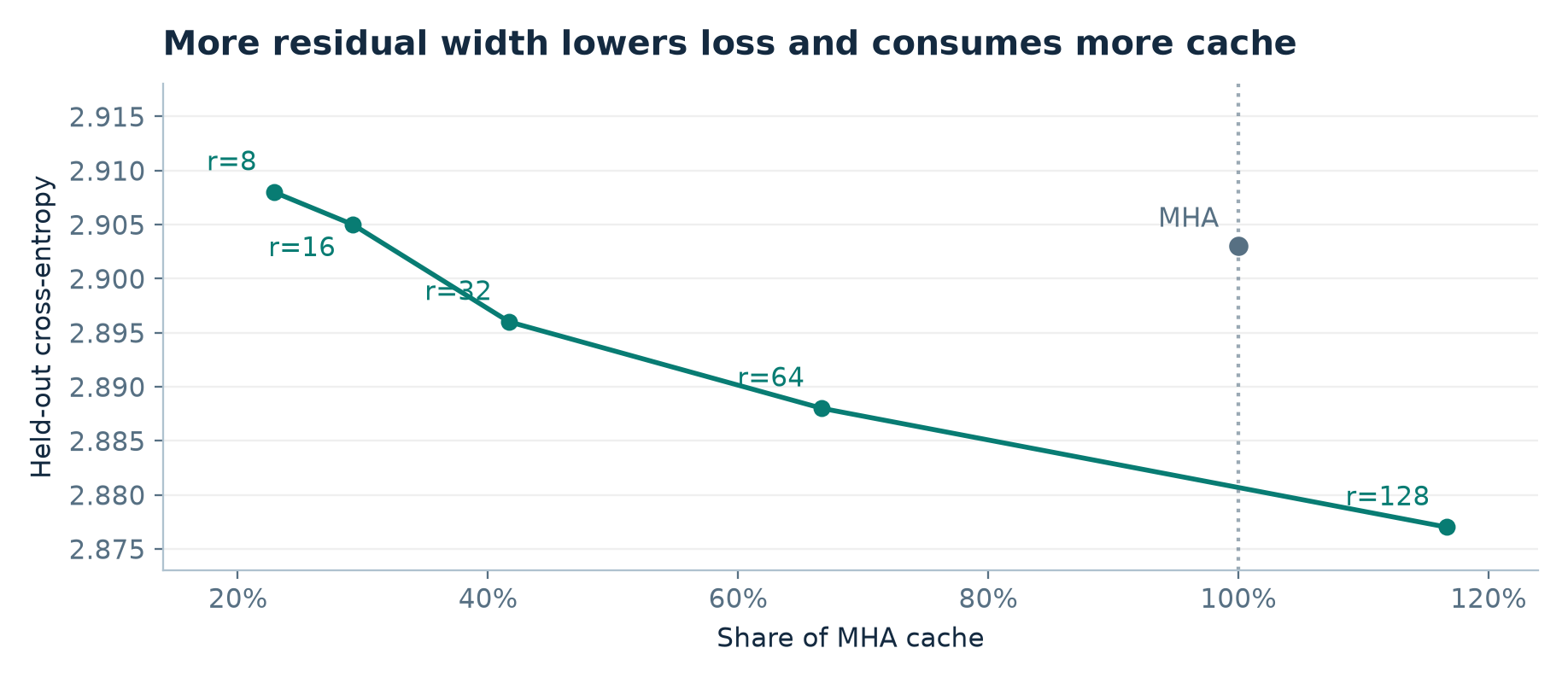
Figure 5. Redrawn from paper Table 8. Points show the five residual widths and the dense baseline. Connecting LRKV points is a guide to the eye. The sweep demonstrates the price of rank, including the point where the architecture spends more cache than MHA.

Midtraining and the long-context check

Appendix D describes one supervised pass over about 568K examples, mainly SmolTalk plus MMLU auxiliary training data and GSM8K. Paper Table 2 gives the best displayed five-task aggregate to LRKV at the three evaluated scales. At 2.5B it reports 37.9% versus 35.3% for MHA and 36.9% for MLA. The aggregate conceals movement in opposite directions. ARC-Challenge rises from 47.1 to 53.8, while HumanEval falls from 13.4 to 11.7. At 128M, GSM8K is 0.3 for LRKV versus 1.0 for MHA. At 6.3B, LRKV’s reported combined 40.2 leads MHA’s 38.8, while HumanEval again favors MHA.

Appendix E reports a relationship between BPB and downstream mean across the five architectures. With five points and a shared training recipe, this is a descriptive association. Architecture can move both outcomes, and midtraining adds another mechanism for differences to emerge. The gap in final BPB cannot by itself be assigned causal responsibility for the downstream gap. Task-level sample counts, prompt settings, confidence intervals and run variation would make the aggregate easier to interpret.

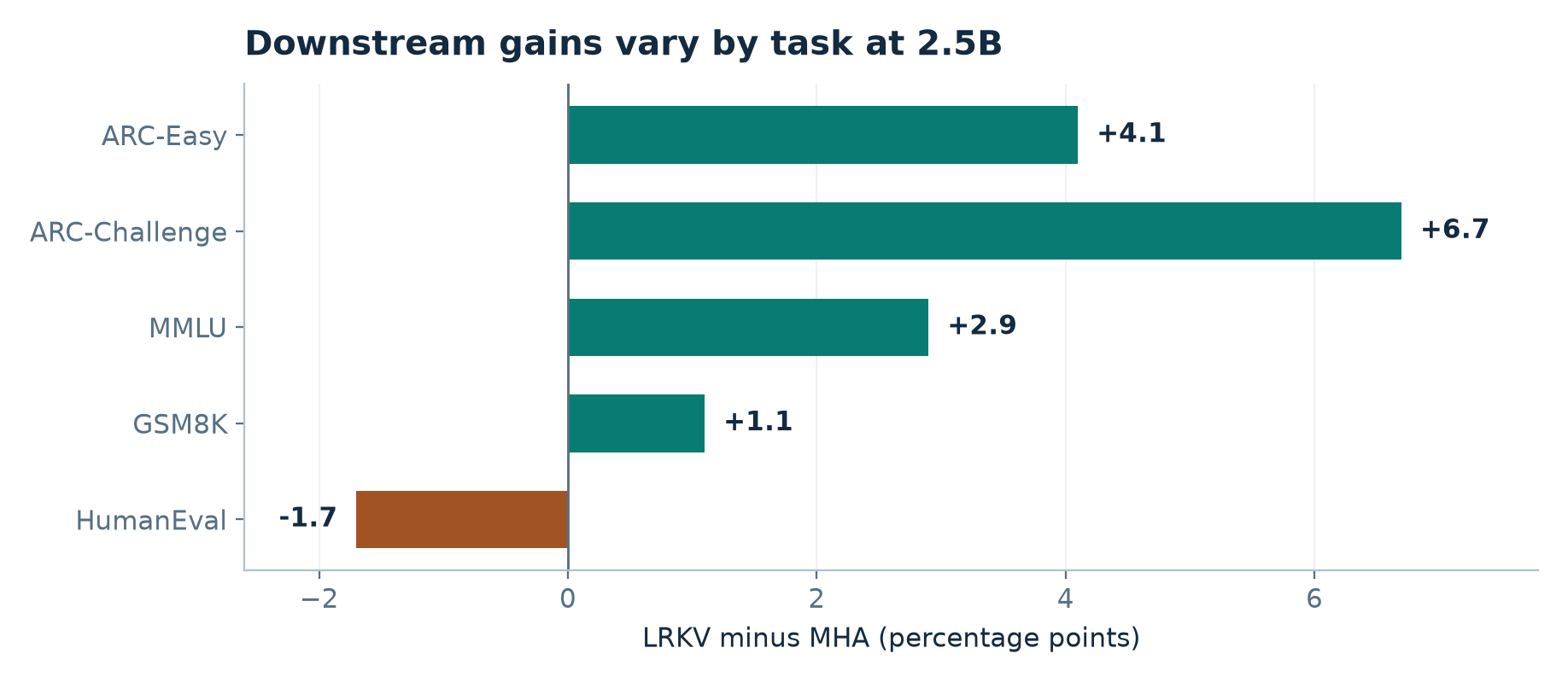
Figure 6. Percentage-point changes recomputed from paper Table 2, LRKV minus MHA at 2.5B. Positive values favor LRKV. The HumanEval result moves against the aggregate trend.

A separate 512M comparison extends training to 8,192-token sequences for 50B tokens, keeping the nominal tokens per batch fixed. Table 9 reports CE 2.665 for LRKV against 2.740 for MHA. Dividing the 0.075 absolute difference by 2.740 yields a 2.74% relative decrease. LRKV’s Table 7 rank of 51 at 12 heads yields roughly 48.18% cache under Eq. 9. The experiment supports the architecture at this trained context length. Document-average loss can hide retrieval failures at particular depths or positions. Retrieval of rare spans, cross-document interference and performance beyond the training window remain separate questions.

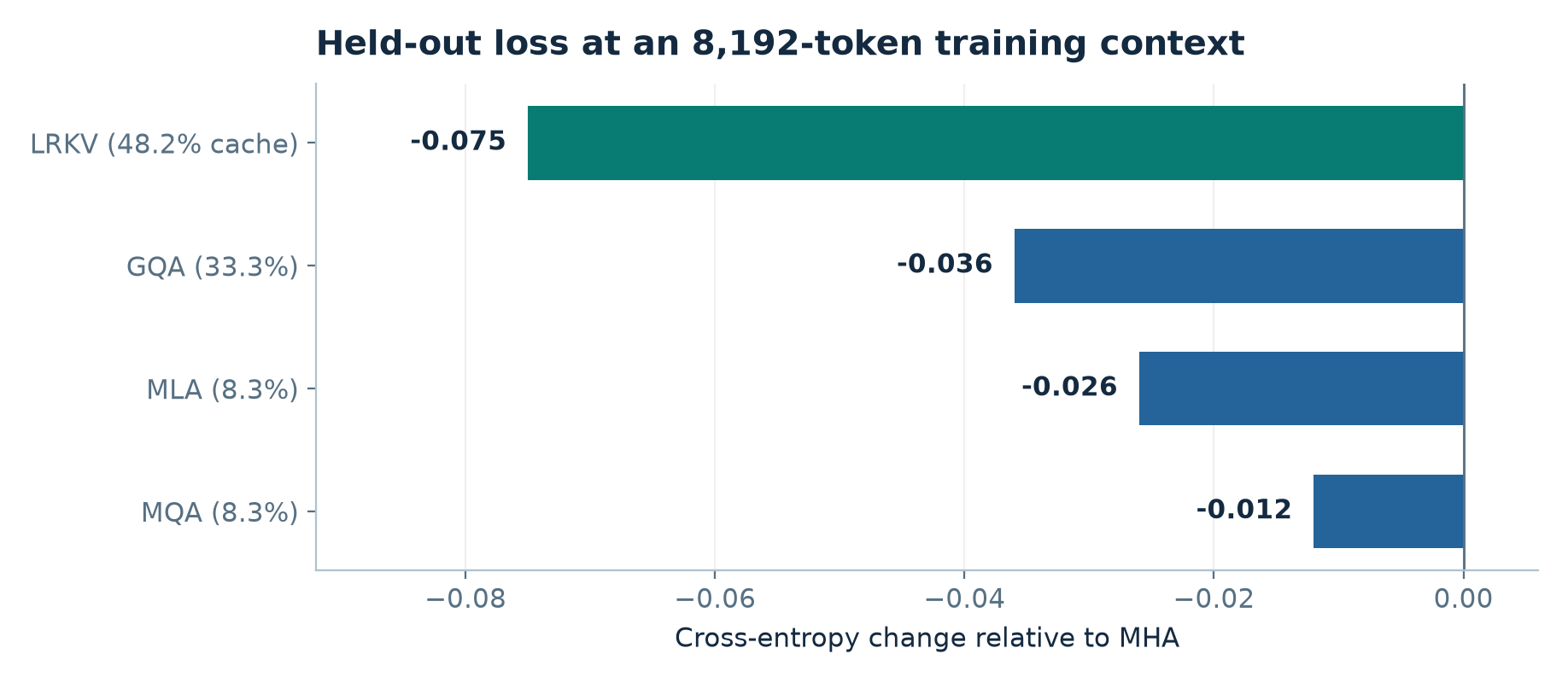
Figure 7. Redrawn from paper Table 9. The chart shows absolute CE changes relative to MHA under the 8,192-token training setup. Cache percentages are the paper’s payload estimates.

6. How the paper measures head diversity

A coordinate-invariant object for linear logits

For two input rows $x$ and $y$, the unnormalized linear score is $xA_h y^\top$ with $A_h=W_h^Q(W_h^K)^\top$. Rotating both head coordinates by the same orthogonal $R$ leaves the score unchanged because $RR^\top=I$. For the linear case, the same reasoning extends to any invertible query transform with the inverse transpose on keys. Comparing raw key weights can thus distinguish two equivalent logit maps. Comparing $A_h$ removes this ambiguity for the linear model.

$$\begin{aligned} A'_h &= (W_h^Q R)(W_h^K R)^\top\\ &= W_h^Q RR^\top(W_h^K)^\top=A_h . \end{aligned}$$

To compare two heads, insert their factorizations into the Frobenius inner product and cyclically rotate the trace. The resulting calculation uses small head-width matrices rather than explicitly allocating the $d\times d$ score maps.

$$\begin{aligned} \langle A_i,A_j\rangle_F &= \operatorname{tr}(W_i^K (W_i^Q)^\top W_j^Q (W_j^K)^\top)\\ &= \operatorname{tr}\big((W_j^K)^\top W_i^K (W_i^Q)^\top W_j^Q\big). \end{aligned}$$

The paper normalizes by individual Frobenius norms for its similarity scores. This treats head-map direction as the object of study. If $F$ has one row per flattened, normalized map, $G=FF^\top$ is the cosine Gram matrix. Multiplying by $J=I-\mathbf 1\mathbf 1^\top/H$ subtracts the sample mean from each row. Thus centering the maps and taking their Gram matrix is equivalent to a small matrix operation.

$$\begin{aligned} F_c&=JF,\qquad G_c=F_cF_c^\top=JGJ,\\ p_i&=\lambda_i/\textstyle\sum_j\lambda_j,\qquad r_{\mathrm{eff}}=\exp\big(-\textstyle\sum_{i:p_i>0}p_i\ln p_i\big). \end{aligned}$$

Equal positive eigenvalues yield an effective rank equal to their count. One dominant eigenvalue lowers it. The centered matrix has at least one null direction because $J\mathbf 1=0$. If all maps are identical, every centered eigenvalue vanishes and the normalization is undefined. A diagnostic should handle that case explicitly. If the denominator for percentage effective rank is $H$, as Table 3 states, the centered ceiling is $(H-1)/H$. The ceiling is 83.33% at six heads and 94.44% at eighteen heads. A 93.5% centered score is close to the ceiling of its construction.

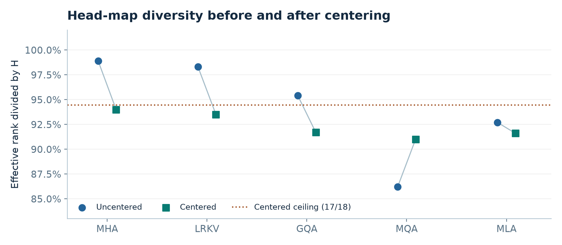
Figure 8. Redrawn from paper Table 3 at 2.5B. The dotted line shows the centered ceiling when percentages divide by 18. Uncentered scores can exceed that line. The chart compares map spectra at a checkpoint and does not measure task-level specialization.

The centered LRKV and MHA values at 2.5B are 93.5% and 94.0%. MQA’s 91.0% centered score is above its 86.2% uncentered score. Centering removes a common direction that can dominate the raw spectrum. If all keys are shared, distinct query projections can still generate different score operators. The observation is consistent with this compensation story. An intervention on the query projections would be needed to show that training used it to preserve task performance. Appendix C’s spectra, similarity heatmaps and cumulative variance plots are complementary descriptions of the same parameter-space geometry.

Figure 9 of the paper is captioned as centered effective rank for six heads, yet several plotted values appear above five. Under the centered Gram construction described in Appendix C, five is the maximum raw effective rank. I use the labeled aggregate cells in Table 3 for the chart here and would request the raw spectra and the denominator used in each panel before drawing a layer-by-layer conclusion.

7. Limitations acknowledged by the paper

Appendix H bounds the reported results to decoder-only language models, a particular optimizer and data recipe, sizes up to 6.3B, and the hardware used for evaluation. Appendix C adds that its diversity analysis looks at final checkpoints and measures potential diversity in weights. Neither the rate at which specialization emerges nor its behavior on input distributions follows from the spectrum alone. The pretraining sweep and downstream comparison share a recipe, which reduces some confounders while leaving generalization across recipes open.

The long-context run uses a different nominal size from the four main comparisons. It is helpful evidence for loss at an 8K training window. Establishing general long-context capability would require tasks designed to place relevant evidence at varied distances. The reported cache accounting is based on tensor dimensions and scalar sizes. It measures payload. Device allocations, memory-controller traffic and end-to-end decode latency are additional system quantities.

8. Critical analysis

Full RoPE needs a stronger identity

Section 3 distributes rotary position embeddings over the shared and private terms and then moves the rotation into the rank-width latent. Distributing a linear map over a sum is valid. Moving it through a generic rectangular basis requires an additional condition. To see the difference, use row vectors and let $D_j$ be the head-width rotation for key position $j$. The rotated private key is $z_jB_h^\top D_j$. A rank-space rotation $E_j$ can give the same result for all latent rows only if

$$E_j B_h^\top=B_h^\top D_j .$$

This asks the row space of $B_h^\top$ to be invariant under every rotation used by the layer. In two head coordinates with rank one, take $B_h^\top=(1,0)$, $z_j=1$ and a quarter turn sending $(1,0)$ to $(0,1)$. Any scalar transform on $z_j$ still reconstructs on the first axis. The two forms give different scores against a query along the second axis. A generic learned basis need not preserve the independent rotary planes.

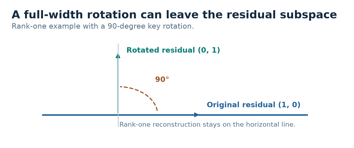
Figure 9. Original two-dimensional counterexample to pulling a full-width rotation through a generic residual basis. The horizontal line is the reconstructible rank-one subspace. A quarter turn sends the true residual outside it.

An exact decode option stores unrotated latents and computes the position-specific contraction. For a rotated query $\tilde q_i$, the private score at $j$ is

$$\tilde q_i (z_j B_h^\top D_j)^\top = (\tilde q_i D_j^\top B_h)z_j^\top .$$

The bracket now depends on key position $j$. It cannot in general be computed once for the entire query. One can expand keys in tiles, at a computational cost. An architectural alternative constrains the basis to invariant rotary subspaces, or assigns positional information a separate channel. Either choice changes the design and would need to be trained and compared. The published algebra establishes associativity for the linear core. I would require an explicit positional specification to extend it to the reported training recipe.

Post-projection normalization has a cache cost

Section 4.3 attributes the behavior of large projection norms to post-projection RMSNorm. With $k_j=s_j+z_j B_h^\top$, write its scalar denominator as $n_{h,j}$. Expanding the squared norm reveals the cross term between shared and private parts.

$$d_h n_{h,j}^{\,2} = \|s_j\|^2 + 2s_j B_h z_j^\top + z_j B_h^\top B_h z_j^\top + d_h\epsilon .$$

Dividing the two branches by separate norms generally changes the key direction. One exact option in a no-RoPE linear kernel is to compute the joint reciprocal scale once per head and token, cache it, and multiply the summed dot product by that scale. A fixed per-head affine gain can be folded into the query side in this case. A single BF16 scalar for each head and position would add $bNBTH$ bytes. Relative to dense K/V payload, that is $1/(2d_h)$ if stored at the same precision. It also adds memory traffic and append-time work. An unreported treatment of this scale makes it hard to pair the analytical memory and computation numbers with the training architecture.

The same caveat qualifies gauge invariance. The paper’s $A_h$ describes linear content logits. With position-dependent rotations the effective bilinear form depends on the relative position, and an arbitrary head rotation can alter it unless the transform commutes with the rotary action. Post-projection normalization and learned gains also restrict the invariances. Head-map PCA is informative as a standardized probe. An input-conditioned comparison of actual attention outputs and an intervention on selected heads could test whether the geometric diversity is behaviorally useful.

Reconcile the accounting before choosing a serving point

Several Appendix G entries can be checked directly. At 2.5B, Table 7 gives rank 55, which is consistent with about 48.5% payload. At rank 64, the formula instead gives $1/18+64/128=55.56\%$, exactly the ratio of the displayed 360.0 and 648.0 numbers in Table 12. Table 12 prints 48.4% beside 360.0. The rank-64 arithmetic in Appendix G.4 repeats that smaller percentage. The analogous Table 12 ratios at 128M and 6.3B are 66.67% and 53.125%, respectively. Those also match rank 64 under Eq. 9, while the percentages printed alongside them are 52.6% and 45.1%. I keep the two configurations separate. The paper does not resolve how the absolute 2.5B payload in Table 12 was obtained from the stated Table 5 layer count and 2,048-token context.

There are related comparison issues. At 128M, Table 8 lists MLA-384 at 25% while the surrounding prose gives 50%. For 6.3B LRKV, the five printed downstream scores average 40.36% rather than the table’s reported 40.2%. The discrepancies warrant consistent per-run configuration and evaluation records. They do not prevent a direct comparison of the printed per-task cells or the exact algebraic cache ratio for a specified layout.

The latency argument in Appendix F contrasts a factored LRKV contraction with a materializing MLA path. Its own text also gives an absorbed MLA contraction. Using $K_h=ZA_h^\top$, a head can compute $(q_hA_h)Z^\top$ without materializing all head keys. Values admit the corresponding absorption. Both factored methods still scan history, with different width, reuse and positional costs. Table 10’s materializing MLA complexity is a path comparison. A fair serving benchmark would test absorbed MLA and a fused LRKV kernel, with the same batch, length, dtype and positional semantics. It would report memory-controller bytes, peak allocated memory, per-token latency quantiles and throughput under equal quality constraints. Optimized GQA is another relevant point because of its regular contiguous head groups.

9. A reproducible evaluation design

Use Table 7 for the intended rank grid and label the rank-64 analyses separately. Run one comparison with the same backbone and another with the same total parameter budget. Repeat matched-cache points across seeds and several GQA groupings and MLA latent widths. Record actual parameters, fixed-target steps, training tokens and accelerator-hours. Evaluate retrieval at varied evidence depths, report ARC and HumanEval separately, and compare head-map spectra with input-conditioned behavior.

Specify the reference positions and RMSNorm, then compare full and factored logits and values on controlled inputs. Include a non-invariant rotary plane, mixed positions and near-canceling key terms. Compare with higher precision to separate algebra from roundoff. Check append after prefill at page boundaries and count physical padding, position data and normalization scales.

Separate prefill from decode and sweep history length and concurrency. Report memory-controller bytes, peak allocation, per-token latency quantiles and admitted concurrency at a fixed latency target. Record tensor strides and sharding so the traffic can be related to the shared tiles. This is a proposed design. The examples and recalculations in this review use algebra or published values.

10. Conclusion

LRKV gives head specialization a tunable cost. Its shared dense basis preserves a common set of token features, and its private codes restore head-level variation without dropping tokens. The linear score and value contractions are easy to derive and explain the analytical payload reduction. Across the reported runs, intermediate ranks give a favorable loss versus dense-cache comparison, with useful downstream evidence and task-level exceptions.

The most informative next result would tie the quality model to a fully specified positional and normalized decode path. A reconciled rank and byte table, a controlled rank sweep, and matched-quality kernel measurements would turn the current architectural result into a decision about serving. The shared-plus-private decomposition is worth retaining in that comparison because it exposes the source of each extra byte and multiply.

References

• James O’Neill, Robert Clancy, Mariia Matskevichus and Fergal Reid. Low-Rank Key Value Attention, arXiv:2601.11471v3. Method and cache equations in §3, experiments in §4 and appendices D–G, diversity analysis in appendix C, limitations in appendix H. Paper and version history