DBW: Learning the Trade-off Between SVD Pruning and Quantization

Review date: 2026-11-06 (UTC)
Author: Zhongzhu Zhou
Paper reviewed: Differentiable Bit-Widths: Co-optimizing Pruning and Quantization via SVD for Ultra-Efficient LLM Compression
Paper authors: Hankyul Kang and Jongbin Ryu
arXiv: 2610.06026
Version and date: v1, 2026-10-05

1. What I take away from DBW

I read DBW as a resource-allocation paper written in the coordinates of a matrix factorization. Its useful idea is to make deletion a precision choice. A singular component with zero bits disappears; a surviving component receives an integer precision. Rank selection and quantization therefore become coupled decisions inside the same calibration problem. The method avoids committing to a rank before it learns how accurately the retained factors can be represented.

That is a meaningful distinction in the sub-2-bit regime. A sequential pipeline may remove a direction that a later quantizer cannot recover. Conversely, retaining too many directions may force all of them into excessively coarse numerical representations. DBW lets the calibration loss negotiate that exchange. Matrix-level budgets add a second decision: an attention projection and an MLP projection need not spend the same amount of precision.

The evidence is promising within that scope. On LLaMA-2-7B, the paper reports 49.06% mean accuracy over eight benchmarks at 1.61 effective bits, compared with 39.20% for PTQ1.61 and 63.19% for FP16. Those three numbers describe both the gain and the remaining damage. Improving on another severely compressed model does not preserve the original model’s full capabilities. I would assess the method against a deployment-specific quality floor before treating the memory savings as useful.

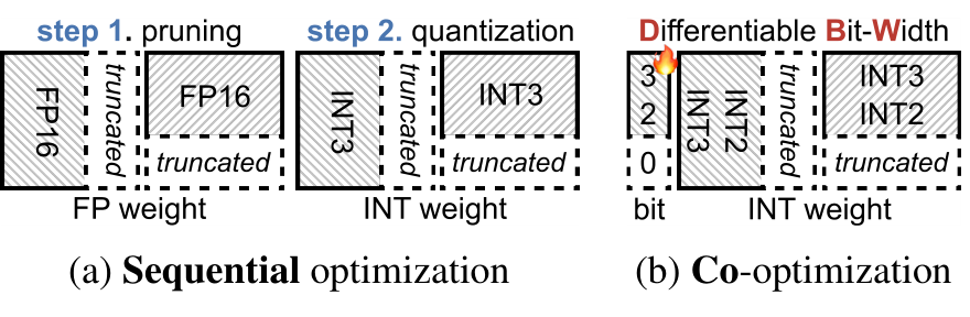
Figure 1 (paper Fig. 1): Cropped from the paper. The sequential path fixes what survives before quantizing it; the joint path makes zero and positive precisions part of one allocation. The drawing is a conceptual comparison, not an empirical error curve.

My reading covers the complete 31-page PDF: the main method, appendices A-F, and the authors’ checklist. All performance numbers below are reported by the paper unless I explicitly label an arithmetic calculation or an illustrative example. I have not run a compression experiment. The official resource is an entry point for future work.

2. Prerequisites: a rank component is an outer product

Let a linear projection have weight $W\in\mathbb{R}^{d_o\times d_i}$. Its thin SVD contains $C=\min(d_o,d_i)$ components. I use the column-vector convention for an input $x$, so the output is $Wx$. A full transformer block contains several such matrices, together with attention, normalization, residual additions, and nonlinearities.

$$W=U\Sigma V^\top=\sum_{c=1}^{C}\sigma_c u_c v_c^\top, \qquad U\in\mathbb{R}^{d_o\times C},\quad V\in\mathbb{R}^{d_i\times C}. \tag{1}$$

One component contributes an entire rank-one map. Deleting it changes both the input direction the projection observes and the output direction it writes. This is different from deleting a few individual matrix entries. At initialization, orthonormal singular vectors make the squared Frobenius error of an exact rank-$r$ truncation especially simple: it is the sum of squared discarded singular values.

$$W_r=\sum_{c=1}^{r}\sigma_c u_c v_c^\top, \qquad \|W-W_r\|_F^2=\sum_{c=r+1}^{C}\sigma_c^2. \tag{2}$$

The qualification matters. Equation (2) describes exact SVD truncation in an unweighted matrix norm. Quantized factors need not remain orthogonal, and block-level language-model loss is not the Frobenius norm. DBW also adapts factor parameters during calibration. It would be incorrect to carry the optimality of initial SVD truncation over to the entire learned system.

For input data $X$ with columns of activations, the relevant linear output error instead depends on activation covariance. Expanding the squared norm gives a useful bridge from weight reconstruction to calibration:

$$\begin{aligned} \|(W-\widehat W)X\|_F^2 &=\operatorname{tr}\!\left((W-\widehat W)XX^\top(W-\widehat W)^\top\right)\\ &=N\operatorname{tr}\!\left((W-\widehat W)C_X(W-\widehat W)^\top\right), \quad C_X=XX^\top/N. \end{aligned} \tag{3}$$

Thus a small singular value can still matter on an important activation direction. DBW uses actual block outputs to provide that task-dependent signal. Its entropy intuition should be read alongside this data dependence, rather than as a replacement for it.

3. From stored factors to a meaningful bit budget

For a retained rank $r$, two dense factors require roughly $r(d_o+d_i)$ entries, before scales, offsets, padding, or a separate singular-value vector. A full square SVD stores twice as many factor entries as the original matrix. Consequently, assigning an average bit-width to factor entries and reporting bits per original weight require different denominators.

If both vectors of component $c$ use $b_c$ bits per entry, a transparent payload calculation is

$$B_{\mathrm{payload}}=(d_o+d_i)\sum_c b_c, \qquad \mathrm{bpw}_{\mathrm{payload}}=\frac{(d_o+d_i)\sum_c b_c}{d_od_i}. \tag{4}$$

This is an accounting identity under the stated storage convention, not a claim about the authors’ exact exported layout. It excludes quantizer metadata and any transformations that change the factor dimensions. It is useful precisely because those details must be declared to interpret a reported effective precision.

For a square matrix, keeping half the components at three bits gives approximately three payload bits per original weight under Equation (4). For a tall rectangular matrix, the conversion changes again. One cannot generally multiply a surviving-component fraction by its average precision and call the answer original-weight bpw without a shape factor. The paper’s tables use effective bit and pruning-ratio summaries, while Appendix A.2 says the weight footprint additionally includes higher-precision embeddings and quantizer parameters. I retain those reported quantities separately.

There are three nested budgets. The allocation routine conserves a sum of component precision units. A serialized model consumes actual bytes. A running model also needs activations, temporary factor products, KV cache, allocator slack, and runtime workspace. DBW directly addresses the first two. Its weight-memory measurements do not establish that all resources fit into a device with the same capacity.

A useful derived check is $12.31/1.56\approx7.89$ for the reported LLaMA-2-7B weight sizes. That is smaller than $16/1.61\approx9.94$. This gap is expected when some tensors remain at higher precision and metadata is counted. It should be explained, not concealed by citing only the larger theoretical ratio.

4. Component allocation: normalize, floor, and repair

DBW gives every component a continuous parameter $\beta_c$. Positive values are normalized, multiplied by a matrix budget $A$, and converted into integer precisions. Using $a_c$ for the continuous quota and $S$ for the normalization denominator makes the mechanics easier to follow:

$$s_c=\operatorname{ReLU}(\beta_c),\quad S=\sum_i s_i, \quad a_c=A\frac{s_c}{S},\quad k_c=\lfloor a_c\rfloor. \tag{5}$$

The sum of the continuous quotas equals $A$ when $S>0$. The sum of the floors generally does not. If $A$ is an integer and all quotas are feasible, let $R=A-\sum_c k_c$. Hamilton allocation gives an extra bit to the $R$ largest fractional remainders. The resulting integer sum equals the target.

$$r_c=a_c-k_c,\qquad b_c=k_c+\mathbf{1}\{c\in\operatorname{TopR}(r)\},\qquad \sum_c b_c=A. \tag{6}$$

This equality needs an integer target, a valid normalization, and a defined policy for any upper cap. A continuous matrix-level budget is not automatically an integer, and the main equations do not specify every rounding and saturation corner case. If candidates are restricted to $0,\ldots,5$, leftover bits must go to components still below the cap. Renormalizing or redistributing after saturation changes the projection. These are specifications a future reproduction should make explicit.

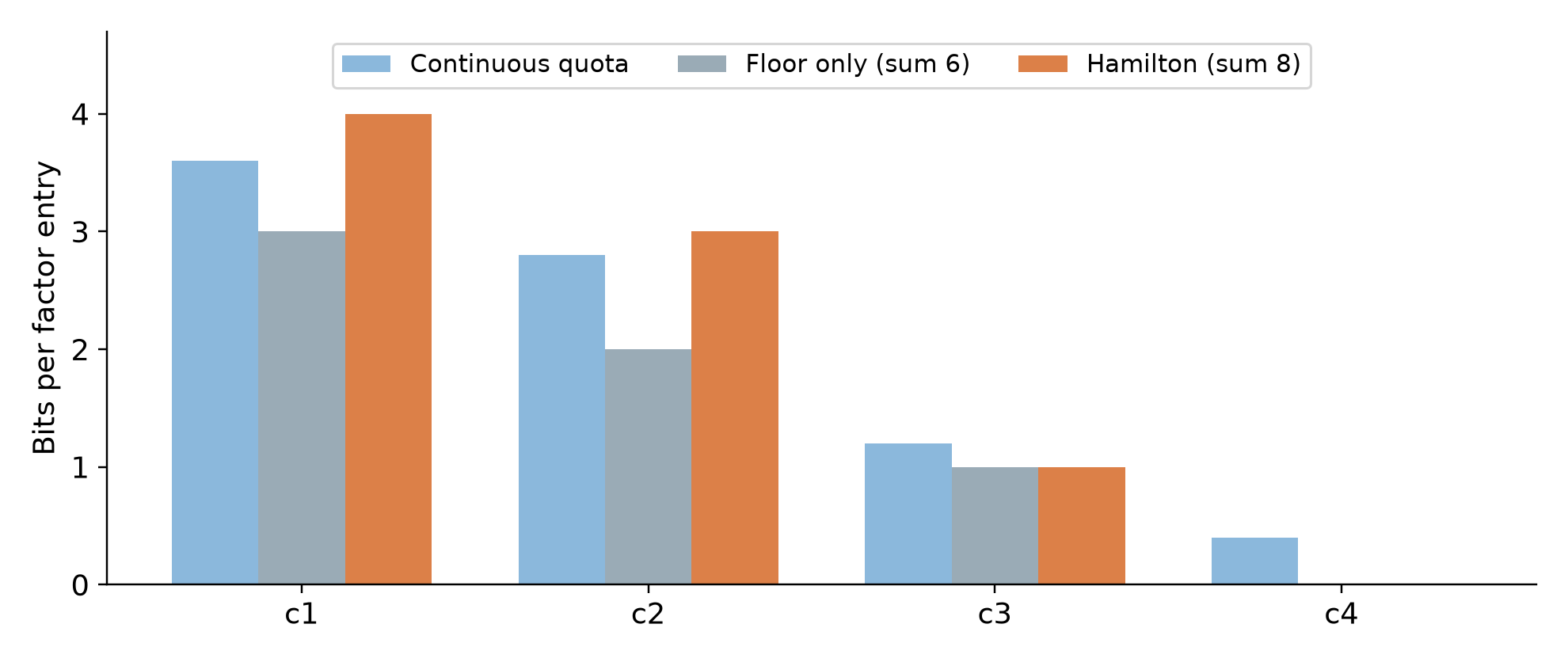
Figure 2: My illustrative arithmetic example, not a model experiment. Quotas $(3.6,2.8,1.2,0.4)$ sum to eight. Flooring spends six bits; remainders select the second and first components, producing $(4,3,1,0)$ and spending all eight.

The example also shows the pruning mechanism. The last component receives zero bits and is removed. The third survives at one bit even though it receives no leftover unit. A zero bit is a structural decision; it is not a tiny positive precision.

Algorithm 1. Integer component allocation

The following numbered pseudocode explains the forward allocation in paper Section 2.2 and Appendix C.2. The preconditions and tie rule are explicit here for clarity.

1. Input nonnegative quotas induced by beta, integer budget A.
2. Require a positive normalization sum and feasible bit limits.
3. Compute a[c] = A * relu(beta[c]) / sum(relu(beta)).
4. Set k[c] = floor(a[c]); compute remainder r[c] = a[c]-k[c].
5. Set R = A - sum(k[c]).
6. Select R feasible components by descending r; break ties stably.
7. Set b[c] = k[c] + 1 for selected components, else k[c].
8. Check sum(b) = A and all bit limits; return b.

Why use Hamilton rather than random repair? It makes the integer allocation close to its continuous quotas and deterministic once ties are defined. The paper’s Table 11 reports PPL 10.54 and accuracy 49.06 for Hamilton, versus 11.86 and 46.18 for random leftover assignment. Floor-only uses less than the intended budget, so its weaker result cannot isolate rounding quality at equal memory. The random comparison is the more informative budget-matched control.

5. What differentiability actually means here

The integer map is piecewise constant and jumps at floor boundaries or changes in remainder ranking. DBW uses a straight-through estimator (STE) to pass a surrogate gradient through these operations. It therefore learns with an approximate gradient, even though the forward values are discrete. Calling this differentiable is conventional optimization terminology, not a statement that the true discrete map has an ordinary useful derivative everywhere.

Within a region where all relevant $\beta$ values are positive, differentiating the continuous normalization exposes competition between components:

$$\frac{\partial a_c}{\partial\beta_j} =A\frac{\mathbf{1}\{c=j\}S-\beta_c}{S^2}. \tag{7}$$

Increasing one score raises its own quota and lowers the others. Multiplying all positive scores by a common constant leaves the forward allocation unchanged. This scale invariance creates a redundant optimization direction, while very small $S$ can amplify gradients. ReLU also makes negative-score recovery depend on the chosen surrogate and boundary behavior. The paper’s empirical success does not remove these numerical considerations.

Appendix C.2 observes that Hamilton changes a component’s forward precision by at most one bit. That bounds a value correction, not the error of the surrogate gradient. Near a tie, an arbitrarily small change can swap the recipient of a leftover bit. Loss sensitivity can also differ sharply between the two components. A convergence claim would need additional assumptions on that sensitivity and the discontinuities; the reported experiment establishes practical behavior on the tested settings.

6. The learned quantizer: precision enters the scale

The second part of DBW is a quantizer whose surrogate derivative can reach a bit-width parameter. For a vector or quantization group with lower bound $l$ and upper bound $h$, define $t=(w-l)/(h-l)$ and $q=2^b-1$. When $b>0$, Appendix C.3 maps the normalized value onto $q+1$ levels and back:

$$t=\frac{w-l}{h-l},\qquad q=2^b-1, \qquad \widehat w=l+(h-l)\frac{\operatorname{round}(tq)}{q}. \tag{8}$$

The bounds, grouping, and any clipping must be interpreted consistently; Equation (8) assumes $h>l$ and $t\in[0,1]$. A constant group needs a separate convention. The paper uses group size 128 in its main setting. Grouping helps adapt numerical range locally but adds scales and offsets that must be included in storage accounting.

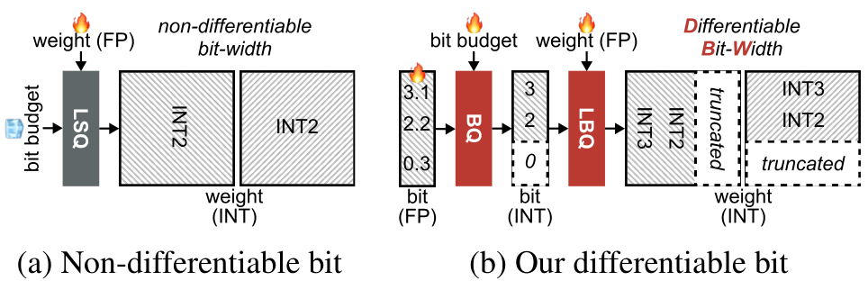
Figure 3 (paper Fig. 2): Cropped from the paper. BQ allocates integer precision, while LBQ applies that precision to the factors. The gradient route through scaling is the important distinction from simply placing a learned number inside a clipping bound.

A short derivation explains why this construction supplies a signal. Hold $t,l,h$ fixed, approximate the derivative of rounding by one, and let $k=\operatorname{round}(tq)$. Then differentiation through both the numerator and denominator gives

$$\begin{aligned} \frac{\partial\widehat w}{\partial b} &\approx(h-l)\frac{tq-k}{q^2}\frac{\partial q}{\partial b},\\ \frac{\partial q}{\partial b}&=(\ln2)2^b. \end{aligned} \tag{9}$$

The signal is proportional to a rounding residual. It is not limited to values outside a clipping range. This is my derivation of the local surrogate under the stated assumptions; it is not an exact derivative of discrete quantization. If bounds move, extrema change, or clipping is active, additional derivative terms and conventions matter.

At $b=0$, $q=0$ makes the expression undefined. DBW explicitly defines the component output as zero, rather than evaluating Equation (8). Pruning therefore requires its own forward branch. Equation (9) also shows why the transition into that branch deserves attention: the positive-bit formula contains $q^{-2}$. An exact zero branch and a smooth backward approximation do not by themselves explain how an already deleted component can recover precision.

An alternative is a soft mixture over several candidate quantizers. It can supply gradients but duplicates candidate computations and needs a later hard choice. A fixed-bit quantizer is cheaper but cannot negotiate precision. DBW’s direct scalar route is attractive for large models because it avoids maintaining a full mixture for every component. The trade-off is reliance on a chosen surrogate around discrete and degenerate cases.

7. Matrix budgets: another level of competition

A transformer block has multiple matrices. A component-only allocation may still force the same effective budget onto a sensitive MLP projection and a more redundant attention projection. DBW introduces learnable matrix scores $\alpha_m$ and normalizes them to a block budget $T$:

$$A_m=T\frac{\alpha_m}{\sum_j\alpha_j}, \qquad \sum_m A_m=T. \tag{10}$$

This is paper Equation (3), rewritten with $A_m$ for the allocated amount. As written, it assumes a nonzero denominator; valid nonnegative budgets also require appropriate parameter constraints. Appendix C.4 reports that tested matrix budgets do not collapse to zero, and explicitly calls that an empirical observation. Reconstruction error discourages destroying a necessary matrix, but it is not a formal lower-bound constraint.

There is a separate dimensional question. If $A_m$ measures original-weight bpw, a physical block constraint weights it by $d_o^{(m)}d_i^{(m)}$. If it measures a sum of component precisions, Equation (4) supplies a different matrix-dependent coefficient. A raw sum of heterogeneous quantities does not automatically conserve bytes. The weighted-average note in Table 19 is therefore essential when interpreting the empirical output. I would ask a future methodological description to state the unit of every budget before normalizing it.

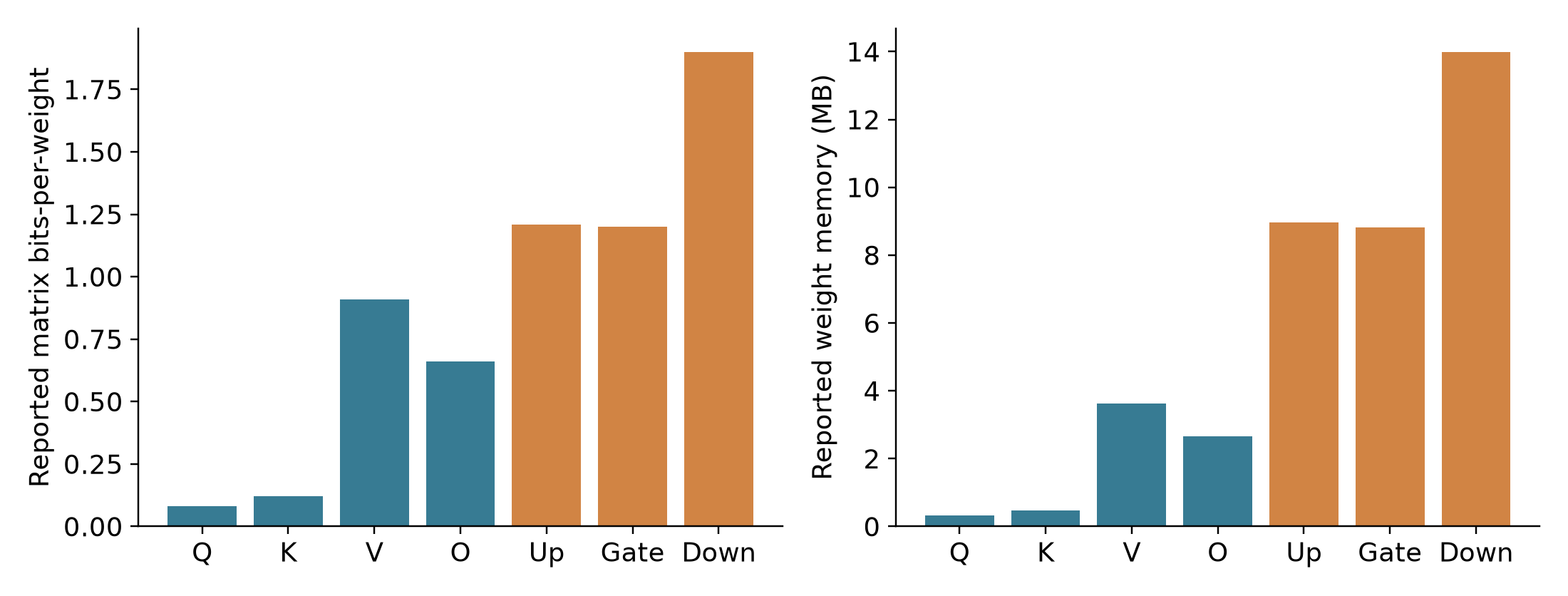
Figure 4: Redrawn from paper Table 18 for LLaMA-2-7B. Q/K receive much smaller reported bits and weight footprints than the MLP down projection. These are descriptive table values, not a proof that entropy alone predicts sensitivity.

Table 19 gives an accuracy change from 48.77% for single-level allocation to 49.06% for bi-level allocation. That is a 0.29 percentage-point improvement. It supports extra flexibility, but its scale is much smaller than the headline gain over weak uniform allocation. A sensible interpretation distinguishes the benefit of component adaptation from the incremental value of matrix adaptation.

8. Entropy regularization: useful pressure, limited certificate

DBW also learns the singular-value parameters and penalizes the entropy of their normalized nonnegative values. For positive $s_i=\operatorname{ReLU}(\sigma_i)$ and $Z=\sum_i s_i$, the objective is

$$p_i=s_i/Z,\qquad H(p)=-\sum_i p_i\log p_i, \qquad L=L_{\mathrm{rec}}+H(p). \tag{11}$$

The entropy is small when a few coefficients dominate. Concentrating the distribution makes removal of many small coefficients more attractive. This is the rationale behind the regularizer. It does not directly penalize the calibration output error, so reconstruction remains necessary to prevent a concentrated but unhelpful representation.

Differentiating in the strictly positive region gives another useful interpretation. Since $\partial p_i/\partial s_j=(\mathbf{1}\{i=j\}-p_i)/Z$, summing the chain rule yields

$$\frac{\partial H}{\partial s_j} =\frac{-\log p_j-H(p)}{Z}. \tag{12}$$

A small-probability coefficient tends to receive pressure toward further shrinkage, while dominant coefficients can grow relative to the total. The logarithm requires a convention at zero; the limit of $p\log p$ is zero, but its derivative is not numerically benign. This is another place where a mathematical definition and a stable finite-precision treatment differ.

The paper calls these parameters singular values. At initialization that is literal. If both factors later change without an orthogonality constraint, the diagonal coefficients need not equal the true singular values of the reconstructed matrix. Rescaling one factor column and inversely rescaling its diagonal coefficient can preserve the product while changing coefficient entropy. Thus low learned coefficient entropy is a useful optimization signal, but not automatically a representation-invariant certificate of low effective rank.

An alternative would regularize actual singular values of the reconstructed matrix, or maintain normalized/orthogonal factors. Either choice adds cost or constraints. A cheaper diagnostic would report column norms, the true reconstructed spectrum on selected layers, and output error together. That would show whether entropy reduction reflects meaningful compression structure or partly a change of factor scale.

9. Block calibration and the full learning loop

DBW calibrates one transformer block at a time. The reconstruction target is the original block output on sampled activations; other blocks remain fixed during the local optimization. The paper uses 4,096 RedPajama-1T sequences of length 2,048, two epochs, batch size two, Adam with cosine scheduling, learning rate $2\times10^{-5}$ for weights and component bits, and $10^{-4}$ for matrix bits. Appendix A describes a subsequent quick quantization-parameter calibration to reduce inter-block distribution shift.

$$L_{\mathrm{rec}}=\frac{1}{|\mathcal{X}|}\sum_{X\in\mathcal{X}} \|f(X;\widehat\Theta)-f(X;\Theta_{\mathrm{ref}})\|_F^2. \tag{13}$$

Here $f$ is a whole block, so the loss includes interactions among its projections and nonlinearities. The reference weights are fixed in this notation; the learnable factors produce $\widehat\Theta$. The averaging convention can include token and feature dimensions. Its scale matters relative to an unweighted sum of entropy terms across matrices. The paper states a summed objective, but a reproduction needs those reductions specified to interpret the effective strength of regularization.

Algorithm 2. Blockwise DBW calibration and export

This is an explanatory expansion of paper Algorithm 1, with export operations described in Section 2.3. It describes a procedure rather than reporting an execution.

1. Cache calibration inputs and fixed reference outputs for a block.
2. Initialize each projection with SVD factors and bit scores.
3. For each calibration update, normalize matrix budgets.
4. For each matrix, allocate integer component bits with Algorithm 1.
5. Quantize both factor vectors; zero-bit components contribute zero.
6. Evaluate the compressed block on the same calibration inputs.
7. Sum block reconstruction loss and coefficient entropy losses.
8. Update factors, coefficients, and bit scores using surrogate gradients.
9. Finish the block and apply the stated quick parameter calibration.
10. Group retained components by bit-width and pack their factors.
11. Store ranges, offsets, dimensions, and group boundaries for inference.
12. Continue to the next block; evaluate the complete compressed model.

Local calibration saves accelerator memory and permits the reported 24GB RTX 3090 setup with 256GB host RAM. It does not make the whole process a zero-cost transformation. Two epochs expose 8,192 sequences per block, as Table 9 notes; this is repeated local work, not 8,192 total sequences of compute for the entire model. End-to-end training could address interactions across blocks, but would increase memory and compute requirements. A smaller inter-block correction pass is an intermediate option.

10. Export and inference: two factored products per group

After calibration, sorting components by bit-width makes the irregular precision pattern into a small collection of dense groups. For an input matrix $X\in\mathbb{R}^{d_i\times n}$, let $\mathcal{C}_b$ be the components assigned $b$ bits. Their contribution can be evaluated as a narrow intermediate followed by an output projection:

$$Z_b=\widehat V_b^\top X,\qquad Y=\sum_{b>0}\widehat U_b\Sigma_b Z_b. \tag{14}$$

The diagonal scale can be absorbed into a factor’s dequantization parameters as the paper describes. The two products within a group remain dependent: $Z_b$ must exist before the corresponding output multiplication. Across groups, independent work can overlap before partial outputs are accumulated. Sorting must apply the same permutation to both factors and their coefficients; otherwise it changes the represented matrix.

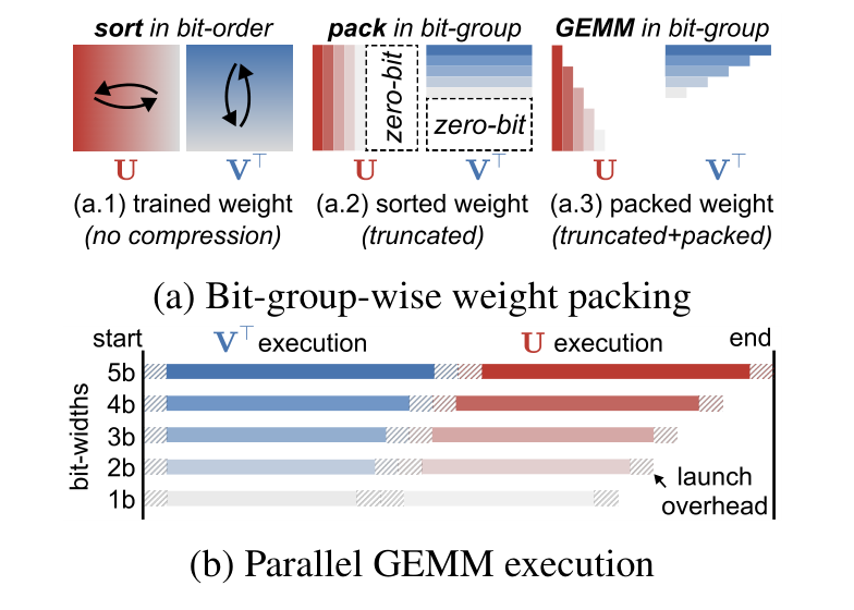
Figure 5 (paper Fig. 3): Cropped from the paper. Equal-precision components are packed together. The execution diagram also exposes a cost: each nonempty group introduces work and launch scheduling even when its rank is small.

The arithmetic count for the two factored products is approximately $2nr(d_i+d_o)$ FLOPs, compared with $2nd_id_o$ for the dense projection. Under this convention, factorization reduces multiplication count only when

$$r<\frac{d_id_o}{d_i+d_o}. \tag{15}$$

For a square matrix this means $r<d/2$. Removing components is therefore not sufficient by itself to guarantee fewer FLOPs than the original dense matrix. For rectangular projections the threshold changes. Effective numerical precision can reduce weight traffic without reducing floating-point multiply count; these benefits should be measured separately.

The paper describes weight-only quantized GEMM with on-the-fly dequantization and floating-point computation. It does not imply that a GPU executes arbitrary 3-bit tensor-core matrix products natively. Appendix C.5 explains a packing strategy that splits non-dividing widths such as three bits into two-bit and one-bit planes, then combines them during unpacking. The extra bit manipulation is small when matrix multiplication dominates, but becomes visible when each group has little work.

An alternative is reconstructing a dense weight before multiplication. That makes the computation conventional but loses persistent compressed-weight traffic and can require a large temporary tensor. Another alternative is a fused grouped kernel that avoids repeated launches. The paper identifies fusion as future work; its reported CUDA-stream grouping should not be described as an already fused inference engine.

11. Experimental design and the strongest comparisons

The main evaluation covers LLaMA-1/2/3 models from 7B to 70B. It measures WikiText-2 and C4 perplexity at sequence length 2,048 and mean zero-shot accuracy across PIQA, ARC-Easy, ARC-Challenge, HellaSwag, WinoGrande, RACE, and two LAMBADA variants. Appendix A.2 identifies lm_eval 0.4.2 and Transformers 4.40.1 for the reported setup. These details matter because prompt construction and evaluation conventions can move the accuracy scale.

The eight-task mean weights the benchmarks equally. It is not a measure of long-form reasoning reliability, calibrated confidence, instruction following, or agent success. Table 2’s arithmetic means over available model sizes exclude missing or NaN entries. A baseline with missing large-model results may therefore have an average over a different set of models; row-wise comparisons are easier to interpret than the aggregate alone.

Table 5 is more directly relevant to the central claim than a comparison with an unrelated pruning method. It places sequential SVD-plus-quantization and DBW at similar reported bpw and weight memory. For LLaMA-2-7B, SVD-LLM plus OmniQuant reports PPL 77.10 and accuracy 29.35, while DBW reports 10.54 and 49.06 at 1.56GB. This is a large practical difference in the configurations tested.

It is still a comparison of pipelines with different degrees of freedom and optimization. DBW learns bit assignments, matrix allocations, and coefficients with a block reconstruction objective. A matched baseline that used the same calibration compute, trainable targets, and range adaptation while fixing only rank selection would more cleanly isolate joint allocation. The paper’s controlled factor experiments move in that direction, but do not reduce all differences to one switch.

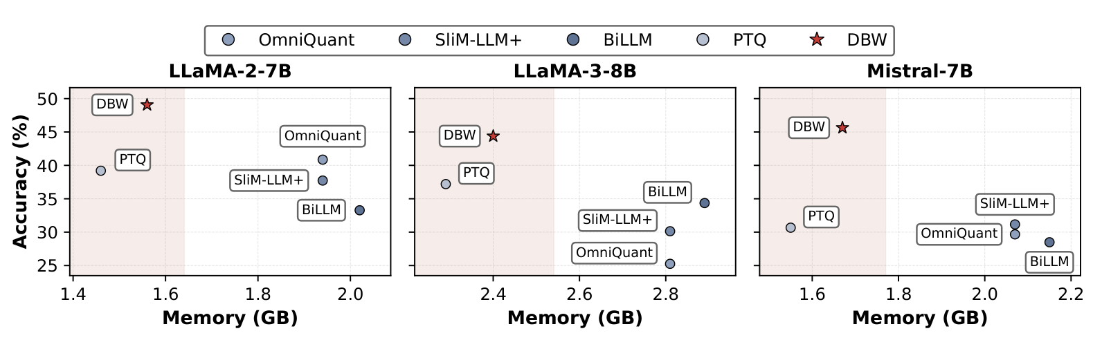
Figure 6 (paper Fig. 4): Cropped from the paper. DBW occupies a favorable region of the measured weight-memory/accuracy plane for these settings. The axes concern model weights and a benchmark mean; they do not include runtime cache capacity or prove a universal Pareto frontier.

Table 6 compares structured-pruning baselines that retain FP16 weights against DBW’s low-bit factors. Matching pruning ratio is useful for studying structural reduction but does not match stored bytes. The table reports memory explicitly, which should remain part of any interpretation. It cannot establish that SVD structure alone explains the entire quality advantage at identical deployment cost.

12. Absolute quality and the bit-rate curve

For LLaMA-2-7B, the most informative compact view is Table 3. Moving from 2.0 to 1.61, 1.0, and 0.5 reported bits trades quality for more compression. The following values reproduce that table; PPL is the arithmetic mean of WikiText-2 and C4 perplexities, rather than a pooled-corpus perplexity.

Setting	Reported bits	Mean PPL	Eight-task accuracy (%)
FP16	16	6.22	63.19
DBW	2.0	9.56	51.90
DBW	1.61	10.54	49.06
DBW	1.0	14.97	39.66
DBW	0.5	27.68	30.93

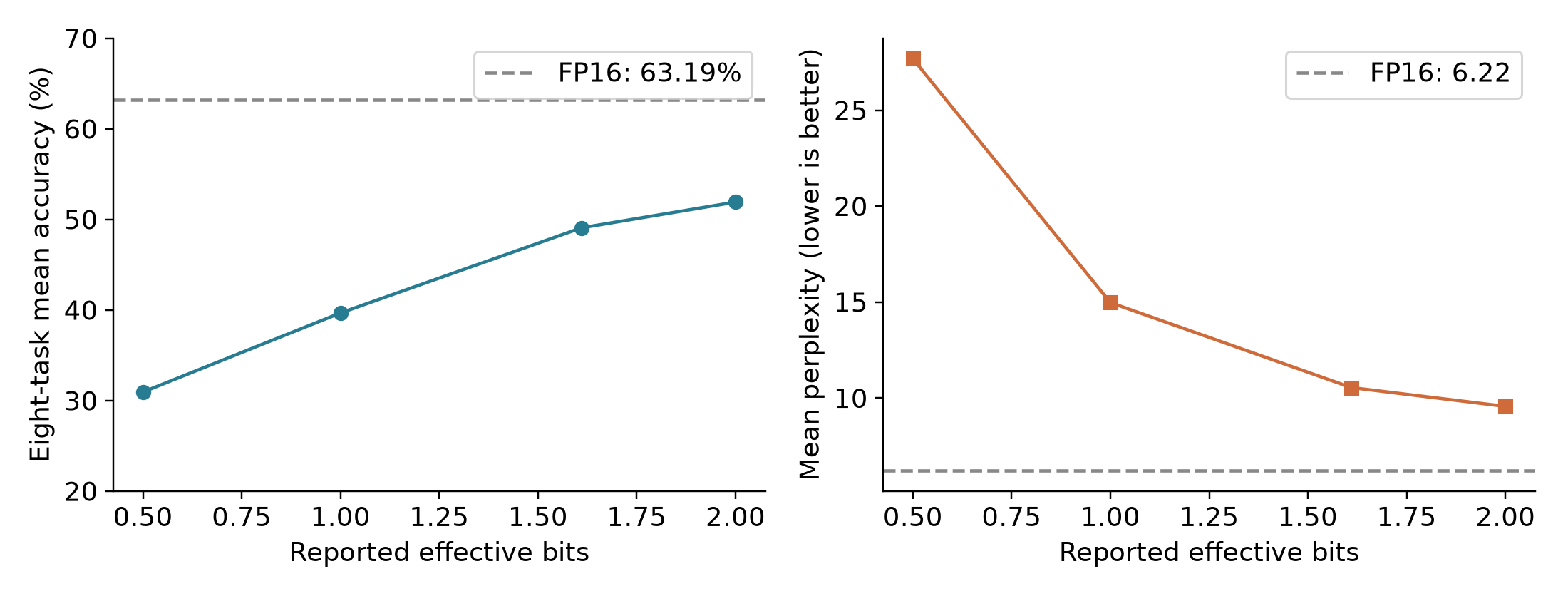
Figure 7: Redrawn from paper Table 3. The FP16 reference makes the absolute degradation visible. The line segments connect sampled settings for readability; they do not represent measured intermediate configurations.

At 1.61 bits, the gap from FP16 is $63.19-49.06=14.13$ percentage points, calculated from the table. The improvement over PTQ1.61 is $49.06-39.20=9.86$ points. Both are true. Reporting only the second would obscure the loss that a downstream user must accept. Perplexity also rises from 6.22 to 10.54, although a ratio of arithmetic-mean perplexities should not be interpreted as a direct token-error ratio.

Appendix D.2 makes the reasoning limitation even clearer. At 1.61 bits, DBW’s LLaMA-2-7B GSM8K accuracy is 2.12%, compared with 0.61% for PTQ1.61. That is an improvement within an extremely low-performance regime. The corresponding MMLU value is 23.89%. These results are insufficient to claim preservation of sophisticated mathematical reasoning or a dependable reasoning assistant.

Transfer beyond LLaMA is mixed in absolute terms. Table 4 reports Gemma-7B mean PPL increasing from 8.82 to 74.49 and accuracy falling from 66.37 to 30.27. DBW is better than the tested BiLLM result, yet substantial damage remains. Mistral-7B and Qwen-2.5-7B provide additional evidence of applicability, but a small set of models does not establish an architecture-independent behavior law.

Instruction-tuned and distilled models in Table 14 broaden the study. They show that the procedure can operate after post-training. Their reported benchmark mean still does not directly test whether conversational alignment, tool selection, refusal behavior, or structured output survives. Those are meaningful next measurements when compression is used in an agent system.

13. Allocation ablations: what contributes how much?

The contrast between uniform and learned allocation is dramatic, but the stronger static heuristic is the right reference for the incremental learning claim. Table 7a gives LLaMA-2-7B accuracy 25.05 for uniform, 45.10 for an SVD-aware heuristic, and 49.06 for learned allocation. The gain over the heuristic is 3.96 points; most of the gain over uniform already appears once allocation respects component importance.

Table 7b further distinguishes trainable targets. Learning component bits alone gives PPL 11.01 and accuracy 48.42. Adding matrix budgets gives 10.74 and 48.80. Adding singular-value adaptation gives 10.54 and 49.06. These are progressively smaller increments than the full uniform-to-learned comparison. For LLaMA-1-7B, the final coefficient adaptation improves accuracy but slightly worsens PPL from 10.54 to 10.65. Different metrics need not agree.

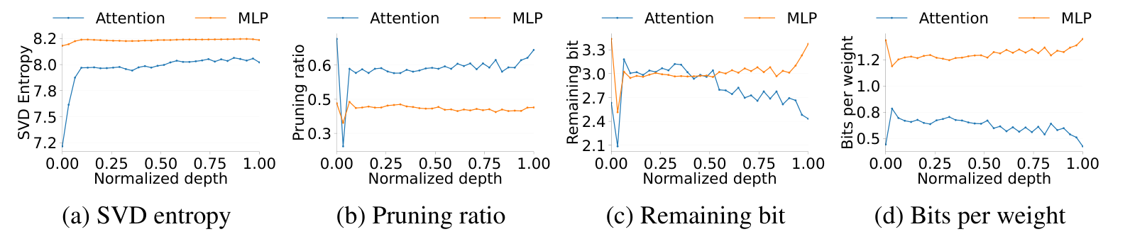
Figure 8 (paper Fig. 13): Cropped from the paper. Attention and MLP differ in entropy, pruning, retained precision, and effective bits. These curves demonstrate heterogeneity; they do not isolate entropy as the causal driver because output sensitivity and optimization also vary.

Appendix D.3 searches sequential baselines over pruning ratios and remaining precisions. This strengthens the comparison beyond one arbitrarily chosen sequential setting. At the extreme 0.5-bit target, a sequential configuration with 0.77 reported bits obtains PPL 21.62 versus DBW’s 27.68 at 0.50. It uses more budget, so this is not a matched-rate defeat. It does demonstrate why comparisons need both quality and rate instead of a single number.

Appendix A.4 repeats calibration with three seeds for LLaMA-2-7B: mean PPL 10.58 with standard deviation 0.04, and mean accuracy 49.32 with standard deviation 0.23. The stated confidence half-widths are 0.09 and 0.57. These are consistent in scale with a small-sample interval, but the paper does not fully spell out its construction. Three seeds on one model are useful stability evidence, not uncertainty estimates for every benchmark or for cross-model generalization.

There are also small reporting inconsistencies worth keeping visible. Appendix C.6’s prose says BiLLM PPL changes from 35.60 to 39.55, whereas Table 13 gives 33.10 at group size 128. Table 16’s 1.61-bit row uses pruning ratio 47.21 while Table 17 lists 46.95 for LLaMA-2-7B. I use the labeled table values in each comparison and do not infer an undocumented correction.

14. Latency is a property of a workload and a device

Figure 5 reports LLaMA-65B latency on the stated RTX 3090 setup, averaging 30 repetitions after ten warm-ups. Its horizontal axis is context length 64-512. DBW is slightly slower than OmniQuant at 64 tokens, then becomes faster as the amount of work grows. At 512, the figure annotates cuBLAS as 2.8 times DBW’s latency and 1.8 times OmniQuant’s latency. The two annotated factors use cuBLAS as a common reference; 2.8 is not DBW’s speedup over OmniQuant.

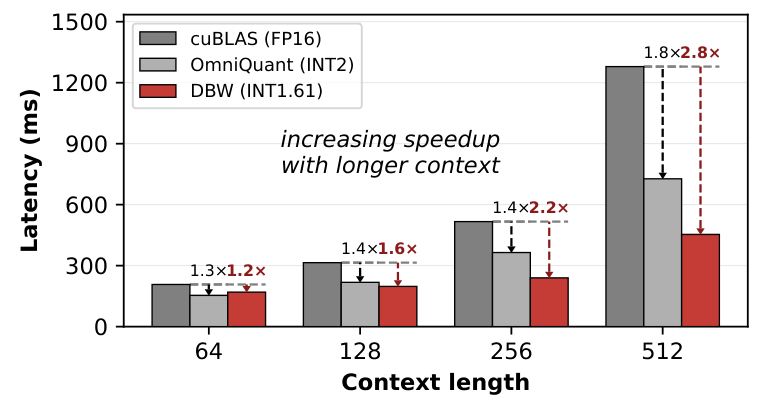
Figure 9 (paper Fig. 5): Cropped from the paper. The result is specific to the evaluated model, GPU, and timing procedure. The short-context crossover is part of the evidence and should accompany the best speedup.

Using the annotated factors, the derived DBW speedup over OmniQuant at 512 is approximately $2.8/1.8\approx1.56$. This is arithmetic from rounded figure labels, not an independently timed result. Reporting its exact-looking decimals would imply more precision than the source provides.

Appendix A.2 identifies a 24GB RTX 3090, while Table 17 gives an FP16 LLaMA-65B weight footprint of 121.11GB. Those full FP16 weights cannot all reside in that device simultaneously. The paper describes its result as end-to-end latency, but the provided text does not fully reconcile weight residency, any layerwise staging, and how the FP16 reference is timed. I would request that clarification before extrapolating the result to a fully resident production service.

A useful diagnostic model, rather than a fitted model of the paper, is to decompose latency into weight transfer, arithmetic, dequantization, launches, and output reduction. More retained groups increase launch and reduction costs; more tokens amortize weight reads but raise arithmetic demand. This explains why a single bpw value cannot predict latency and why Table 12’s INT3 runtime can be slower than INT4 despite its smaller payload.

The paper does not provide a comprehensive service-level experiment with varied concurrent users, KV-cache pressure, time-to-first-token, inter-token latency percentiles, and long-running throughput. Its compression and GEMM evidence can motivate that work. It should not be converted into an unmeasured claim about requests per second or total serving cost.

15. Limitations acknowledged in the paper

Appendix F identifies the central scope boundaries. Training is blockwise and does not explicitly optimize global inter-layer interactions. The study focuses on the sub-2-bit regime and language models. It treats weights rather than activation or KV-cache quantization. The main text also calls for testing across vision, speech, and multimodal architectures.

The hardware treatment remains a prototype-level grouping strategy with room for fusion. A small positive rank per bit group can be inefficient even when every group is mathematically dense. Weight-memory reduction leaves runtime state untouched, so long-context inference may become cache-bound after the weights shrink. The optimal compression point can therefore change with the serving workload.

Calibration uses general text, which may underrepresent code, rare tokens, mathematical states, or application-specific prompts. Local output MSE is a practical objective but does not impose a guarantee on the tails of a distribution or on discrete behavioral failures. The reported post-trained model evaluations reduce some uncertainty without covering all those behaviors.

16. Critical analysis: what would make the argument sharper?

16.1 State a byte-conserving optimization problem

The most valuable clarification would be an explicit map from each scalar budget to stored bytes. Matrix dimensions, factor ranks, bit-plane packing, quantization groups, offsets, embeddings, and padding all affect the result. A shape-weighted budget can still be normalized and learned, but its units must remain consistent across projections.

I would report both a logical allocation residual and a serialized-byte residual. The first checks Hamilton’s integer sum. The second checks the actual storage target. This distinction would resolve whether a successful precision allocation also solves the advertised memory-constrained problem. It is a methodological improvement, not evidence that the reported memory measurements are false.

16.2 Separate forward rounding error from gradient quality

An extra bit per component is a bounded value correction. It does not bound the optimization error after a discontinuous top-$R$ decision. A useful study would compare Hamilton with a smooth relaxation during learning while using identical discrete export and equal final bytes. It should report bit-assignment turnover near ties, loss jumps, and the fraction of components stuck at zero.

The essential question is whether the surrogate directs scarce precision toward components that matter to the block, especially as scores cross discrete boundaries. Final PPL alone can hide unstable trajectories that happen to end well. Conversely, a stable but biased allocation could be adequate in practice; the experiment should establish which situation occurs.

16.3 Test whether entropy tracks intrinsic structure

The entropy rationale is plausible at SVD initialization. After factor adaptation, coefficient entropy may be affected by factor scaling. I would compare coefficient entropy with the true spectrum of selected reconstructed matrices and with their activation-weighted error. A normalized-factor variant would test whether the regularizer’s benefit persists after removing scale freedom.

That comparison would also distinguish correlation from mechanism. MLP matrices may receive more budget because of nonlinear sensitivity or activation distribution as well as their spectrum. An intervention that changes entropy while holding output sensitivity approximately fixed would strengthen the causal interpretation.

16.4 Measure quality where users experience failure

The low GSM8K values make absolute quality a first-class constraint. I would define a minimum score on representative mathematical, code, and instruction tasks, then minimize bytes subject to that floor. Equal-rate plots remain useful, but they answer a different question from the least costly configuration that still meets an application’s needs.

At least one set of held-out calibration-domain shifts would be valuable. For example, compare general-text calibration with mixed text/code/math calibration under the same token and update budget. Report worst-task drops, structured-output validity, and generated-answer quality alongside the eight-task mean. Those are proposed experiments; none were run for this review.

16.5 Clarify the actual latency experiment

The FP16 residency question, exact meaning of context length, measured phases, and any host-device transfers should be stated together. A resident smaller-model baseline on the same GPU would be a useful companion to the large-model comparison. Matched-quality configurations would show whether DBW’s speed advantage remains after spending enough bits to satisfy a common quality floor.

For serving, I would vary batch size, prompt length, generated length, and available cache memory, then report weight bytes, peak allocated memory, and latency percentiles. This would locate the crossover where extra groups or cache pressure erase an otherwise attractive weight compression benefit. The paper’s short-context slowdown already suggests that such a crossover is real.

17. Reproduction notes and decision criteria

A future reproduction should begin with the paper-defined data and calibration conditions: model family and variant, 4,096 sequences of length 2,048, two epochs, group size 128, the two learning-rate scales, and the stated evaluation versions. It should keep original reference outputs fixed and document whether each block sees original or progressively compressed upstream activations. That choice changes the distribution the reconstruction objective learns.

The mathematical specification should declare the units of $T$ and $A_m$, integer conversion, bit caps, tie handling, normalization at zero, constant quantization groups, and the zero-bit backward convention. It should also declare MSE reduction and entropy scaling. These details are necessary to interpret the method independently of a particular software package.

For evidence, I would retain per-task accuracy, both perplexities, actual serialized weight bytes, peak runtime memory, and timing phase definitions. Calibration-seed variation should accompany at least the main comparisons. My arithmetic checks above verify relationships among reported numbers; they do not constitute a reproduction of the models or kernels.

18. Conclusion

DBW’s strongest contribution is a useful formulation: a rank component can compete for zero or positive precision, and the same calibration objective can decide both rank survival and quantization resolution. Hamilton repair makes the forward integer allocation precise under its assumptions; LBQ supplies a surrogate signal through the quantization scale; matrix budgets and coefficient adaptation provide additional flexibility.

I find the controlled comparisons sufficient to make joint allocation worth further study in aggressive weight compression. I would keep four caveats attached to that conclusion: budget units must be tied to bytes, approximate gradients need a narrower interpretation than convergence guarantees, low coefficient entropy is not automatically an invariant spectral property after factor learning, and improved compressed-model quality still leaves large absolute capability losses. A deployment decision needs those facts alongside the best compression and speedup numbers.

References

1. Hankyul Kang and Jongbin Ryu. Differentiable Bit-Widths: Co-optimizing Pruning and Quantization via SVD for Ultra-Efficient LLM Compression. arXiv:2610.06026v1, 2026. Primary source for all method details, tables, figures, and appendices discussed here.
2. DBW paper HTML, including appendices A-F. Figure numbers and table numbers in this review refer to this paper.
3. Official DBW resource, linked by the authors. Resource entry only; this review reports paper analysis and no newly executed model experiments.