iS-KV: When the Basis Moves, the History Must Move with It

Review date: 2026-10-30 · Author: Zhongzhu Zhou
Paper reviewed: iS-KV: Online Low-Rank KV Cache Compression via Block-Incremental SVD
Paper authors: Yiren Zhao, Guanghui Song, Tianrui Qin, Kejiang Ye, Cheng-zhong Xu, Xitong Gao
arXiv: 2610.02815 · Version: v1, 2026-10-02

1. The question is how to preserve a changing representation

iS-KV compresses the KV cache during autoregressive inference. It does not train the language model, and it is not a lossless attention algorithm. Its promise is more specific: retain every token position, keep selected and recent states exact, and represent older states with fewer coordinates. Later queries can still address the entire history, although the reconstructed vectors may differ from their original values.

That distinction matters for reasoning. Deleting a token removes its representation altogether; a low-rank approximation keeps a potentially useful direction but may discard other information from that token. Neither choice guarantees the original answer. The paper tests whether approximation is a better trade than eviction at comparable persistent memory, rather than proving that retaining positions is sufficient for preserving reasoning.

The main technical challenge appears when the low-rank space evolves. An old coordinate vector only has meaning relative to its basis. If new tokens change that basis, leaving the old coordinates untouched silently changes the old states. iS-KV applies classical block-incremental SVD to update the basis and historical coordinates together. The useful contribution is the cache policy and its reasoning evaluation, not a new SVD primitive.

The strongest headline is an accuracy–storage tradeoff. On DeepSeek-R1-Distill-Llama-8B, rank 128 reaches 82.6% MATH-500 accuracy against 83.6% for the original model, with 4.06 times smaller persistent KV storage. On Qwen3-8B, rank 96 reaches 89.2% against 94.4%, at 5.64 times compression. Those numbers describe different models and operating points; they should not be combined into one universal claim.

The systems result is equally important: the evaluated implementation reconstructs dense KV tensors and is slower in the reported timing test. Smaller persistent storage is demonstrated; peak-device-memory savings and higher throughput are not. This review develops the mathematics, then asks where the evidence supports a practical deployment decision. All experimental numbers below are reported by the paper. Constructed examples and arithmetic are explicitly labeled; no model experiments were run for this review.

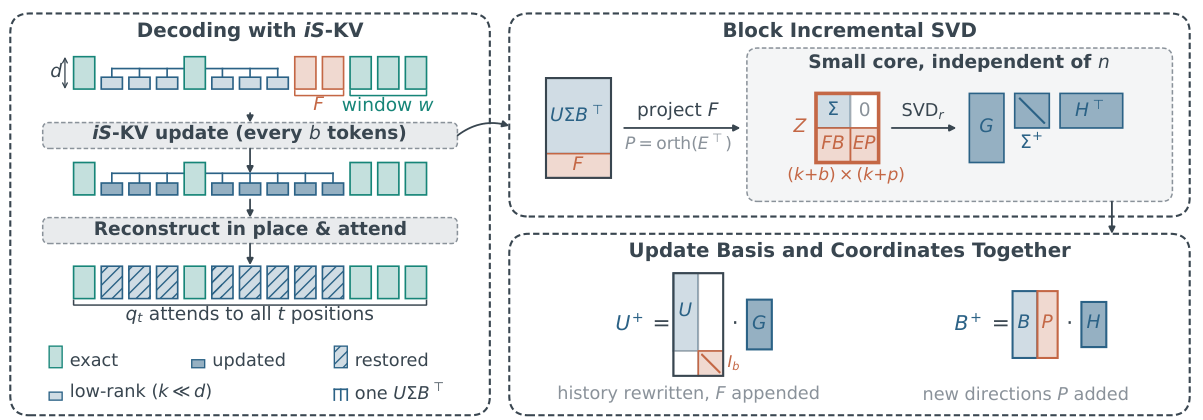
Figure 1 (paper Fig. 2, cropped). Exact recent rows feed a pending block; the block updates both the historical coefficients and the shared basis. Attention subsequently reconstructs the cache in token order. Source: Zhao et al., arXiv:2610.02815v1, p. 4.

2. Prerequisites: attention, rank, and two kinds of compression

2.1 What the cache stores

At one layer, let the sequence length be $L$, the number of KV heads be $H_{kv}$, and each head width be $D$. The paper concatenates KV heads along the feature dimension, giving $d=H_{kv}D$ and matrices $K,V\in\mathbb R^{L\times d}$. A row corresponds to a token position. The factorization is across this concatenated feature space, not an independent rank budget of the same size for every head.

For one head, attention uses a rotated query and rotated keys:

$$a=\operatorname{softmax}\!\left(\frac{q^{rot}(K^{rot})^\top}{\sqrt D}\right),\qquad o=aV. \tag{1}$$

The cache prevents repeatedly recomputing historical keys and values. It does not eliminate the need to read those states for each query. Reducing storage can improve capacity, but reducing latency additionally requires that reading, reconstructing, and updating the representation fit the hardware well.

Token eviction reduces the number of rows. Quantization reduces bytes per scalar. Low-rank compression reduces coordinates per row by sharing feature directions across positions. These choices can in principle be combined, but combinations require their own quality and systems evaluation. iS-KV does not establish that arbitrary low-bit quantization or a serving scheduler can be added without changing its conclusions.

2.2 A row is coordinates plus a shared dictionary

For the $n$ compressed rows of either path, write the maintained approximation as $A=U\Sigma B^\top$. Here $U\in\mathbb R^{n\times k}$ and $B\in\mathbb R^{d\times k}$ have orthonormal columns in exact arithmetic, while $\Sigma$ holds $k$ singular values. The effective rank satisfies $k\leq r$, where $r$ is the configured budget. A token’s coordinates are a row of $U\Sigma$; $B$ is the shared dictionary.

The truncated SVD solves the Frobenius reconstruction problem for the matrix supplied to it:

$$\min_{\operatorname{rank}(\widehat X)\leq r}\|X-\widehat X\|_F^2 =\sum_{i>r}\sigma_i(X)^2. \tag{2}$$

This criterion measures squared vector error summed across rows and features. It does not directly minimize attention-logit error, answer error, or generation length. A small singular direction can still matter to a particular future query. Thus an optimal low-rank reconstruction is a well-defined surrogate, not an optimal reasoning policy.

If a full basis changes only by an orthogonal rotation $R$, then $B^+=BR$. The same represented matrix is recovered by changing coordinates from $C=U\Sigma$ to $C^+=CR$, because

$$C^+(B^+)^\top=CRR^\top B^\top=CB^\top. \tag{3}$$

Keeping $C$ unchanged instead produces $CR^\top B^\top$. Even when the subspace is identical, the result can be wrong. When the subspace itself changes and rank is truncated, exact preservation is generally impossible; the objective becomes the best local approximation under the available budget.

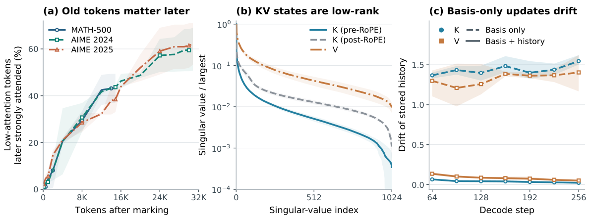
Figure 2 (paper Fig. 1, cropped). Later attention to previously low-attention tokens, normalized spectra, and the stale-coordinate failure. Bands are observed ranges, not confidence intervals. Source: paper p. 2 and Appendix A.3.

2.3 What the motivation probes do and do not show

For the attention-revival probe, the authors select the longest trace for each model and dataset. At step 1,024, they mark the bottom 75% of tokens by average attention during the previous 32 steps. A marked token counts as strongly attended later when its layer-15 attention exceeds $25/n$, where $n$ is the visible length. No token is actually removed. The reported roughly 30% revival by 8K and roughly 60% by 30K on AIME motivate preserving access; they are not measured answer losses from an eviction intervention.

The spectrum probe uses four 8K AIME 2024 traces per model, normalizes singular values by the largest, and aggregates medians over layers and traces. Pre-RoPE keys decay faster than post-RoPE keys and values. This supports where to factorize, but does not make all models or tasks equally compressible.

The third probe changes the update rule. At step 256, basis-only drift is 1.55 for keys and 1.40 for values; coordinated updates reduce it to 0.023 and 0.051. These are errors relative to the represented history before an update. They are neither final-answer errors nor the excess-error diagnostic introduced later in Appendix A.5. Maintaining that distinction prevents three different notions of fidelity from being conflated.

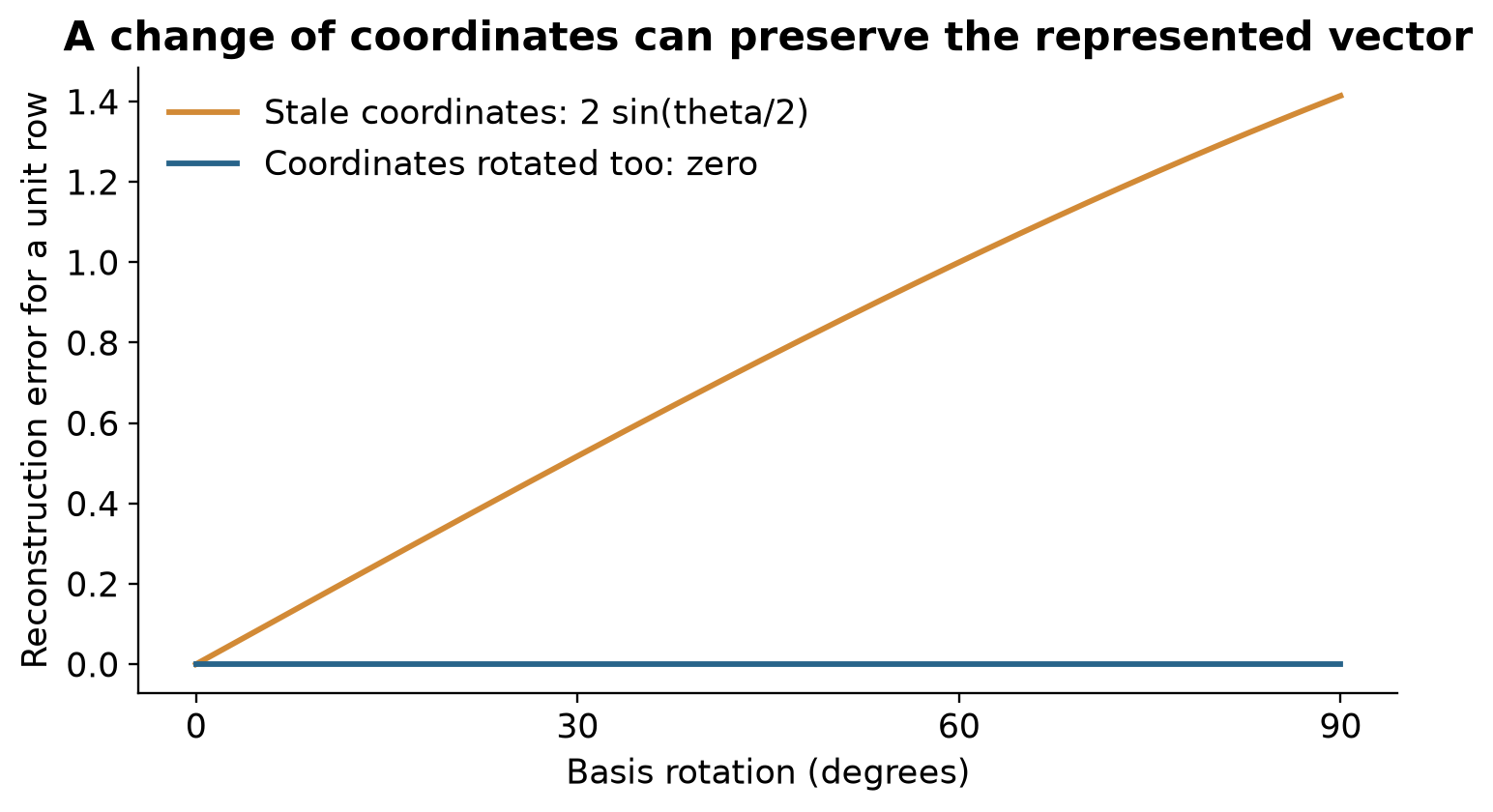
Figure 3. Constructed two-dimensional rotation example. A unit row with stale coordinates incurs error $2\sin(\theta/2)$ when the full orthonormal basis rotates by $\theta$; rotating its coordinates as in (3) preserves it. This is analytic geometry, not a paper experiment.

3. Exact states, pending states, and compressed history

3.1 Prefill chooses what stays exact

Prefill attention itself is exact: compression is applied to the cache used by later decoding. The keys are stored and factorized before RoPE, while prompt outlier selection is performed after RoPE. Position indices are retained so that reconstructed keys receive the correct rotation later. These two uses of RoPE serve different purposes and should not be interchanged.

Prompt keys are grouped into eight-token chunks. The last four chunks and any incomplete final chunk form a local suffix. For each KV head, a chunk score is the minimum cosine similarity between a token key and the chunk mean. The 128 lowest-scoring chunks per head, or all available chunks for a short prompt, are selected. The union across heads plus the suffix forms the protected key positions. Each selected position retains its complete pre-RoPE row across all KV heads.

Values within 32 positions of any protected key position remain protected. The latest 128 prompt values additionally initialize the exact recent window. Protected prompt sets are fixed during decoding, whereas recent windows advance. This design protects unusual prompt states and their local context, but a union across heads and value-neighborhood expansion can retain many exact rows. The protection overhead is therefore data dependent.

For the short MATH prompts, the rule normally protects the whole prompt. Consequently, those experiments predominantly assess compression of generated states. The 64K RULER evaluation tests a different regime: part of the prompt is already compressed when decoding begins. A headline reasoning result cannot substitute for the long-prefill retrieval test.

Algorithm 1. Initialize the cache after exact prefill

1. Compute ordinary causal prefill attention on the prompt.
2. Score post-RoPE key chunks separately for each KV head.
3. Form P_K from selected chunks and the local suffix.
4. Form P_V by extending P_K by 32 positions on either side.
5. Set W_K empty; W_V contains the last min(128, L) values.
6. For X in {K, V}, form exact positions E_X = P_X union W_X.
7. Keep X[E_X] exact; factorize the remaining rows with rank r_X.
8. Store original positions, factors, and empty pending queues.
9. Mark the initial value refit as pending; reset update counters.

Step 5 follows the displayed Algorithm 1 in the paper, consistent with the separate key/value initialization described in Section 3.1 and Appendix A.1. The paragraph preceding that algorithm loosely describes both windows as initialized from the suffix, although its displayed pseudocode leaves the key window empty. Protected key suffix positions still remain exact. This is a small specification inconsistency worth resolving before an independent reimplementation.

3.2 Decoding batches old rows without deleting positions

A new key and value enter exact storage. Once an unprotected position leaves its recent window, it enters a pending FIFO. Pending rows remain exact until there are enough to fold. The main configuration uses a 128-row recent window and 64-row regular folds; an incomplete block is retained exactly. The residual threshold does not decide when an update happens. Queue occupancy decides timing; the threshold only decides which new feature directions enter the basis.

Values have a special first fold. After $r_V$ eligible value rows have accumulated, the method reconstructs the existing compressed prompt-value history, appends those rows, and computes a fresh truncated SVD. Subsequent value folds use 64-row block updates. Thus changing $r_V$ changes both the target rank and the initial refit batch size. A rank sweep is not perfectly isolated from this initialization policy.

Keys and values may have different exact and compressed position sets. They must be scattered back into the same original token order before attention. Compressing both into contiguous matrices and pairing rows by compact-storage offset would be incorrect: a protected key does not imply the corresponding value occupies the same location in its compact factorization.

4. Deriving the block update

4.1 Project the arriving block and keep genuinely new directions

Let $A=U\Sigma B^\top\in\mathbb R^{n\times d}$ be the maintained history and $F\in\mathbb R^{b\times d}$ the next exact block. The update target is $M=[A;F]$. The old original rows are no longer available: $A$ already contains previous approximation errors.

Project $F$ onto the current basis and subtract its reconstruction:

$$Q=FB,\qquad E=F-QB^\top. \tag{4}$$

$Q$ has shape $b\times k$, and $E$ contains components outside the current feature subspace. In ideal arithmetic $EB=0$. The numerical procedure subtracts $(EB)B^\top$ again to reduce leakage into the old basis, then computes a reduced QR of $E^\top$ followed by an SVD of the small QR factor.

If $\|E\|_F\leq\tau$ or $k=d$, no residual basis is added. Otherwise, with residual singular values $\delta_i$, retain

$$\begin{aligned} \tau_{eff}&=\max\!\left(\tau,\epsilon\max(b,d)\|F\|_F\right),\\ p&=\min\!\left(d-k,\#\{i:\delta_i>\tau_{eff}\}\right). \end{aligned} \tag{5}$$

The resulting $P\in\mathbb R^{d\times p}$ spans the retained residual directions. The default $\tau$ is $10^{-6}$; $\epsilon$ is machine epsilon of the computation precision. A scale-aware floor avoids treating numerical noise as new information. Conversely, a threshold that is too large can suppress a meaningful novel direction. The right setting is about numerical fidelity, not a semantic importance score for tokens.

4.2 Reduce the decomposition to a small core

With a complete residual basis, $B^\top P=0$ and $E=EPP^\top$. Therefore

$$F=(FB)B^\top+(FP)P^\top. \tag{6}$$

Combining this decomposition with the stored history gives

$$\begin{aligned} M&=L_0 Z R_0^\top,\\ L_0&=\begin{bmatrix}U&0\\0&I_b\end{bmatrix},\quad R_0=[B\ P],\quad Z=\begin{bmatrix}\Sigma&0\\FB&FP\end{bmatrix}. \end{aligned} \tag{7}$$

The outer factors have orthonormal columns, and the core has shape $(k+b)\times(k+p)$. Its dimensions do not depend on $n$. This is the important computational reduction: the SVD need not process an $(n+b)\times d$ dense matrix at every fold.

Compute a rank-$r$ truncated SVD $Z\approx G\Sigma^+H^\top$. Then update

$$U^+=L_0G,\qquad B^+=R_0H,\qquad \widehat M^+=U^+\Sigma^+(B^+)^\top. \tag{8}$$

Partition $G$ into the first $k$ rows $G_{old}$ and the last $b$ rows $G_{new}$. The updated coefficient factor has old rows $UG_{old}$ and new rows $G_{new}$. Multiplication by $\Sigma^+$ gives their actual coordinates in $B^+$. This is precisely where the old history moves with the new basis. The core SVD is small, but writing the old coordinates is not independent of history length.

If the history is empty, initialization simply computes the truncated SVD of $F$. If $p=0$, the core still incorporates $FB$ and can change the singular values and basis within the existing span. No residual expansion does not mean no update.

Algorithm 2. Fold a block and synchronize the old coordinates

1. If history is empty, return the rank-r SVD of F.
2. Compute Q = F B and residual E = F - Q B^T.
3. Reproject E to reduce its component along B.
4. Build P from QR + SVD of E^T using the residual threshold.
5. Assemble Z = [[Sigma, 0], [F B, F P]].
6. Compute the leading rank-r singular triplets G, Sigma+, H.
7. Replace old U rows by U times the old-row block of G.
8. Append the new-row block of G; set B+ = [B, P] H.
9. Store U+, Sigma+, B+ and the appended position indices.

4.3 Why the optimum is local

Orthonormal outer factors preserve the nonzero singular values of the core. Applying the truncated-SVD theorem to $Z$ therefore yields

$$\|M-\widehat M^+\|_F^2=\sum_{i>r}\sigma_i(Z)^2. \tag{9}$$

This identity assumes a complete residual basis and exact arithmetic. With discarded residual $R_\perp=F-(FB)B^\top-(FP)P^\top$, orthogonality separates two error sources:

$$\|M-\widehat M^+\|_F^2 =\|R_\perp\|_F^2+\sum_{i>r}\sigma_i(Z)^2. \tag{10}$$

Finite-precision storage and computation introduce further deviations. Equation (10) makes it clear why a small core truncation residual is not a complete certificate if the residual basis was aggressively thresholded.

More fundamentally, this is the optimum for $M=[A;F]$, not for all original historical rows. Consider a constructed rank-1 example. The first block is $\operatorname{diag}(4,3)$, so its retained approximation keeps the $x$ direction and discards the $y$ direction. A new row $(0,3)$ arrives. The incremental target has squared singular values 16 and 9, so it still keeps $x$. The complete original history has squared singular values 16 and $9+9=18$, so its best rank-1 approximation would keep $y$.

The incremental result has error $\sqrt{18}$ relative to that original history, while a fresh rank-1 SVD has error 4. Each local update can be optimal and still differ from the global optimum. This example does not measure iS-KV’s practical error; it demonstrates a boundary of the theorem that matters when a previously discarded direction becomes useful later.

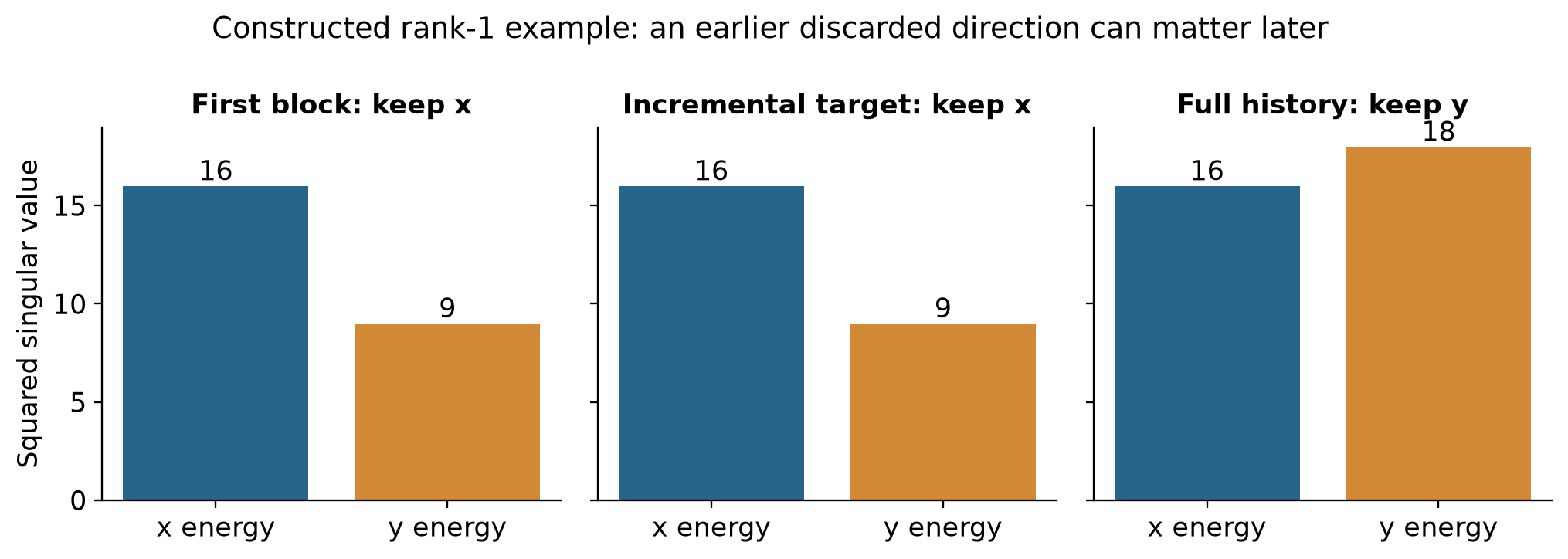
Figure 4. Constructed rank-1 example described above. The arriving row cannot recover the old discarded energy, so the incremental and full-history decompositions select different directions. Bars show squared singular values, not model measurements.

4.4 Reorthogonalization preserves the represented product

Repeated low-precision updates erode orthogonality. Write thin QR factorizations $U=Q_U R_U$ and $B=Q_B R_B$. Factor the small middle matrix without truncation:

$$R_U\Sigma R_B^\top=\widetilde U\widetilde\Sigma\widetilde B^\top. \tag{11}$$

Replacing the factors by $Q_U\widetilde U$, $\widetilde\Sigma$, and $Q_B\widetilde B$ leaves $U\Sigma B^\top$ unchanged in exact arithmetic. It restores a useful numerical coordinate system; it cannot reconstruct historical information already discarded by rank truncation.

The main configuration reorthogonalizes every 256 rows processed by regular folds. The initial value refit is excluded from that counter. Projection, residual work, core decomposition, reorthogonalization, and reconstruction use FP32, even when persistent factors use a two-byte format. A byte-count comparison must therefore separate persistent storage from transient arithmetic buffers.

5. Returning to attention: costs that the small core does not remove

Algorithm 3. Decode with separate K and V position sets

1. Store the new K and V rows exactly at the new position.
2. Advance each recent window; enqueue unprotected departing rows.
3. For V's first refit, wait for r_V pending rows and refactor
   the reconstructed old V history plus those rows.
4. Otherwise, fold the oldest b rows when a complete block exists.
5. Reorthogonalize after the configured number of regular folds.
6. Move folded positions into compressed-position lists.
7. Reconstruct K and V; scatter exact and approximate rows into
   their original token positions, independently for each path.
8. Restore head dimensions and apply each key's original RoPE.
9. Evaluate ordinary dense attention on the reconstructed cache.

For $X\in\{K,V\}$, let $n_X$ and $e_X$ count compressed and exact rows, and let $\beta_f,\beta_e$ be bytes per factor and exact scalar. The persistent per-layer payload is

$$M_{persist}=\beta_f\sum_X k_X(n_X+d+1) +\beta_e d\sum_X e_X. \tag{12}$$

The first term includes $U$, $B$, and the diagonal of $\Sigma$; the second includes protected, recent, and pending rows. There is no separately cached $\Sigma B^\top$ product in the reported configuration. Metadata, unused allocated capacity, reconstruction tensors, and workspace are outside this formula.

At equal rank and precision, with $n$ compressed rows and $e$ exact rows per path, dense storage is $2\beta(n+e)d$, while compressed storage is $2\beta[r(n+d+1)+ed]$. The persistent representation saves bytes only when

$$n(d-r)>r(d+1),\qquad n>\frac{r(d+1)}{d-r},\quad r<d. \tag{13}$$

The exact-row term cancels when comparing the same sequence, but its fraction still controls the achieved overall ratio. For $d=1024,r=128$, the break-even compressed-history length is just over 146 rows; the first integer is 147. This is an illustrative payload calculation, not a measured model-specific threshold.

With fixed exact overhead, the compression ratio approaches $d/r$ as history grows. Both dense and low-rank storage still grow linearly. The method reduces the slope from $O(nd)$ to $O(nr)$; it does not offer a fixed memory budget for arbitrarily long generation. Prompt protection can also grow with the diversity of the input and the union across heads.

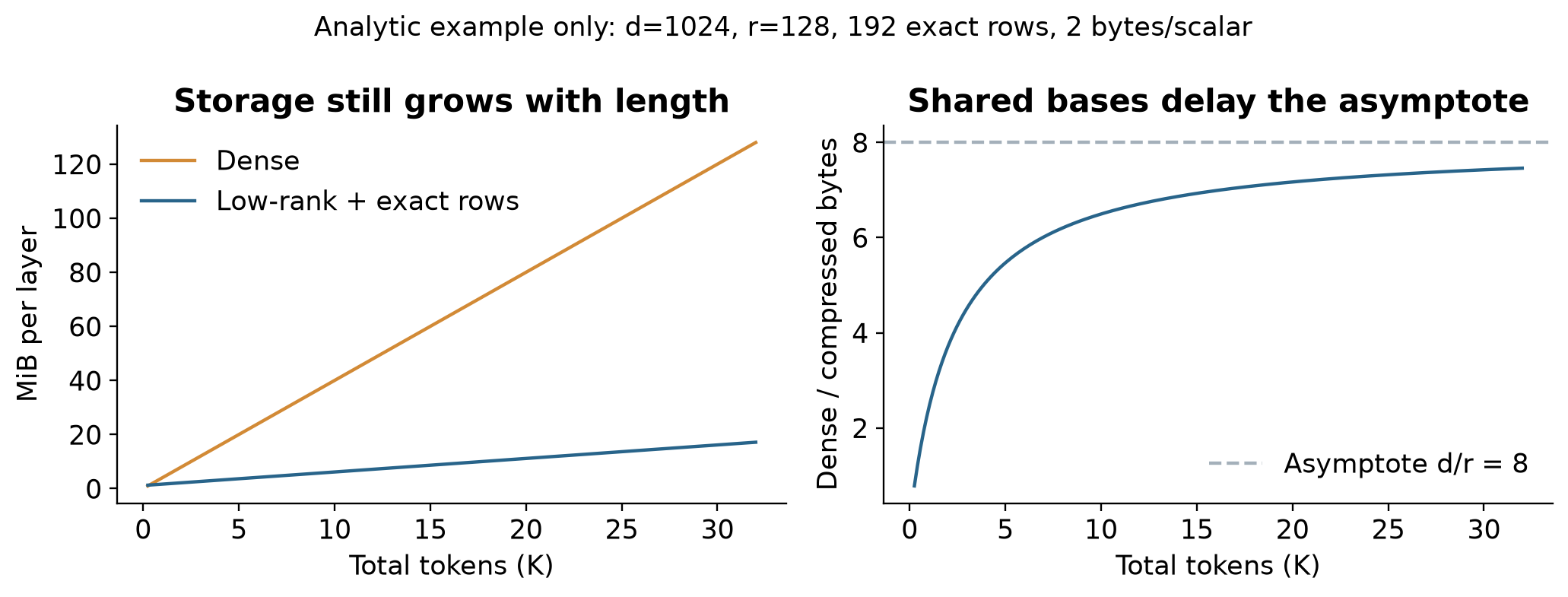
Figure 5. Analytic example from (12), with $d=1024$, $r=128$, 192 exact rows per path, and two bytes per scalar. It excludes metadata and workspaces. The 8× limit is an asymptote for these chosen parameters, not a paper benchmark.

Projection and residual calculation require $O(bdr)$ work. Residual construction factors a $d\times b$ matrix; the core has at most $r+b$ rows and columns. Updating historical coefficients costs $O(nr(r+b))$ per block. Dividing by $b$ amortizes that cost across arriving tokens but leaves an $n$ dependence. Reorthogonalization and reconstruction likewise involve the history.

A natural alternative is attention directly on factors. Without position-dependent rotations, scores from a reconstructed matrix could be reassociated, and values could be mixed in the reduced space. Pre-RoPE key storage complicates this route: each token has its own rotation. Applying one common rotation to a shared basis is generally not equivalent. A fused factor-aware kernel must preserve that positional computation and handle exact rows, differing K/V sets, and numerical precision. It is a promising research direction, not a delivered speedup in this paper.

6. Reasoning evidence at matched persistent memory

6.1 MATH-500: the strongest comparison

The main experiment uses all 500 questions, one sampled generation per question, temperature 0.6, top-p 0.95, top-k 50, and a 16,384-token total prompt-plus-generation limit. Original-model, iS-KV, and R-KV runs use paired questions, prompts, question-specific seeds, and an identical answer evaluator. Empty and non-finite outputs count as wrong. This controls several important sources of variation while leaving sampling variability across repeated runs unmeasured.

The table below transcribes iS-KV and matched R-KV points from paper Table 1. Compression is measured at the original model’s output lengths. The small differences between the methods’ byte footprints are retained in the original source; the displayed compression column here belongs to iS-KV.

Model	Rank	Compression	iS-KV accuracy	R-KV accuracy	Gain, pp
DeepSeek 8B	128	4.060×	82.6%	78.2%	4.4
DeepSeek 8B	96	4.811×	81.8%	76.4%	5.4
DeepSeek 8B	64	5.917×	78.2%	72.6%	5.6
Qwen3 8B	128	4.681×	92.0%	71.4%	20.6
Qwen3 8B	96	5.644×	89.2%	68.8%	20.4
Qwen3 8B	64	7.118×	87.8%	60.8%	27.0

The original-model accuracies are 83.6% and 94.4%. Reducing rank from 128 to 64 costs iS-KV 4.4 points on DeepSeek and 4.2 on Qwen. The large advantage over R-KV therefore coexists with a real approximation penalty relative to the original model. Retention is useful, but does not erase the quality–memory tradeoff.

The appendix reports paired question-bootstrap 95% intervals for the DeepSeek gains over R-KV: [1.6, 7.2], [2.0, 8.8], and [2.2, 9.0] percentage points. These support an advantage on that paired question sample. They do not cover a new model family, a different generation policy, or all sources of run-to-run variation. On Qwen at rank 96, the paper reports only 0.056% relative mismatch between the matched byte footprints.

Memory matching includes R-KV’s 128-token staging buffer and iS-KV’s factors and exact rows. Evaluating at original-model lengths prevents a method that stops earlier from receiving an artificial compression benefit. This is a good experimental choice: generation quality can change output length, so actual-run bytes alone would mix representation efficiency with stopping behavior.

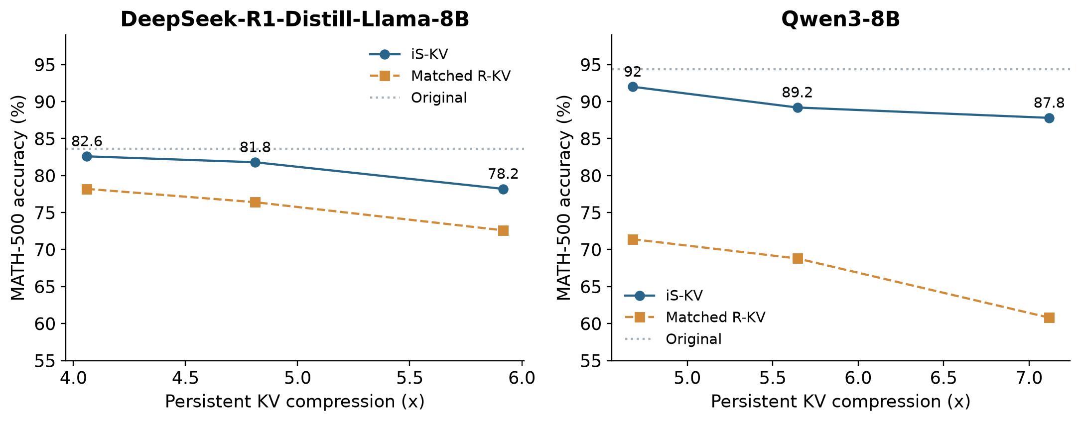
Figure 6. Redrawn from paper Table 1. R-KV is plotted at the corresponding iS-KV compression coordinates for visual comparison; the original table documents the slight byte mismatches. Each model has its own original baseline. No peak-memory or throughput claim is encoded here.

6.2 Baselines with weaker comparability

SnapKV is below iS-KV at all six reported points, but its results were retained from existing baseline summaries. Its reported percentages are not all multiples of 0.2%, as a single 500-question binary-outcome evaluation would require. The paper infers correct counts by rounding, rather than counting per-question outcomes. Accordingly, the paired R-KV comparison deserves more weight than a claim of equally controlled evidence against every baseline.

The released OjaKV setting reaches 62.0% on DeepSeek at roughly 1.30× compression, versus 83.6% for the original model. Attempts to target higher compression stopped after 30, 28, and 60 generations; all observed outputs repeated until the limit without EOS. These are 118 observed failures across three configurations, not a scored 500-question zero-accuracy result. The finding is informative about those settings, but cannot establish that every well-tuned online-basis alternative must fail.

6.3 AIME and component ablations

AIME 2024 and 2025 each contain 30 questions, with one sample per question and a 32,768-token total limit. Qwen3-8B uses BF16 factors here. On AIME 2024, increasing rank from 64 to 192 raises iS-KV accuracy from 43.3% to 76.7%, while matched R-KV rises from 13.3% to 43.3%. At rank 192, iS-KV and the original model both solve 23 questions. AIME 2025 at the same rank yields 56.7%, versus 40.0% for R-KV and 63.3% for the original model.

Each question changes accuracy by about 3.3 points. Equal aggregate counts do not prove identical solved questions or statistical equivalence. These results extend the qualitative advantage to longer reasoning, but precision, task size, and generation budget all differ from the main MATH experiment.

A fixed 80-question DeepSeek subset isolates components at rank 96. The original model solves 67, K-only solves 68, V-only solves 65, frozen bases solve 51, and fully adaptive iS-KV solves 65. The frozen-to-adaptive difference is 14 answers, or 17.5 points. That is stronger evidence for adaptation than the one-answer K-only gain is evidence for improving the original model.

K-only and V-only compress by 1.64×, while joint adaptive compression reaches 4.61×. They share per-path rank, not total memory. The equal 65-answer totals for V-only and joint compression do not prove keys are harmless: the error sets may differ, and the comparison is small. A memory-matched K/V rank-allocation study would answer a different, practically useful question.

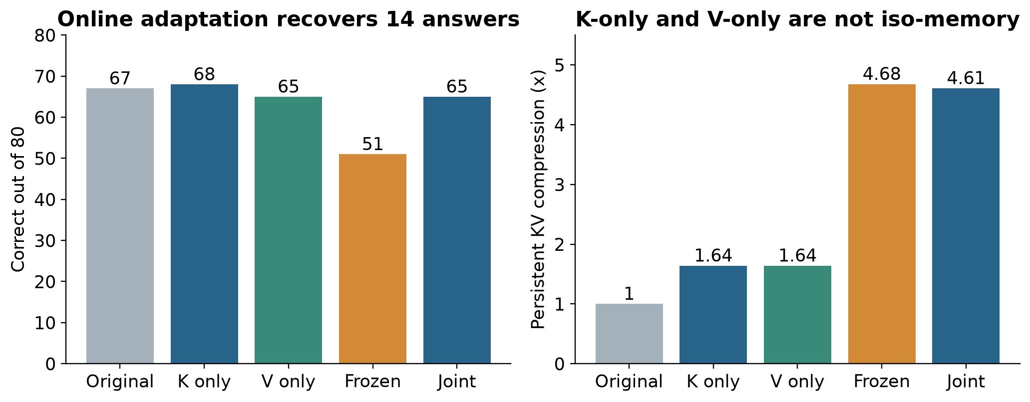
Figure 7. Redrawn from paper Table 3. Left: counted correct answers on 80 questions. Right: persistent compression ratios. Frozen and adaptive bases have similar total storage, whereas the single-path variants use substantially more memory.

7. Long prompts, numerical precision, and actual generation time

7.1 RULER exposes model and task dependence

The 64K RULER study uses 11 tasks and ten examples per task. Rank-160 configurations retain all three single-needle task scores of 100 for the tested models, but their mean scores still fall. GLM-4-9B-1M changes from 89.6 to 87.8 at 2.67× compression; Llama-3-8B-Instruct-Gradient-1048k changes from 87.3 to 86.3 at 2.29×; Llama-3.1-8B changes from 85.6 to 79.0 at 2.23×.

Rank 96 is more damaging on Llama-3.1-8B: its mean is 71.7, with multi-query retrieval 46.6 versus 100 and multi-value retrieval 41.6 versus 100. A headline single-needle success does not summarize more demanding retrieval. The small number of examples and task-specific metrics further limit fine-grained conclusions.

These are not pure rank ablations. Rank 96 uses 128-row recent windows and 16-row folds, while rank 160 uses different key-update settings and a 512-row recent value window. The better score can reflect both rank and the exact-storage policy. Future comparisons should hold these controls fixed or explicitly attribute the differences.

7.2 Persistent bytes go down while measured time goes up

The A40 efficiency test uses DeepSeek, batch size one, rank 128, synthetic 8K/16K/32K inputs, and exactly 1,024 greedy decode steps. It times prefill plus decoding, excluding loading, compilation, and inspection. Each point is one fresh-process run without inference warmup.

Input	Original time	iS-KV time	Overhead	Original KV	iS-KV KV
8K	38.83 s	47.45 s	22.2%	1.125 GiB	0.746 GiB
16K	49.04 s	58.32 s	18.9%	2.125 GiB	1.185 GiB
32K	68.63 s	74.70 s	8.8%	4.125 GiB	1.808 GiB

The reported persistent-KV savings rise from 33.7% to 56.2%. They exclude reconstructed caches and workspace, so the table does not establish that peak GPU memory falls by the same fraction. The timing direction is a slowdown at all three points. Its diminishing percentage is interesting, but a single unwarmed run per point cannot establish stable latency tails or a crossover at larger lengths.

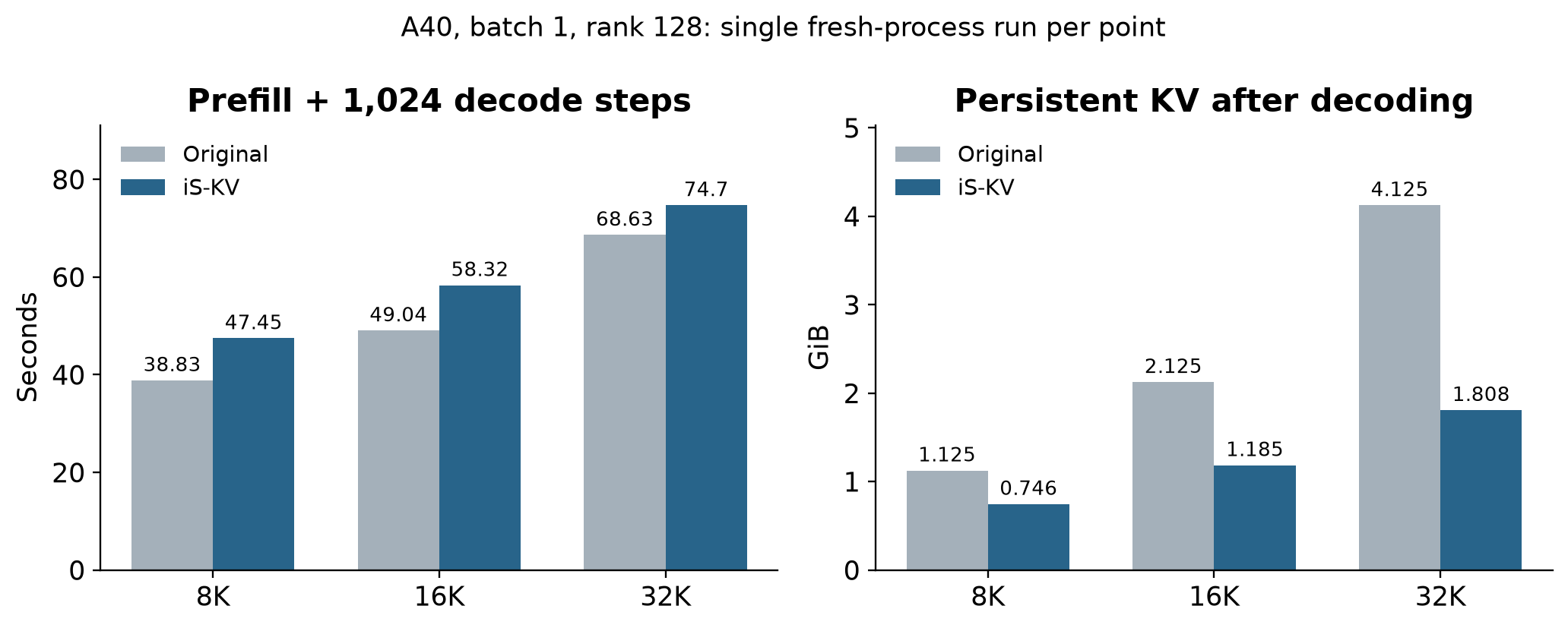
Figure 8. Redrawn from Section 4.4 and paper Fig. 4. The fixed-output protocol avoids comparing different generation lengths. The memory panel counts persistent KV payload, while the time panel includes updates and reconstruction.

7.3 Precision is part of the method configuration

The MATH runs store factors in FP16 and compute updates in FP32. At longer Qwen generations, the authors observe factor entries exceeding FP16’s largest finite value, 65,504, leading to infinities and NaN logits. Raw BF16 keys and values do not have the same dynamic-range limit. Derived factors, especially singular-value scales, need not have the same range as their input entries.

All 32K experiments therefore use BF16 factors. BF16 and FP16 both occupy two bytes, so this change preserves the nominal persistent-byte accounting. It does not preserve numerical results. BF16 has a wider exponent range and fewer mantissa bits. In a DeepSeek rank-128 AIME 2024 comparison, both formats reach 56.7% accuracy, yet mean generation length changes from 15,541 to 18,126 tokens and the share reaching the limit changes from 13% to 27%. An unchanged score can conceal substantially different behavior and cost.

The appendix’s factor-drift diagnostic is excess relative error over a fresh same-rank SVD of a reference matrix $X$:

$$\delta=\frac{\|\widehat X_{inc}-X\|_F}{\|X\|_F} -\frac{\|\widehat X_{fresh}-X\|_F}{\|X\|_F}. \tag{14}$$

It should be read separately from truncation error and the stale-coordinate probe. On one 8,192-step AIME trajectory, Table 5 reports key excess errors around 0.0016–0.0071 and value errors around 0.0160–0.0207 at ranks 96/128. Those small differences support the numerical fidelity of the maintained-factor update on that trajectory; they do not prove that the approximation to the original KV cache is equally small.

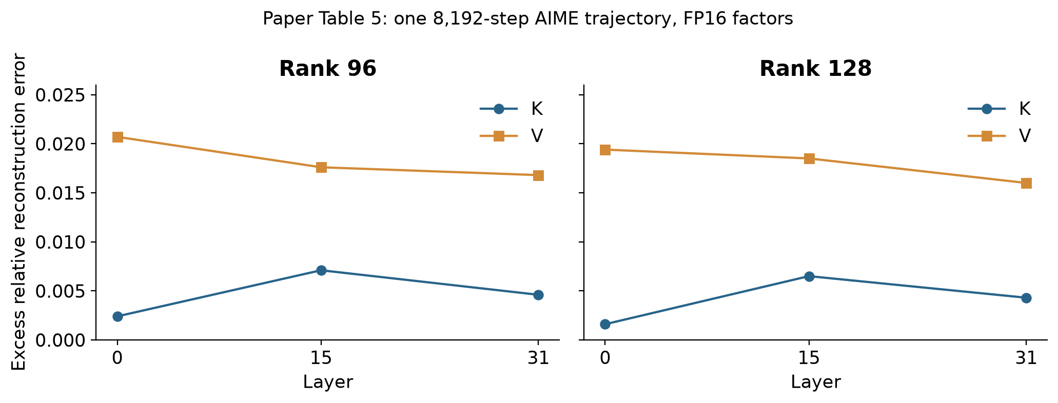
Figure 9. Redrawn from paper Table 5. These are excess relative reconstruction errors under (14) for one FP16 trajectory, not accuracy losses or uncertainty intervals. The worst displayed key value is 0.0071.

Reorthogonalization reduces the reported $\|U^\top U-I\|_F$ from $9.5\times10^{-3}$ to $1.1\times10^{-3}$ in one layer/rank setting, while the median relative product change is $2.4\times10^{-4}$. The appendix says this did not reduce reconstruction error within 8K steps. Its function is to maintain numerical conditions for continued updates, rather than to reverse information loss.

8. Reproduction priorities and design alternatives

An independent evaluation should first specify what is being held fixed. To reproduce the main comparison, use identical prompts, question seeds, evaluator, total-token limit, factor precision, and original-model reference lengths. Report counted answers, actual stopping lengths, persistent bytes, peak allocated memory, and peak reserved memory separately. These are proposed evaluation controls, not a report of tests run here.

The cache policy needs its own record: ranks for each path, protected chunk count and size, value dilation radius, recent-window sizes, regular fold sizes, first-value-refit behavior, residual tolerance, and reorthogonalization interval. The byte accounting should include the factor basis and singular values as well as per-token coordinates. Counting only $nr$ coefficients overstates savings at short lengths.

Several alternatives target different failure modes. Freezing a prompt basis avoids historical-coordinate rewrites, but the 80-question ablation shows a substantial cost for that choice. Increasing the exact window delays compression and may protect current local dependencies, but increases storage and does not recover older discarded directions. Lowering rank reduces the storage slope while increasing truncation error; increasing block size amortizes updates but retains more pending exact rows and enlarges the core.

A precision change is not just an implementation detail. FP32 storage may reduce numerical issues but costs more bytes; BF16 preserves two-byte storage while altering rounding and stopping. Per-layer or asymmetric K/V ranks could spend memory where reconstruction is more consequential. The current evidence that values are more sensitive makes that hypothesis reasonable, but neither a value-heavy allocation nor a query-weighted loss is established by this paper.

A useful diagnostic hierarchy starts with an algebraic product check for a single update, then tracks discarded residual energy and excess reconstruction error, then evaluates attention or logit perturbations on fixed continuations, and finally scores free generation. These levels answer different questions. A faithful SVD update can still approximate the wrong directions for reasoning, and a small teacher-forced error can compound during free generation. No single low-level number replaces the answer-level experiment.

9. Limitations

The central limitation is irreversibility at the feature level. Every token position survives, but discarded components do not. Successive locally optimal folds need not equal a fresh low-rank factorization of the original history. If future queries depend on previously weak directions, approximation can fail even though the token remains addressable.

The second limitation is resource accounting. Persistent KV payload is a useful quantity but is not peak HBM use. Dense reconstruction and FP32 work can overlap with the model’s other allocations. The current latency experiment demonstrates overhead, and there is no integrated serving throughput result. Fixed rank also leaves total storage and some update work growing with length.

The empirical coverage is narrower than a general inference guarantee: two 8B reasoning models, one generation per question, small AIME sets, an 80-question component subset, and ten examples per RULER task. Longer-context settings change factor precision or update policy. SnapKV summaries and early-stopped OjaKV settings have additional comparability limits.

Finally, the method uses a reconstruction surrogate and a largely uniform rank policy. Stable retained energy across depth is useful evidence, but it is not proof that all layers have the same task sensitivity. The appendix itself shows substantial variation in the rank required to retain 99% spectral energy, including a 122–338 range on Qwen. A fixed rank is an operational simplification, not a discovered law of model structure.

10. Critical analysis

10.1 Separate coordinate consistency from information preservation

The paper convincingly identifies a coordinate-consistency error: a changed basis with stale coordinates can corrupt already represented states. Correcting that error is necessary for a coherent online factorization. It is not sufficient for preserving the information that long reasoning will need. The token-revival motivation concerns future relevance, while the Frobenius objective concerns current aggregate energy. Those are connected heuristically, not by a task-aware theorem.

A stronger follow-up would measure which revived tokens suffer large attention-logit perturbations and whether those perturbations predict answer changes. Compare uniform rank with query-weighted or layer-adaptive allocation at identical persistent bytes. Such a study would test the missing link between spectral fidelity and future utility, instead of relying only on average singular-value decay.

10.2 The representation has a systems debt

The small-core argument can make the method look independent of history length. It is the decomposition dimensions that are bounded, not the complete update. Historical coefficients must be rewritten, and dense states must be reconstructed for the reported attention path. As $n$ grows, that memory traffic can dominate the elegant small SVD.

The most informative next systems experiment would profile time and peak memory separately for projection, core SVD, old-coordinate rewrite, reorthogonalization, reconstruction, and attention. It should use repeated warmed runs, several batches, and realistic output-length distributions. Only then can one choose between a factor-aware kernel, less frequent basis refreshes, or a policy that occasionally spends extra rank to reduce costly rewrites. These alternatives trade numerical fidelity, memory, and scheduling flexibility rather than providing a free optimization.

10.3 Prompt protection needs an explicit budget study

Unioning outlier chunks across heads and dilating protected values is a sensible safeguard, but its exact-row count can vary sharply with the prompt. This is why short reasoning prompts and 64K retrieval inputs should be analyzed separately. The reported compression ratio bundles low-rank quality with a protection policy that can keep different portions of different inputs exact.

A useful ablation would cap protected bytes, sweep the dilation radius, and show the resulting retrieval/answer Pareto curves. At the same total budget, compare spending an extra unit of memory on protected prompt rows, recent rows, value rank, or key rank. That would reveal whether the success is primarily due to adaptive factorization, conservative exact retention, or their interaction.

10.4 Comparisons should probe robust tuning, not only failure endpoints

The paired R-KV results are the most persuasive part of the experimental evidence. The OjaKV failures are worth reporting, but early stopping prevents an ordinary full-dataset comparison at those compression points. A carefully tuned alternative with a documented calibration budget would make the online-factorization claim stronger. Likewise, a fresh SnapKV run using the identical evaluator would remove the summary-count ambiguity.

For numerical stability, both factor formats should be evaluated on the same tasks, including stopping distributions and repeated seeds. The observed equality in one accuracy total alongside a large length shift is a warning against validating precision choices through accuracy alone. A system can preserve the score while changing latency, memory residency, and tail behavior.

11. Conclusion

iS-KV offers a clear way to reason about online KV compression: retain positions, compress old vectors, and update their coordinates whenever the shared basis changes. Block-incremental SVD makes the coordinated update mathematically tractable, while exact recent and protected states limit where approximation is applied.

Its evidence supports improved reasoning accuracy over the tested eviction baselines at matched persistent KV memory. It does not support losslessness, constant-memory generation, or an inference speedup in its current evaluated form. The next decisive step is to connect task-sensitive compression with a factor-aware execution path, while measuring complete memory use and generation behavior.

References

1. Zhao et al. iS-KV: Online Low-Rank KV Cache Compression via Block-Incremental SVD, v1, 2026-10-02. Main source: Sections 3–4, Tables 1–5, Appendices A–B.
2. Brand. Fast Low-Rank Modifications of the Thin Singular Value Decomposition, 2006. Classical update underlying the paper’s construction.
3. Bhatnagar et al. STAR-KV: Low-Rank KV Cache Compression via Soft Thresholding for Adaptive Rank Control, 2026. Related direction for adaptive rank allocation; not evaluated independently in this review.
4. Chen et al. KV-CoRE: Benchmarking Data-Dependent Low-Rank Compressibility of KV-Caches in LLMs, v2, 2026. Related analysis of data-dependent compressibility.