DictLLM: Shared Dictionaries for Post-Training Compression

Review date: 2026-11-13 (UTC)
Author: Zhongzhu Zhou
Paper reviewed: DictLLM: Post-training Compression of Large Language Model with Dictionary Kernels
Paper authors: Jinho Park, Se Young Chun, Mingoo Seok
arXiv: 2611.08082v1, 2026-11-05

What a shared dictionary buys

Two transformer blocks rarely implement the same function. They can nevertheless draw their linear projections from a related set of directions. DictLLM takes that distinction seriously: it shares the input-side basis of a projection across a small group of layers and leaves a separate coefficient matrix in each layer. It then prunes the coefficients, fits the basis again with the sparse coefficients frozen, and finally quantizes both factors. The main recipe uses calibration inputs and a pretrained model without gradient fine-tuning. Appendix A6 studies a separate variant that adds LoRA.

The useful comparison is between two ways of spending the same compression budget. A factorization alone must buy each extra basis direction together with a dense row of coefficients for every output. DictLLM can keep a larger shared basis and pay for only some of its coefficients. The paper measures improvements over several low-rank methods at matched reported projection budgets. It also reports a useful but more modest systems result: on the tested GPU with FP16, batch one and a sparse backend, decoding rises from 102.35 to 126.81 tokens/s. The roughly 5.1× representation gain highlighted in the abstract belongs to the NVFP4 quality comparison, a different measurement.

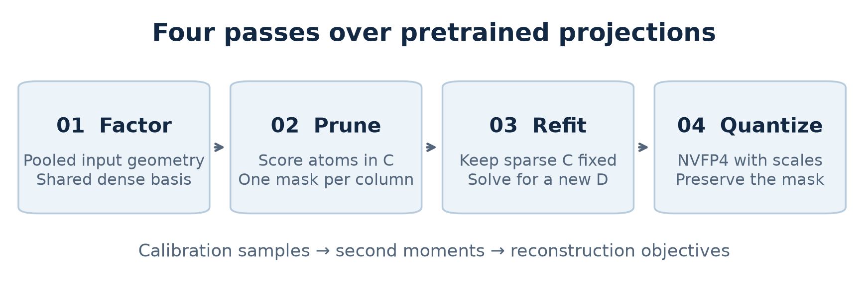
Figure 1. Original schematic based on paper Fig. 1 and Section 3. The refit sits between pruning and quantization because pruning changes which columns can use each atom.

I read v1 through Appendix A10. Numerical examples and arithmetic checks in this review use small matrices or values printed in the paper; I did not rerun compression or GPU benchmarks. The main question for the review is where the savings come from and what would have to remain true to get them on a different model, dataset or serving shape.

Prerequisites: projections, rank and calibration

Take a linear map with the paper’s orientation: rows of $X_\ell$ are tokens, $W_\ell$ is $d_{\rm in}\times d_{\rm out}$, and $Y_\ell=X_\ell W_\ell$. The group $g$ contains compatible weights of one projection type; for the equal-shape derivations below, both widths are common. Each column of the dense weight determines one output channel. In a factored projection each column becomes a linear combination of input-side vectors, which the paper calls atoms. Let $D_g$ have $k$ columns, and let $C_\ell$ have $k$ rows. The approximate forward pass is

$$W_\ell\approx D_gC_\ell,\qquad Z_\ell=X_\ell D_g,\qquad Y_\ell\approx Z_\ell C_\ell. \tag{1}$$

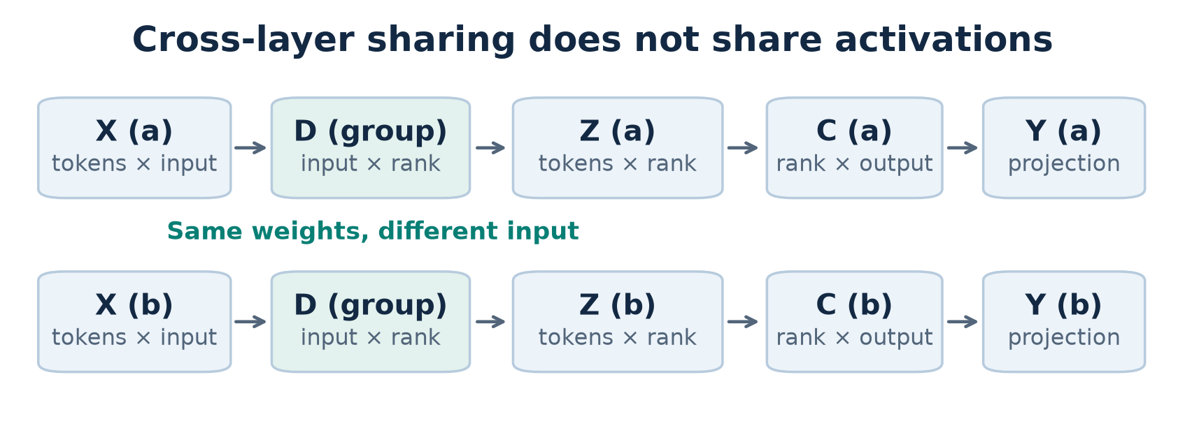
Figure 2. Original schematic based on paper Fig. 2. A dictionary can be loaded or cached for reuse if the runtime permits. The intermediate remains specific to the layer and its inputs.

Within this factorization there are two distinct constraints. Rank limits the dimension of the span that all reconstructed columns may occupy. Coefficient sparsity limits the number of atoms a given column can use inside that span. The active subset can vary from column to column. For example, one output can use atoms 1 and 3 and another can use 2 and 4. A coefficient count below the number of entries of a lower-rank dense factor does not imply that the resulting matrix has lower rank. Nor does sparsity in $C_\ell$ usually imply sparsity in the product $D_gC_\ell$.

Think of calibration as measuring the cost of moving a weight in different input directions. If a column error is $r$ then the observed error across sampled tokens is $X_\ell r$. Its energy equals $r^\top S_\ell r$, where $S_\ell=X_\ell^\top X_\ell$. The word covariance here refers to a Gram matrix or uncentered second moment; no centering is needed to obtain this identity. Correlations matter. If the calibration inputs all look like $(a,a)$, errors pointing along $(1,-1)$ can be invisible, while equal-sized errors pointing along $(1,1)$ are amplified. Centering would remove the contribution of the mean to this reconstruction metric. A scalar mean over tokens would not record which pairs of channels move together.

SVD writes a matrix as a sum of orthogonal rank-one terms, each weighted by a singular value. Under the ordinary squared Frobenius norm, keeping the $k$ largest singular values minimizes error over all rank-$k$ matrices. The discarded squared singular values add up to that error. For calibration-aware compression the Frobenius argument applies to the transformed weight. It says how well the group reproduces its action on a chosen input distribution; it does not say that a particular direction is dispensable to a rare task.

For inference, I track three separate budgets. A retained-value budget counts elements that must be represented. A byte budget also counts bit widths, scales, masks, padding, fixed embeddings and output heads. A time budget includes reads, arithmetic, intermediate writes, sparse indexing and launch overhead. A method can make excellent progress on the first two and yield a small or negative improvement on the third. The paper’s tables provide examples of why those units should not be mixed.

The budget: trading shared rank against sparsity

For $n$ equal-shaped projections, the original group has $n d_{\rm in}d_{\rm out}$ values. After factorization the dictionary costs $d_{\rm in}k$ once, and each layer contributes $kd_{\rm out}$ coefficients. At retained density $1-p$ the ideal count and fractional saving become

$$\begin{aligned} N_0 &= n d_{\rm in}d_{\rm out},\\ N_p &= d_{\rm in}k + n(1-p)kd_{\rm out},\\ \rho &= 1-N_p/N_0,\qquad G=N_0/N_p. \end{aligned} \tag{2}$$

Here $\rho$ is a fraction removed and $G$ is a multiplicative gain. Set $p=0$ and rearrange $\rho_{\rm fac}=1-k(d_{\rm in}+nd_{\rm out})/(n d_{\rm in}d_{\rm out})$ to choose rank. In practice rank is an integer and may need hardware alignment; round down if the value budget is binding.

$$k=\left\lfloor\frac{(1-\rho_{\rm fac})n d_{\rm in}d_{\rm out}}{d_{\rm in}+nd_{\rm out}}\right\rfloor. \tag{3}$$

At a 20% factorization reduction and width 4096, a private square factor has rank 1638, a dictionary shared by two has rank 2184. The private down projection in Appendix A1.2 is $11008\times4096$, giving 2388. Ignoring rounding, the two-layer square group pays one third of its factored values for $D$, two thirds for $C$. With $p=0.194$ its retained fraction becomes $0.8(1-2p/3)\approx0.6965$. This is about 30.35% removed, consistent with the paper’s Q/K/V figure up to rounding. Other projections can have different fractions even with the same $p$ and $\rho_{\rm fac}$, so the whole-model setting comes from a weighted sum of matrix counts.

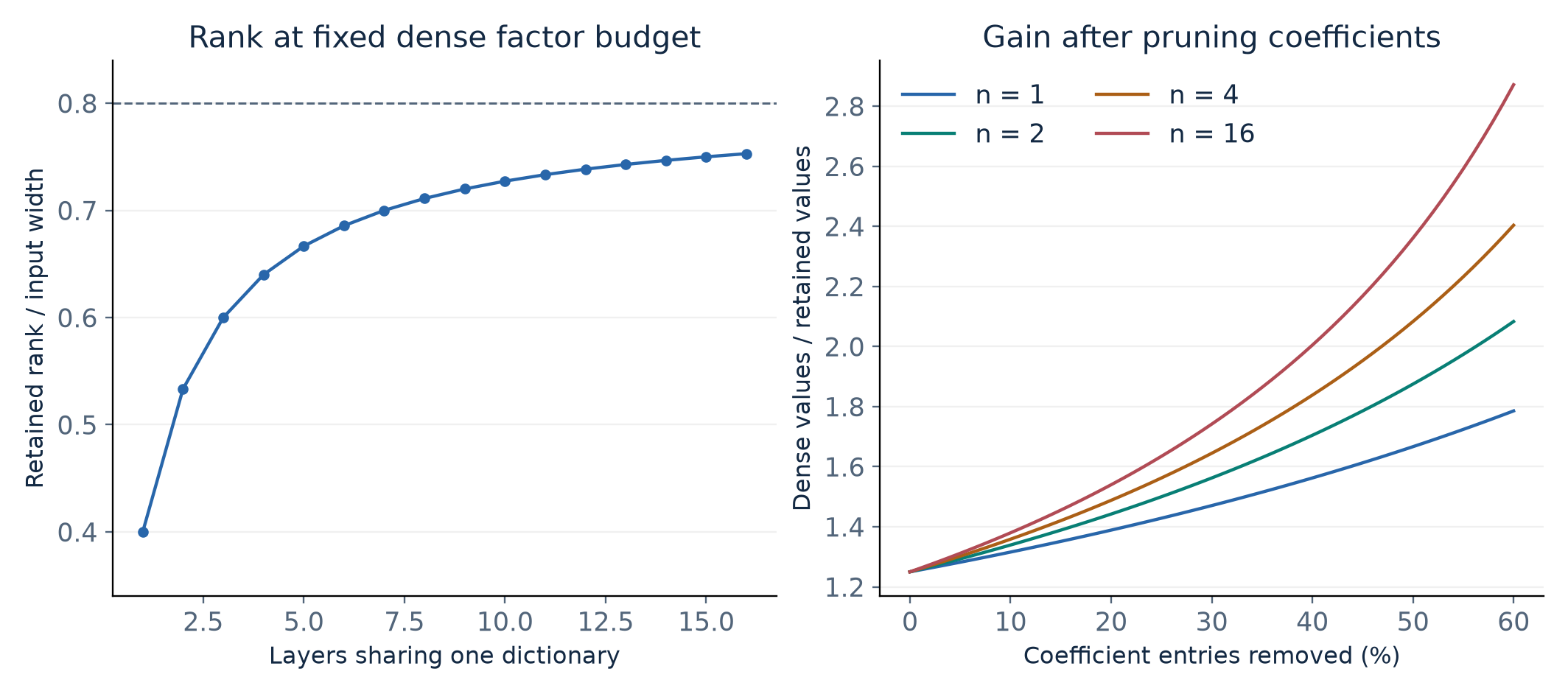
Figure 3. Original curves from equations (2) and (3), equal square matrices, 20% factorization reduction, ideal nonzero counts. Larger groups buy more rank per stored value but do not guarantee a better shared subspace.

The arithmetic suggests making every group as large as possible. That is a bad default. With square matrices and fixed $\rho_{\rm fac}$, the rank fraction approaches $1-\rho_{\rm fac}$ as $n$ grows, giving diminishing returns. More importantly, the union of the directions used by all layers can expand faster than the rank allowance. If two equally weighted layers each need a different one-dimensional direction, one shared atom loses some signal regardless of how well coefficients are selected. Output and down projections are normally private in the paper. Appendix A6 enlarges groups to 4, 8 and 16, shares those projections too, uses 60% coefficient sparsity at fixed ranks, and adds LoRA to all projections. Reported gains of 2.9×, 3.5× and 3.9× accompany perplexities 10.26, 12.32 and 15.89. The increasing storage gain comes with an increasing quality cost even with adaptation.

The linear contribution of sparsity to equation (2) also has a ceiling. Even if every coefficient could be erased at no loss, the dense dictionary remains. In the two-layer square example it is about 26.67% of the original group count. In a very wide input and narrow output projection, the dictionary can dominate the budget much sooner. This is one reason I would tune ranks by projection shape and measured error rather than expect one uniform sparsity number to be optimal.

Method I: a tractable activation-aware SVD

The group objective in Section 3.2 penalizes the residual of each layer in its own input metric. If $R_\ell=W_\ell-D_gC_\ell$, the per-layer objective and the surrogate used for initialization can be written side by side. Let $W_g$ and $C_g$ denote the horizontal stacks and $S_g=\sum_\ell S_\ell$.

$$\begin{aligned} \mathcal L_{\rm layer} &=\sum_{\ell\in g}\operatorname{tr}(R_\ell^\top S_\ell R_\ell),\\ \mathcal L_{\rm pool} &=\|S_g^{1/2}(W_g-D_g C_g)\|_F^2 =\sum_{\ell\in g}\operatorname{tr}(R_\ell^\top S_g R_\ell). \end{aligned} \tag{4}$$

The second line uses the same input metric on every group’s output column. It adds cross-layer terms $\operatorname{tr}(R_\ell^\top S_jR_\ell)$ for $j\ne\ell$. If all $S_\ell$ are equal, the losses differ by a constant scale. If they are merely proportional, the pooled loss still applies equal weights to the blocks, while the original objective gives more weight to layers with larger multipliers. When the second moments point in different directions, there is no reason for the optima to coincide. Pooling buys one SVD and one coefficient curvature proxy per group; it trades away a guarantee for the original objective.

Assume $S_g$ is positive definite for the derivation. Set $A=S_g^{1/2}W_g$ and $B=S_g^{1/2}D_g$. Since the transformation is invertible, minimizing $\|A-BC_g\|_F^2$ is equivalent to choosing any rank-at-most-$k$ approximation to $A$. Write the truncated SVD of $A$ as $U_k\Sigma_k V_k^\top$. The paper places the singular values on the dictionary side and splits $V_k^\top$ by layer.

$$D_g=S_g^{-1/2}U_k\Sigma_k,\qquad C_g=V_k^\top,\qquad \mathcal L_{\rm pool}^{\star}=\sum_{j>k}\sigma_j(A)^2. \tag{5}$$

If one uses a Cholesky factor $S_g=LL^\top$, the transform multiplying $W_g$ on the left is $L^\top$, not $L$. Inverting the transform can be implemented as a linear solve. An exactly singular Gram matrix assigns zero cost to its null space. A supported-space pseudoinverse or positive damping resolves the algebra in different ways; damping also changes the metric by charging for movement in low-coverage directions. Appendix A2 reports $10^{-4}$ damping for covariance and Hessian operations unless otherwise specified. If one uses the damped metric for factorization and the undamped metric for scoring, identities that presume the same metric should not be treated as exact.

An elementary example shows why the transform matters. For $S=\operatorname{diag}(4,1)$ and $W=\operatorname{diag}(1,1.5)$, raw SVD retains the second direction at rank one. The error scored under $S$ is $4\cdot 1^2=4$. In the transformed weight the diagonal is $(2,1.5)$, so the first direction is retained and the squared error is $1.5^2=2.25$. I checked the two residuals with a direct matrix calculation. This is an illustration, not a result on a transformer. On a held-out distribution where the two channels reverse their relative importance, the same choice can reverse its advantage.

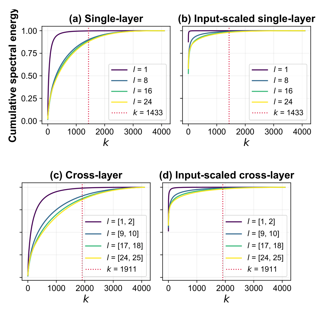
Figure 4 (paper Fig. A1). Cropped panels from v1, p. 19. Read panel labels: (a) and (c) are raw; (b) and (d) are input-scaled. Curves concentrate sooner with scaling; the dashed ranks compare equal factorization reduction.

Appendix A5 also separates K, V, gate and up projections from private output and down projections. The early query layer in Fig. A1 concentrates energy faster than several deeper layers. A spectrum is a diagnostic of average reconstruction under a metric, not a cross-layer similarity measure on its own: two weights can both have sharply concentrated spectra in different subspaces. To justify pairing them, I would measure the per-layer held-out residual after a shared fit at the proposed rank and compare with independently fitted layers at the same byte cost.

The factorization differs from strict weight tying, where $C_\ell$ would also be fixed across the group. It differs from classical $k$-SVD in Appendix A1.1, where sparse codes and dictionary atoms are alternated, often for an overcomplete dictionary. DictLLM uses an undercomplete basis with a rank set by compression and does a single post-prune update for scalability. In the single-query projection test of Fig. 3, dense input-scaled SVD has 0.071% relative activation error, pruning raises it to 0.163%, and refitting lowers it to 0.125%; the tested $k$-SVD gives 0.132%. That test can motivate a fast initialization; it cannot establish model-wide quality at equal packed size.

Method II: prune in coefficient space

With $D_g$ fixed, a perturbation of one coefficient column $c$ by $\delta$ changes the projection weight column by $D_g\delta$. The squared activation change is therefore a quadratic in the coefficient coordinates. Expand the norm for one layer, then pool its metric to obtain the practical proxy of Appendix A1.3:

$$\begin{aligned} \|X_\ell D_g\delta\|_2^2 &=\delta^\top D_g^\top X_\ell^\top X_\ell D_g\delta,\\ H_\ell &=D_g^\top S_\ell D_g,\qquad H_g=\sum_{\ell\in g}H_\ell=D_g^\top S_gD_g . \end{aligned} \tag{6}$$

The mathematical Hessian of the squared norm is $2H_\ell$; the paper uses the Gram matrix as its curvature proxy. The factor of two has no effect on the undamped minimizer. The loss is for a perturbation relative to the unpruned factorized projection. If the factorized projection already has a nonzero dense-target residual, the change in the dense-target error includes a cross term with that residual. The perturbation-only loss omits it. That is reasonable as a way to preserve a fitted function; it cannot guarantee monotone improvement relative to the original dense weights. The refit addresses some of this residual after the mask is chosen.

For a single deletion of row $i$, constrain $e_i^\top\delta=-c_i$, where $e_i$ is a coordinate unit vector. Let $K=H_g+\lambda I$ be positive definite and $P=K^{-1}$. The Lagrangian for $\frac12\delta^\top K\delta$ has derivative $K\delta+\mu e_i=0$. Hence $\delta=-\mu P e_i$. Substituting into the constraint gives $\mu=c_i/P_{ii}$; inserting the solution in the squared loss gives the saliency used in the paper:

$$\delta_i^\star=-\frac{c_i}{P_{ii}}P e_i,\qquad s_i=(\delta_i^\star)^\top K\delta_i^\star =\frac{c_i^2}{P_{ii}}. \tag{7}$$

The index $i$ on $\delta_i^\star$ labels the coordinate being removed; the expression is a full vector. If $K$ is diagonal, deleting a value changes only that coordinate and the score is $K_{ii}c_i^2$. If the inverse has off-diagonal entries, the perturbation adjusts other rows. This explains why pure magnitude ranking ignores both direction sensitivity and compensation. It also explains the cost difference relative to a weight-space curvature factor: the inverse is $k\times k$ instead of $d_{\rm in}\times d_{\rm in}$, shared across columns. This is a reduction of the inversion dimension, not a statement that the rest of the compressor scales only as $k^3$.

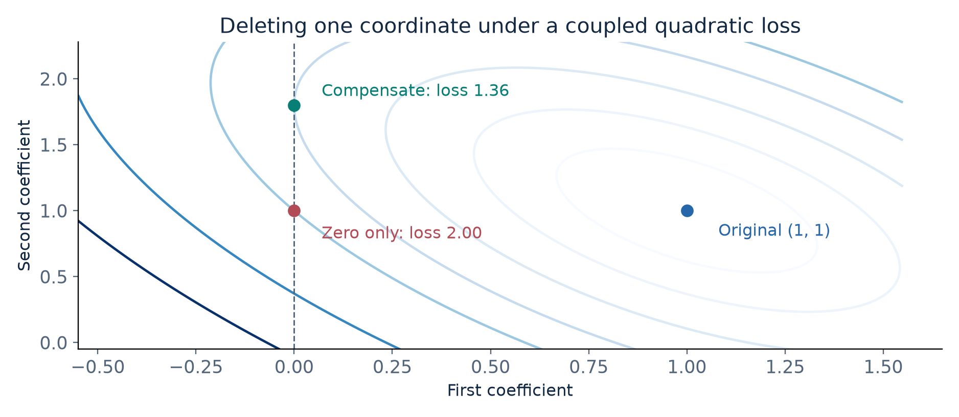
Figure 5. Original calculation using diagonal entries 2 and 1 and off-diagonal 0.8. Along the zero-first-coefficient line, moving the second coefficient from 1 to 1.8 reduces loss from 2 to 1.36.

There is an instructive nuance here. In the ideal Step 1 algebra with the very same $S_g$ and exact whitening, $D_g^\top S_gD_g=\Sigma_k^2$. Then $P$ is diagonal even with isotropic damping added in coefficient space. The pooled pruning score becomes a singular-value-weighted magnitude rule. It can still outperform raw magnitude, since the factors put scale into $D$. But any claimed gain specifically from cross-coordinate compensation needs a setting that breaks this diagonal identity, for instance using a per-layer metric, using a different metric from the whitening one, or using the refitted dictionary. The reported ablations compare full method choices. They do not identify which of these mechanisms generates the margin. The coupled two-coordinate drawing explains the general quadratic update and is not an illustration of an exact freshly whitened pooled dictionary.

Algorithm 1 — Fixed-inverse pruning within a coefficient block

The following is a reading of paper Algorithm 2. Each column has its own ordering. Scores are calculated at the start of the block; the compensation uses the current coefficient when the row is reached. A final mask enforces the chosen support even if earlier coordinates were perturbed again.

1. Form P from inverse(transpose(D) S D + damping I); read its diagonal.
2. Partition the output columns into blocks of size at most B.
3. For each column in a block, sort rows by c[i]^2 / P[i,i].
4. Mark the first floor(p*k) rows in that column's order.
5. For each marked row i in that order, read its current c[i].
6.     Subtract P[:,i] * c[i] / P[i,i] from the column.
7. Set every marked entry exactly to zero and keep the mask.

The exact joint solution for deleting a set $J$ replaces the scalar denominator with a small matrix. With $E_J$ the matrix of selected coordinate vectors, enforce $E_J^\top\delta=-c_J$. Solving the stationarity equations as above gives

$$\delta_J^\star=-PE_J(E_J^\top PE_J)^{-1}c_J,\qquad s_J=c_J^\top(E_J^\top PE_J)^{-1}c_J . \tag{8}$$

If the selected rows interact, a rank-one move for a later deletion can move an earlier deleted value away from zero. The final mask reasserts feasibility but need not restore the minimum of the joint quadratic. Recomputing the inverse on surviving coordinates or solving once for the final support are alternative approaches. Even an exact solve for a proposed support does not solve the combinatorial problem of choosing that support. The paper’s Table 3 reports the same rounded WikiText-2 PPL, 9.89, for its lazy method and full inversion in one setting. This is evidence about the quality/cost trade at that setting, not equality of their masks or outputs.

Method III: refit the dictionary and quantize the factors

Let $\widetilde C$ be the concatenation of the pruned coefficients; its values and zeros stay fixed. With a common positive definite left metric, the least-squares gradient of $\|S_g^{1/2}(W_g-D\widetilde C)\|_F^2$ is $2S_g(D\widetilde C-W_g)\widetilde C^\top$. Setting it to zero cancels $S_g$ and gives an ordinary right-side normal equation. If $\widetilde C\widetilde C^\top$ is singular, damping the right factor corresponds to penalizing the metric-weighted dictionary norm $\|S_g^{1/2}D\|_F^2$, or equivalently doing ridge regression in transformed coordinates:

$$D_{\rm refit}(\widetilde C\widetilde C^\top+\lambda I) = W_g\widetilde C^\top. \tag{9}$$

An ordinary unweighted ridge penalty added to a weighted residual instead gives $S_g(D\widetilde C\widetilde C^\top-W_g\widetilde C^\top)+\lambda D=0$. These two regularizers coincide only in special cases. The closed-form update reported in Section 3.3 is consistent with the common-metric interpretation or unweighted ridge on $W_g$. Using the original layer-specific metrics gives

$$\sum_{\ell\in g}S_\ell D\widetilde C_\ell\widetilde C_\ell^\top =\sum_{\ell\in g}S_\ell W_\ell\widetilde C_\ell^\top \tag{10}$$

for an undamped stationary point. Now no single left factor cancels, in general. This derivation distinguishes what the closed form optimizes from the initial statement of the objective. It also suggests a way to improve the approximation without changing deployment shape: solve the per-layer normal equation iteratively as a linear operator on $D$, using the pooled update as a starting point.

For a small fixed-support example, use $W=((3,1,2),(1,2,1))$, with tuples denoting rows, and $\widetilde C=((1,0,1),(0,2,0))$. The original dictionary is $I$. The coefficient Gram is $\operatorname{diag}(2,4)$ and $W\widetilde C^\top=((5,2),(2,4))$. The zero-damping update gives columns $(2.5,1)$ and $(0.5,1)$. The second output becomes exact. The first and third outputs each err by 0.5 in their first entry. Direct multiplication gives squared error 0.5 instead of 8 with $I$. Nothing has been added to the support. An atom that has no active coefficient anywhere instead leaves a zero Gram row and an unconstrained direction in the unregularized fit. Small damping keeps the solve defined; it does not make the atom useful.

Algorithm 2 — Group compression and export

This outline follows paper Algorithm 1. The quantization proxy for the codes is the dictionary-induced metric. Algorithm 1 passes the pre-refit proxy into the quantization call; rebuilding the proxy using the deployed dictionary is a distinct testable alternative.

1. Collect per-layer input Gram matrices from the dense model.
2. For each projection type and group, pool the Gram matrices.
3.     Derive rank k from the factorization budget.
4.     Factor the input-scaled concatenation; split codes by layer.
5.     Compute coefficient curvature using the shared dictionary.
6.     Apply Algorithm 1 of this review to each code matrix.
7.     Freeze the sparse codes and solve the dictionary refit.
8.     Quantize the refitted dictionary using input curvature.
9.     Quantize the codes using their curvature; preserve zeros.
10.    Export dictionary, per-layer codes, scales and support.

The last two operations introduce different kinds of error. For $\widehat D=D+\Delta D$ and $\widehat C=C+\Delta C$, subtracting $DC$ gives

$$X(\widehat D\widehat C-DC) =X\Delta D C+XD\Delta C+X\Delta D\Delta C. \tag{11}$$

With $C$ held fixed, the Gram of $X$ describes the input side of dictionary error, but the true output loss also depends on the right-side $CC^\top$. With $D$ held fixed, the Gram of $XD$ describes the left metric of the codes. Joint quantization has a cross term and correlated changes to both factors. The paper’s factor-specific scheme is a manageable approximation. It uses NVFP4 block scales and a masked error-compensating quantization step for $C$. Appendix A2 gives a relative Hessian damping factor of 0.1 for masked quantization. I would treat recalculating $D^\top S_gD$ after refit or quantization as an ablation, not assume it is used in the reported table.

What the quality comparisons establish

The authors calibrate on 256 WikiText-2 sequences of length 2048, collecting statistics from the original model. They evaluate language modeling on WikiText-2, PTB and C4 and use seven zero-shot tasks in LM-Evaluation-Harness. Appendix A2 specifies the raw accuracy field, not its length-normalized variant, and describes the PTB text join. WikiText-2 PPL is the exponential of average token negative log likelihood. A reduction in PPL is easier to compare across settings if translated back to the underlying log loss. Between 19.99 and 10.59, for example, the log difference is $\log(19.99/10.59)\approx0.635$ nats per token on the same benchmark. It is not a 9.4-point increase in accuracy.

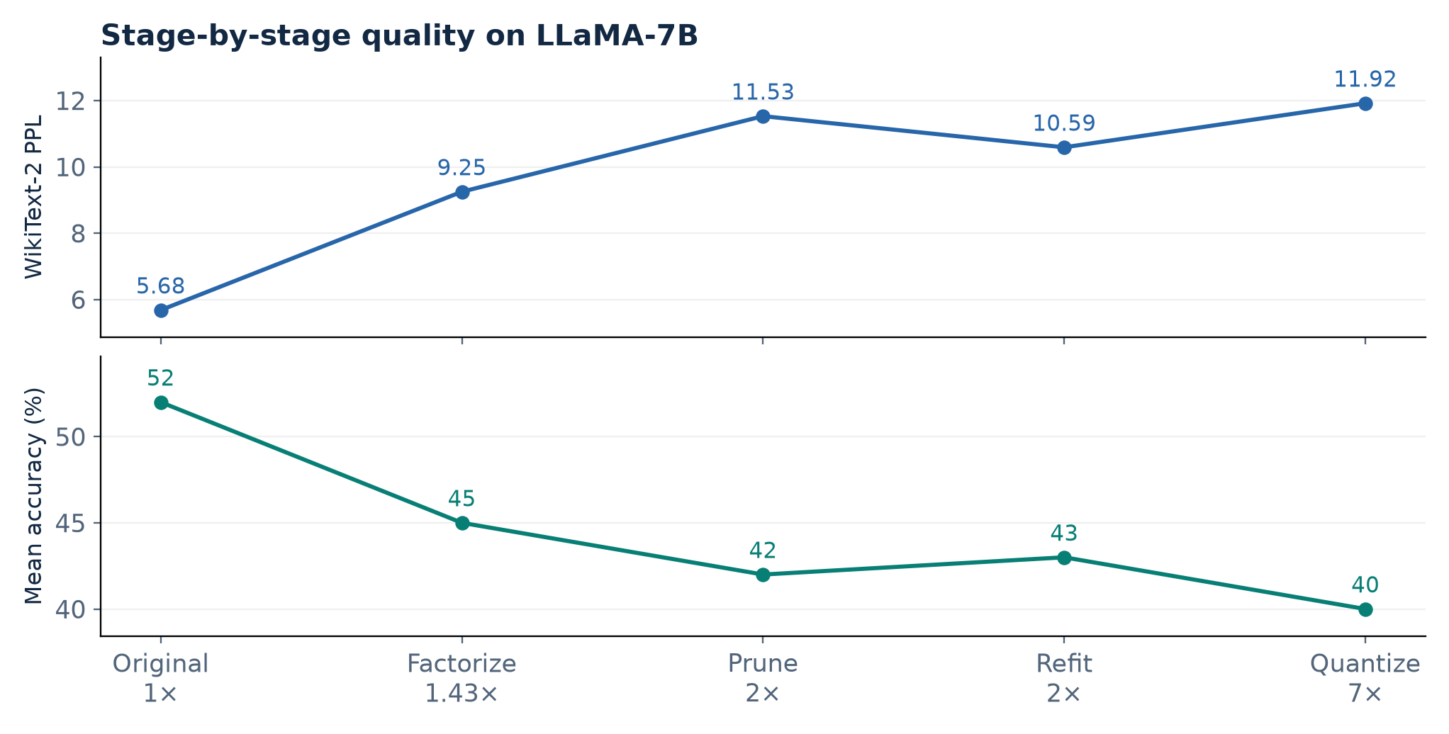
Figure 6. Redrawn from paper Table A7. Only the prune-to-refit comparison holds reported size fixed. The accuracy panel uses the rounded seven-task means in that table.

At 2× in Table 1, the unquantized DictLLM point gives 10.59, 35.67 and 29.12 PPL on WikiText-2, PTB and C4. Basis Sharing gives 19.99, 126.35 and 88.44, respectively. Relative to the dense model’s 5.68, 8.35 and 7.34, there is still substantial damage. This is a better compression frontier within the reported family, not quality preservation at arbitrary gain. The observed WikiText-2 gap to Basis Sharing widens as compression is pushed harder; this should not be extrapolated beyond the measured budgets. ASVD shows particularly large degradation at high compression here, making Basis Sharing the more informative comparison.

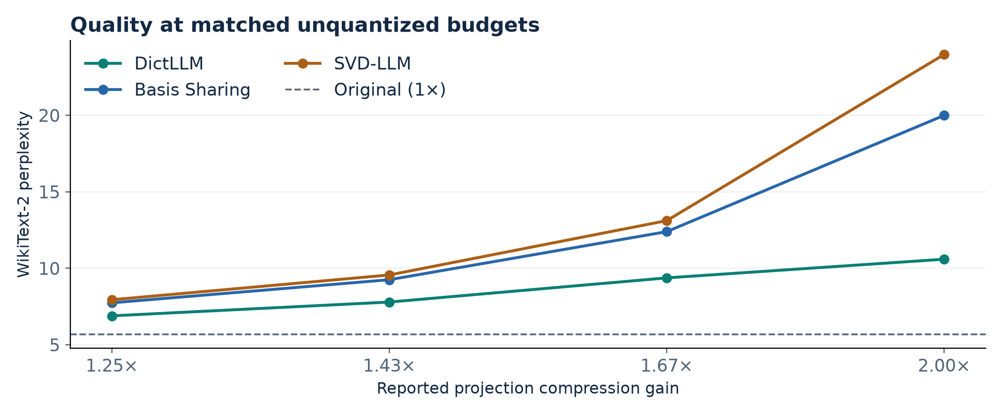
Figure 7. Redrawn from paper Table 1. The dashed line is the dense original. The horizontal axis enumerates tested budgets; the connecting lines guide the eye.

Appendix A4 provides a useful fixed-size comparison. At 2×, refitting moves WikiText-2 PPL from 11.53 to 10.59 and C4 from 33.82 to 29.12. The seven-task average moves from 0.42 to 0.43 in the rounded table. Figure 5 shows a larger benefit from refitting at higher sparsity in its separate 20% factorization sweep, 1.04 PPL at 50% sparsity versus 0.06 at 20%. This is what one would expect if deleting more coefficients makes the old dense-factor dictionary a worse match to the surviving support. It does not imply that refitting an aggressively pruned model can recover the original behavior. Table 2 further indicates that pruning only $C$ does better than pruning $D$ or splitting the pruning between them at a matched 1.43× gain. Dense-to-dense in that table uses more factorization to reach the same budget, so compare quality under budget, not only the presence of zeros.

There is evidence beyond the base model. Table 5 tests 1.25× on LLaMA2-7B, OPT-6.7B and Mistral-7B; DictLLM gives 6.93, 11.36 and 6.46 WikiText-2 PPL, respectively, ahead of each reported low-rank baseline there. Appendix A3 covers Qwen3-1.7B, 8B and 14B; at 1.43× the average accuracy margins over Basis Sharing are 2.67, 5.27 and 3.65 percentage points. The 8B sweep at 2× shows 16.58 versus 29.61 WikiText-2 PPL and 41.63% versus 34.31% mean accuracy. Even so, the 1.7B original is 54.05% and its 1.43× DictLLM is 39.37%, so a method winning the compressed comparison need not be a good deployment choice for that base model. The appendix is evidence for more than one architecture and size, with no corresponding NVFP4 throughput sweep across these models.

Appendix A7 makes the comparison more useful by adding pure pruning, pure quantization and combinations. At the reported 5× point, DictLLM FP4 gets 8.48 WikiText-2 PPL versus 11.38 for Basis Sharing plus 4-bit AWQ and 13.99 for Basis Sharing plus 4-bit GPTQ. The pruning-only comparison at 80.32% sparsity is especially severe for SparseGPT and Wanda. At roughly 7×, the paper reports 40.39% mean accuracy for DictLLM versus 32.00% for GPTQ and 30.07% for AWQ, both run at two bits. These are useful near-budget comparisons among specific pipelines. They do not match precisions, layouts, runtime backends or tuning search, and they do not isolate the effect of sharing. Appendix A13’s unquantized magnitude comparison is closer, but still changes pruning and refit jointly. I would also keep Table 1’s 0.52 dense average distinct from A9–A13’s 53.94% dense average; the unrounded task values in the latter do not merely give more digits for all Table 1 entries.

Table 6 shows partial recovery from LoRA on query and value projections using rank 8 and scale 4. At 2× the paper reports DictLLM PPL 8.71 in this run. Appendix A2 says that experiment omitted dictionary refitting, so the difference from the 10.59 main row does not isolate adding LoRA to the main refitted recipe. Figure 6’s 32-to-256 calibration sweep also omits refit. Table A8 in Appendix A6 instead varies quantization calibration: 16 sequences give 9.06, 128 give 8.88 at about eight times the cost. That is a separate axis from the samples used to fit the original dictionary. Data diversity, sequence length and calibration token count can interact even at the same sample count.

From retained values to measured decoding

A 4-bit weight takes half a byte if perfectly packed. NVFP4 uses a shared 8-bit scale per block of sixteen values in the standard block format. Ignoring outer scales, padding, masks and alignment, the value plus scale costs 4.5 bits per value, so the gain against the same FP16 value array is $16/4.5\approx3.56$. This agrees with the all-NVFP4 gain in Table 4, whose denominator is the already factorized and pruned FP16 model. With a reported 1.43× retained-value gain, multiplying by 3.56 gives approximately 5.09×, consistent with Appendix A2’s 5.08× before rounding. The 2× configuration gives about 7.12× under the same accounting. An embedding, scale array or sparse index only contributes to this multiplication if its treatment is included in the accounting.

Dictionary / coefficients	Gain vs factored FP16	WikiText-2 PPL
FP16 / FP16	1.00×	12.98
NVFP4 / FP16	1.61×	13.66
NVFP4 / FP8	2.60×	14.71
NVFP4 / INT8	2.60×	16.05
NVFP4 / NVFP4	3.56×	16.82

The table above transcribes the settings and metrics of paper Table 4. Its starting model uses 30% factorization reduction and 50% coefficient sparsity, so it is not the abstract’s 5.1× point. At the same 2.60× reported gain, FP8 codes beat INT8 codes by 1.34 PPL points here. The dictionary-only move from FP16 to FP4 costs 0.68 PPL, while moving on to FP4 codes costs another 3.16. This favors a mixed precision option if the target tolerates a higher byte count but values quality. It does not prove an inherent precision requirement for coefficient matrices: the effects depend on atom scaling, group layouts and the quantizer.

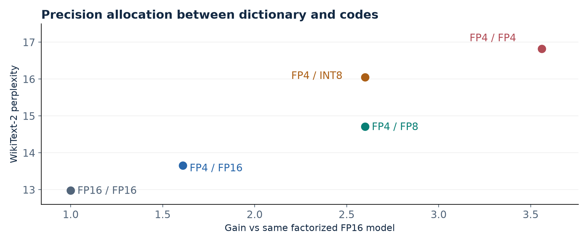
Figure 8. Redrawn from paper Table 4, which uses the same factorized FP16 model as the denominator for all gains. Labels list dictionary precision first.

A useful break-even calculation follows from the format. Consider $M$ logical coefficient entries. A dense array at effective bit width $b$ costs $Mb$ bits. A sparse array retaining fraction $q=1-p$ with $a$ extra bits per retained position and $h$ overhead bits per original position costs $M[q(b+a)+h]$ bits in a simplified model. It saves bytes precisely when

$$q(b+a)+h < b,\qquad p > \frac{a+h}{b+a}. \tag{12}$$

With $b=4.5$, $a=8$ and $h=0$, the threshold is 64% sparsity; 19.4% will not help this particular index format. A bitmap at one bit per logical position instead has $a=0,h=1$, so the simple threshold is 22.2%. Neither example represents the paper’s backend. They show why bit-packed masks, formats with constrained support, or ignoring some zeros in memory can change the winner. A bitmap also needs a fast way to map bits to data and preserve the order expected by the math kernel. Compression that improves the value ledger may still create an awkward storage layout.

Table A14 is the end-to-end evidence within a defined slice. All three configurations use FP16 on one RTX PRO 6000 Blackwell Max-Q, batch one, 128 prompt tokens and 100 autoregressive decode steps; there are ten measured runs after three warm-ups. The timer excludes prefill. DictLLM uses MACKO for sparse coefficients. From the table I calculate 126.81/102.35 = 1.239× versus dense, 126.81/113.59 = 1.116× versus Basis Sharing, 13.48/7.82 = 1.724× less weight memory as a ratio of sizes, and 13.66/8.02 = 1.703× for peak memory. The corresponding weight and peak reductions are about 42.0% and 41.3%. These are measured configuration differences. The ratio between the ideal 2× projection value budget and the realized weight-memory ratio is expected to depend on uncompressed parts and sparse overhead; the table does not assign a measured number of bytes to each cause.

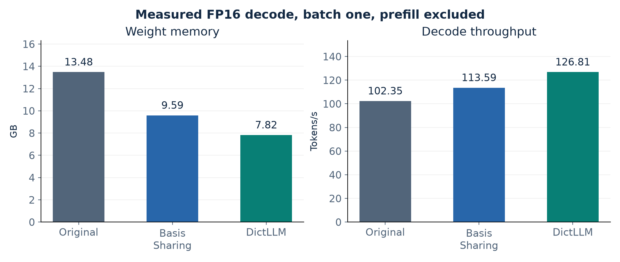
Figure 9. Redrawn from paper Table A14. These measurements are distinct from the FP4 quality and size points, and exclude prompt processing.

A two-pass projection needs an intermediate with $k$ features. Per group, ignoring biases, dense decode uses $n d_{\rm in}d_{\rm out}$ multiply-adds per token; ideal sparse factorized decode uses $nk[d_{\rm in}+(1-p)d_{\rm out}]$. The dictionary appears once in the value ledger but every participating layer must apply it. This is easiest to see for the 4096-wide two-layer example with $k=2184$ and $p=0.194$: the approximate ideal multiply-add fraction is $(2184/4096)(2-0.194)\approx0.963$, far larger than the retained-value fraction of about 0.697. Ignoring rounding and assuming the sparse kernel only visits retained values, this is roughly a 4% reduction in multiply-adds for roughly a 30% reduction in represented values. At larger batch or prefill the speed benefit can therefore narrow. A runtime might keep a dictionary in cache across adjacent layers, or read it again after intervening operations evict it. Neither is implied by the algebra. A fused path can avoid spilling some intermediate work, whereas a generic pair of matmuls and an irregular gather may cost more than the dense baseline. In attention-heavy workloads with long context, KV reads and non-projection work can dominate regardless of this weight savings.

Limitations and evidence boundaries

The hardware limit in Appendix A10 is the irregular sparsity of the coefficient factors. An unstructured sparse path can work when the runtime uses appropriate kernels, as the FP16 run shows, but a device that supports only certain block patterns or dense quantized products might not obtain the same result. There is no measured NVFP4 sparse end-to-end throughput or mobile energy comparison in v1. The LLaMA-7B decode test is narrowly scoped; batch one, prompt length 128 and a timer that excludes prefill do not characterize throughput under continuous batching or time to first token. A compressor intended for mobile deployment also needs compatibility with the actual device precision, memory hierarchy and supported operators.

The dataset limit matters even with all the model-family results. The initial dense activation Gram matrices come from short samples of one corpus. Calibration tokens may underrepresent code, long conversations, non-English inputs and rare attention patterns. A train-time token sequence also does not capture how the compressed model’s own generated errors alter later inputs. Weight-space or activation-space residuals are easier to measure than long-horizon task failures. Averaging seven multiple-choice scores can hide individual regressions, and those scores do not speak directly to tool use or instruction following. The table differences report point estimates; without per-example or across-seed uncertainty I would avoid strong claims about small margins.

There are two apparent presentation discrepancies in the source worth keeping separate from method interpretation. Figure 3 prints 13.07 s for $k$-SVD and 2.90 s for the proposed stages. Their ratio is about 4.51; nearby prose says 3.4× faster, with no alternate timing breakdown identified in the text. I retain the chart values and do not combine them with the prose multiplier. Figure A1’s caption reverses the with/without wording relative to the panel headers; the panels themselves mark (b) and (d) as input-scaled. Those readings do not alter the main perplexity or decode tables. In contrast, Table 3’s timing arithmetic, $13.49\times60/55.6\approx14.56$, is consistent with its 14.6× lazy-versus-full claim. This timing describes pruning, not inference.

Critical analysis: what I would change or measure next

Choose groups by the cost of a common metric

Grouping adjacent layers is cheap and gives a useful prior, but the relevant quantity is how much activation-weighted error pooling adds at a fixed footprint. Consider two layers with $S_1=\operatorname{diag}(9,9)$ and $S_2=\operatorname{diag}(1,1)$; let their scalar-output weights be $(1,0)^\top$ and $(0,2)^\top$. Compare rank-one dictionaries equal to the first or second coordinate, with the surviving coefficient fitted in each layer. Per-layer scores favor the first coordinate (4 versus 9); pooled scores favor the second (40 versus 10). The pooled choice upweights error on the second layer’s discarded direction using samples from the first. This final example only compares the two coordinate choices; it demonstrates a ranking reversal without claiming the exact optimizer over all possible directions.

Rather than use the pooled residual alone for grouping, I would predict each group’s cost from held-out per-layer residuals after a common fit. In addition to averaging them, report the worst layer and tail of the per-token residual distribution. Choose groups and ranks under a joint packed byte budget, retaining some private dictionaries where sharing forces a large trade. A simple experiment compares adjacent pairs, disjoint pairs selected by held-out cost, and private factors at the same budget. Keep coefficient sparsity pattern, precision and calibration sample count fixed in the first pass. This tests whether benefit comes from actual subspace overlap or from the additional rank amortization.

Separate score weighting, support choice and compensation

The whitening identity suggests a clean sequence of controls. First compare unweighted magnitude with $\Sigma_k^2$-weighted magnitude at the same fixed dictionary, same sparsity and no refit. Then compare pooled and per-layer metrics before refit, including their relative off-diagonal norm. Then hold a mask fixed and compare simply zeroing, the fixed-inverse update and an exact solve for surviving coefficients. Finally run the refit in each setting and compare whether it shrinks the quality gaps. The answers will say whether to spend memory on per-layer curvature or solve the main problem by scaling coefficients before ranking. They would also help explain why the full-inversion timing is so different in Table 3 even though rounded perplexity matches.

A subtle intervention is a change of basis inside the same dense subspace. For any invertible $A$ of size $k$, $(DA)(A^{-1}C)=DC$. For diagonal $A$ with nonzero entries, the zero pattern is unchanged. In the ideal undamped quadratic, single-coordinate deletion loss is invariant to that rescaling: the inverse diagonal and $c_i^2$ both scale by the reciprocal square of the atom scaling. Real damping and block quantization do not have that invariance. An orthogonal rotation preserves the dense product but can substantially change which individual coefficients are sparse. A deployment-oriented extension could optimize a constrained rotation and diagonal rescaling for both support and NVFP4 block range. It should be compared to the same unrotated dense product to avoid crediting it for a different initialization. Excessive rescaling can create outliers in the other factor, so choose balance using held-out activation loss rather than factor norms alone.

Let the accelerator constrain the support

Starting from arbitrary supports and packing them later can produce masks poorly matched to the target hardware. For a device with a fast structured sparse path, constrain support during the pruning decision and follow with the same dictionary refit. This will usually lose some flexibility compared with arbitrary masks. It can still win at the serving level if index overhead falls, address patterns improve and the sparse kernel avoids dense work. Compare equal packed bytes, then equal quality. Include the dense low-bit baseline with a native kernel, an unstructured sparse FP16 baseline, and the proposed structured format. If the target supports neither packed sparse low bit nor efficient fused projections, a dense mixed-precision factorization is an important control.

A useful first counterfactual is to hold quality and packing fixed while toggling whether $D$ is retained in fast memory across group members. Measure dictionary cache hits and intermediate write bytes together with wall time; this identifies whether a smaller file leads to reuse or just to a different read pattern. Break down query/key/value, output and MLP projections rather than average away a slow shape. Then run a short and long prompt sweep with batch 1, 8 and a saturated point. A gain on isolated decode with a short prompt can coexist with worse end-to-end latency when prefill dominates. Compare latency distributions and tokens per joule only if the experiment actually meters energy at the device or system boundary it claims.

Reproduction plan and readout

A reproduction should start with a small mathematical unit. For a real projection collect held-out activations, verify that raw versus input-scaled rank selection changes the intended residual, then compare the dense and factored forward equations at a rank high enough to approximate the metric’s numerical span. For a selected coefficient column, measure both the perturbation objective and the residual against the original dense projection. Log the damping, rank and condition numbers, as well as the mask before and after quantization. At this stage the smallest meaningful success is a refit that lowers held-out activation loss at unchanged count; if it does not, investigate Gram mismatch and overfitting before sweeping the entire model.

For the model experiment fix the exact model revision, tokenizer, evaluation split and token-window protocol. Match the Table A1 factorization and sparsity settings. Keep the dense reference for both benchmark series if their protocols differ, report raw and normalized task scores under explicit labels, and give uncertainty for small differences. Record per-stage wall-clock time separately from generation. Store one count for compressed projection nonzeros, one for all serialized bytes including support, scales and untouched weights, and one for peak process or device memory. For runtime publish the prompt length, actual generated length, backend, precision and warm-up; run prefill and decode measurements separately. This setup can test the reported quality and performance without assuming that a shape or format transfers automatically.

The small checks in this review evaluated equation (5) on a diagonal example, equation (7) on a coupled two-coordinate quadratic, the normal equation (9) on a fixed support, and ratios computed from the printed numbers. These are algebra and arithmetic checks. No checkpoint was re-compressed, no training was run, and no new hardware result is reported here.

Conclusion

DictLLM makes a practical case for spending some compression budget on a shared subspace and using sparsity and precision to control what is paid for inside it. The dictionary refit is the most persuasive isolated contribution: it improves quality at unchanged coefficient support and rank. The broader quality tables show advantages over several alternative compression pipelines, at the budgets and checkpoints measured. The study also demonstrates that at least one sparse FP16 runtime turns part of the storage savings into a decode gain. The open deployment question is what persists when the packed layout, calibration distribution and serving shape change together. I would prototype the shared refit first, then let measured bytes and target-kernel performance choose the sparsity and precision regime.

References

• Park, Chun and Seok. DictLLM, arXiv:2611.08082v1. Primary source; numbered tables, figures and appendices cited above. Author project page.
• Wang et al. SVD-LLM, and Wang et al. Basis Sharing. Two relevant low-rank comparisons; see references [8] and [9] of the source paper.
• Frantar and Alistarh. SparseGPT. Reference [14] in the paper, for the local quadratic approach to pruning.
• NVIDIA Blackwell Architecture technical brief. Reference [16] in the paper, for the block-scaled floating-point context.