Only Accepted Tokens Count: The Energy Cost of Speculation

Review date: 2026-11-12 (UTC)
Author: Zhongzhu Zhou
Paper reviewed: Only Accepted Tokens Count: An Energy Accounting of Speculative Decoding Under Latency Targets
Paper authors: Bole Ma, Ayesha Afzal, Jan Eitzinger, Harald Koestler, Gerhard Wellein
arXiv: 2610.40287v1, 2026-10-29

What the energy comparison measures

A drafter proposes the next few tokens. The target can verify those positions together and reuse weights within the pass. Reuse helps if enough of the proposed prefix survives. It is possible to serve the user faster while consuming more energy per output token, because the wider verification step draws more power or performs enough additional work to offset its lower number of steps.

Ma and colleagues compare five drafting schemes across eleven models and four attention families. The study uses SGLang with CUDA graph capture enabled for its principal serving measurements. The paper pairs each speculative setting with the same target, GPU, batch, task and serving settings without speculation. It also compares alternative batch sizes when it asks how a deployment should meet a latency target. I use those two comparisons for different questions. The first measures what the drafter changed at fixed concurrency. The second asks which configuration a service would actually choose.

The largest energy saving per model at batch one has a median of 54% across models in Table 2. At batch 64, the best measured scheme for every model that ran there saves 15–52%. That latter result is a best-of-schemes comparison. Several individual schemes have already crossed into an energy penalty. The strongest mechanism test uses Qwen3-4B on two GPUs. H200 supplies substantially more bandwidth with roughly the same measured BF16 arithmetic rate as H100. This lowers the arithmetic intensity at which verification becomes compute-limited. The same proposal width can run out of energy headroom at a smaller batch on H200.

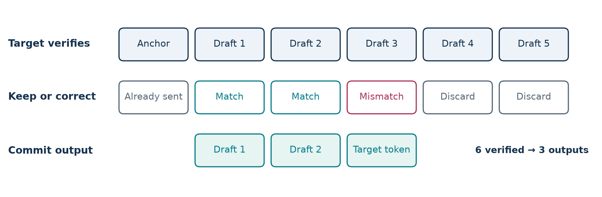
Figure 1. Original schematic based on Sections 2–3. The anchor and all five proposal positions occupy the verifier. The committed advance consists of two matching drafts and one target token in the example.

Prerequisites and notation

Decode, batching and the verification shape

Prefill consumes the input prompt and establishes cache and recurrent state. Decode extends each sequence one token at a time. In a small ordinary decode batch, a dense linear projection may read a large weight matrix to multiply by a single activation row per request. Batching combines independent rows in one matrix multiplication. It reduces duplicated weight reads per output token. A user still advances by one token per step. If the step time rises with batch, that user’s stream slows despite higher aggregate throughput.

Speculation adds rows from multiple positions of each request. Let $B$ be the actual concurrent request count, $k$ the number of drafted positions and $v=k+1$ the paper’s verified width including the opening token. The paper labels schemes by $v$. A DFlash-16 configuration has fifteen proposed positions. In the batched experiments the target verification shape carries $Bv$ positions regardless of how many drafts each request keeps. Acceptance is ragged inside that rectangular shape.

A head such as EAGLE3 or the MTP configurations in the paper generates positions successively. A block drafter such as DFlash or DSpark predicts a block in one pass. SGLang’s n-gram baseline in this study looks for a continuation on the host and uses no neural draft pass on the GPU. These are different sources of proposal cost. A vendor-trained assistant can be post-hoc. Gemma’s assistant is served through the MTP path but was trained after its target, unlike the co-trained heads of the Qwen3.6 and GLM examples.

Accepted draft tokens and committed output

Let $A$ be the count of consecutive draft tokens accepted before the first mismatch. In a full greedy round away from the output cap, the committed advance is $G=1+A$. The one is the target token at the mismatch or the extra target token after an entirely accepted draft. The opening token included in the verification shape was already emitted in an earlier round. A terminal round may be truncated and must use the actual count. In the accounting below I use $A$ for draft-only counts and $G$ for progress. When discussing the paper’s acceptance plots, I keep their reported accepted-length values as published. In particular, the plotted accepted length starts around one and is used as the advance statistic. I do not add an additional token to published values.

A greedy verifier accepts the longest prefix equal to the target’s greedy path. Each verifier row for a later draft assumes the earlier drafts. After a mismatch, predictions conditioned on that rejected prefix cannot safely advance the sequence. To see why the output matches the ordinary greedy path in ideal arithmetic, assume equality through the previous committed prefix. The first accepted draft equals the ordinary next token by the check. For each subsequent accepted draft the inputs also match, so the inductive step repeats. At the mismatch the target supplies the ordinary token. At full acceptance the target supplies the next token on the same prefix. Kernel-dependent roundoff and tie-breaking can perturb exact greedy equality in a real system. A probabilistic verifier has additional rejection and correction rules, so the following algorithm describes only the setting measured by this paper.

Algorithm 1. Greedy verification and state selection

1. Record the committed prefix and the cache or recurrent state at its boundary.
2. For each live request, obtain up to k proposed continuations.
3. Evaluate the anchor and draft positions causally in one target pass.
4. In draft order, compare each proposal with the greedy target prediction.
5. Stop at the first mismatch. Keep the matching draft prefix.
6. Append the target correction, or the extra target token if all matched.
7. Discard suffix KV entries or select the recurrent checkpoint at the boundary.
8. Track the correction as the next input where the engine uses an anchor.
9. Record actual committed output, verified width and any terminal truncation.

The loop is an explanatory reconstruction from Sections 2, 3 and 6. A recurrent update absorbs input into a state. A simple attention KV cache can often invalidate suffix slots, but a recurrent state already updated with a rejected token generally cannot undo that update. The paper describes keeping per-position states and selecting the one consistent with the accepted prefix. Conceptually, a corrected token still needs its own state advance at the appropriate input boundary. Mixing up a token’s emission with the processing of its input is a common source of an off-by-one error in this calculation.

From survival probabilities to useful work

For each proposal position $j$, define $S_j=\Pr(A\ge j)$, the probability that the prefix survives through position $j$. Express the random count as a sum of indicators and take expectations.

$$\begin{aligned} A &= \sum_{j=1}^{k}\mathbf{1}\{A\ge j\},\\ \mathbb E[G] &= 1+\mathbb E[A] =1+\sum_{j=1}^{k} S_j . \end{aligned} \tag{1}$$

Write $p_j=\Pr(A\ge j\mid A\ge j-1)$ when the conditioning event has positive probability. Multiplying conditional probabilities gives $S_j=\prod_{i=1}^{j}p_i$. This identity requires no independence assumption. For a toy constant $p<1$, the finite geometric sum gives

$$\begin{aligned} (1-p)\sum_{j=0}^{k} p^j &= 1-p^{k+1},\\ \mathbb E[G] &= \frac{1-p^{k+1}}{1-p}. \end{aligned} \tag{2}$$

At $p=1$ the limit is $k+1$. With $p=0.7$, six drafts yield about 3.06 expected output tokens and fifteen yield about 3.32. Nine extra verifier positions buy about 0.26 additional outputs per round in this example. Constant conditional acceptance is only a teaching model. In a real trace, the survival curve can steepen abruptly across difficult spans or vary by request. Its shape, particularly the tail beyond the current draft length, is relevant to the width decision.

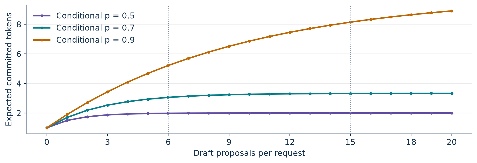
Figure 2. Original geometric illustration using Equation (2). Curves are analytic examples. A small increment in output can still be worthwhile when verification can absorb the extra positions at little cost.

Deriving the energy ledger

Energy per output token is a ratio of totals

Let $J_t$ be measured GPU-board energy in a matched observation window, and $G_{it}$ the number of output tokens committed for request $i$ in round $t$. A cumulative meter reading $M(\tau)$ yields the energy difference at the window boundaries. Write the measured metric as

$$e_{\mathrm{out}} =\frac{M(\tau_1)-M(\tau_0)} {\sum_{t}\sum_{i=1}^{B_t}G_{it}}. \tag{3}$$

Here $B_t$ can vary. If the experiment uses a fixed active batch and many comparable steps, let $\bar J_s$ be average energy per speculative step and $\bar G$ average committed advance per request per step. The same estimator can then be written $\bar J_s/(B\bar G)$. In ordinary decoding $\bar G=1$ and the corresponding metric is $\bar J_0/B$. Divide one by the other at the same $B$.

$$\frac{e_s}{e_0} = \frac{\bar J_s}{\bar J_0\bar G}, \qquad \bar G > \frac{\bar J_s}{\bar J_0} \quad\Longleftrightarrow\quad e_s<e_0 . \tag{4}$$

This derivation uses an equal active batch and matching measurement windows. It does not require $J_t$ and output length to be independent. Averaging per-round ratios would assign too much weight to short advances. The observed counter is over the whole generation window. The paper uses a decode accounting and flags a JoyAI latency exception where prefill was not subtracted. A system that compares per-request end-to-end energy must define its own prefill and idle boundaries.

Compare draft widths $k$ and $k+1$ under the same traffic mixture and batch. Let $J_k$ be the corresponding mean round energy and $G_k$ mean useful advance. In the special case that changing width preserves the distribution of the first $k$ predictions, $G_{k+1}=G_k+S_{k+1}$. Multiply the positive denominators of the two energy ratios to obtain a marginal test.

$$\begin{aligned} \frac{J_k+\Delta J}{G_k+S_{k+1}} &<\frac{J_k}{G_k},\\ \Delta J\,G_k &< J_k S_{k+1},\\ \frac{\Delta J}{J_k}&<\frac{S_{k+1}}{G_k}. \end{aligned} \tag{5}$$

The right side is the fractional extra useful advance. The left side is the fractional cost of the wider round. With $p=0.7$ and $k=6$, $S_7=0.08235$ and $G_6=3.0588$. The seventh proposal pays only if it adds less than about 2.69% to round energy. If changing a fixed-block drafter also changes its weights or its early predictions, estimate the full $\Delta G$ empirically. The original DFlash-7 and DFlash-16 comparison has exactly this confound. Width is a mechanism and the model checkpoints also differ.

Faster with a higher energy bill

Let $T_s$ and $T_0$ be mean durations per round and $\bar P_s$, $\bar P_0$ the corresponding average board power. Under the same simplification, the latency speedup $U$ is $T_0\bar G/T_s$. Substitute $J=\bar P T$ in Equation (4).

$$\begin{aligned} U &= \frac{\bar G T_0}{T_s},\\ \frac{e_s}{e_0} &= \frac{\bar P_s T_s}{\bar P_0 T_0\bar G} = \frac{\bar P_s/\bar P_0}{U}. \end{aligned} \tag{6}$$

A 1.20-fold gain in tokens per second with a 1.35-fold increase in mean power gives a 1.125-fold energy cost per token. These are illustrative values. Faster completion alone cannot determine energy. At equal observation scope the identity applies even if power fluctuates, because each mean power is total energy divided by its duration.

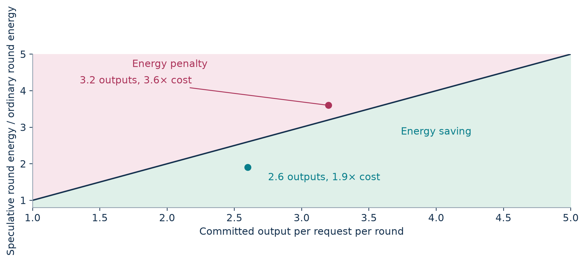
Figure 3. Original plot of Equation (4). The diagonal gives equal energy per token. The two marked configurations are illustrative, with a greater accepted advance still yielding a penalty if verification energy grows faster.

The hardware mechanism

Weight traffic, cache traffic and the roofline

For a toy dense layer, let $W$ be weight bytes fetched per step, $K(L)$ the per-request KV traffic at context $L$, and $c$ useful arithmetic per verified position. First hold cache traffic fixed in $v$, which represents ideal sharing across positions, and neglect draft and launch cost. A simple intensity expression follows.

$$I(B,v,L)\approx \frac{c B v}{W+B K(L)}. \tag{7}$$

The numerator counts work for all verified rows. The denominator contains a shared weight term and request-specific history. At small $B$, increasing $Bv$ increases intensity rapidly. At large $B$, the expression tends toward $cv/K(L)$. Longer history makes crossing a given ridge harder under these assumptions. In practice $K$ can itself increase with $v$, kernels may reread weights, and padded tile work means executed FLOPs can greatly exceed useful FLOPs for a narrow batch. The paper’s counter measurements include that padding. Its single-stream operating points differ by only a few percent across widths. Equation (7) describes a simplified direction of change at serving batch and cannot infer those single-stream data.

Let $\beta$ be achieved memory bandwidth and $\Pi$ achieved BF16 arithmetic throughput on the calibration benchmarks. The ideal lower bound for a step moving $D$ bytes and executing $F$ operations and the intersection of the two bounds are

$$T_{\mathrm{step}}\ge \max\left(\frac{D}{\beta},\frac{F}{\Pi}\right), \qquad I_*=\frac{\Pi}{\beta}. \tag{8}$$

For H100, $719/2.28=315.35$ FLOP/byte. For H200, $722/4.44=162.61$ FLOP/byte. Those inputs are the paper’s measured TFLOP/s and TB/s. The H200 ridge is roughly 52% of the H100 ridge. Increasing bandwidth lowers $D/\beta$ while leaving the arithmetic term nearly fixed. It moves the crossover left even though it can make absolute step times smaller.

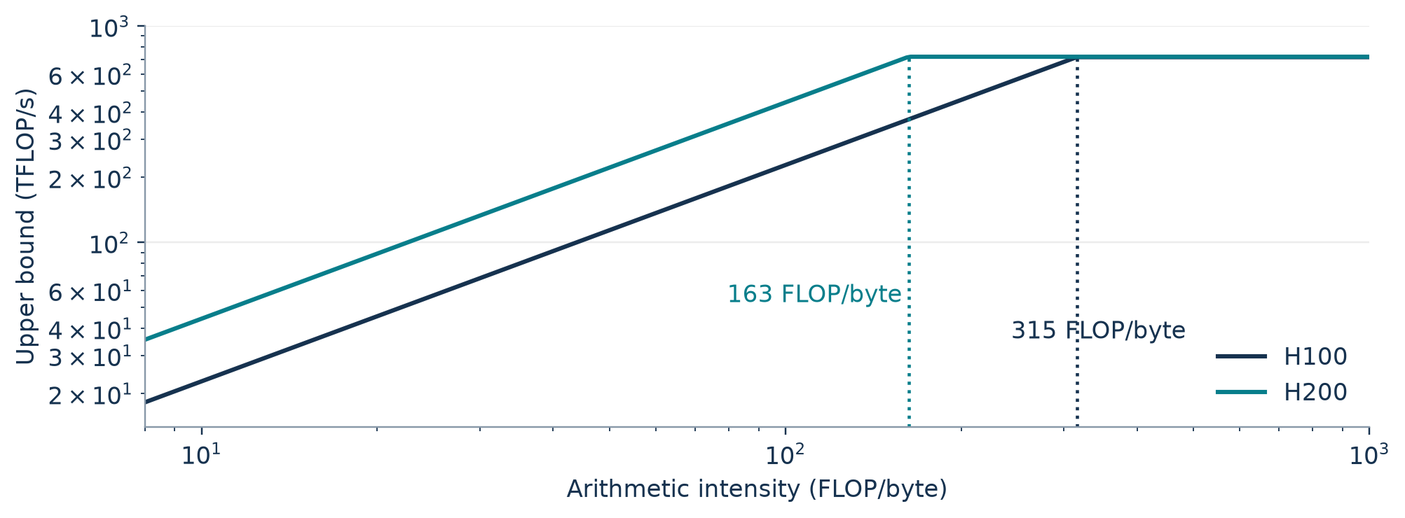
Figure 4. Original roofline using the calibration rates in Section 3. Lines are ideal bounds computed from those rates. They are separate from the paper’s measured step intensities in Figure 6.

A second derivation shows what the simple model would imply for a hypothetical budget. Equate Equation (7) to $I_*$, move the cache term to the left and solve for a batch threshold.

$$\begin{aligned} B(c v-I_*K(L)) &= I_* W,\\ B_* &= \frac{I_* W}{cv-I_*K(L)} \quad\text{when }cv>I_*K(L). \end{aligned} \tag{9}$$

If the denominator is zero or negative, the simplified workload never passes the ridge at a finite batch. A serving trace can still run far below either ceiling because kernel occupancy, launch cost or communication intervenes. Section 9 names attention kernels that stay below the memory roof even at single stream. A roofline locates a resource boundary. To predict joules, Equation (4) still needs round energy and useful output. Energy includes static power, HBM activity, tensor cores, and the fact that the ordinary baseline may improve differently when the GPU changes.

What the counter campaign found

For Qwen3-4B at about 260 tokens of context, the authors report DFlash-16 reaching the H100 balance point at $B=32$ and the H200 point at $B=16$. Its measured energy saving vanishes between 16 and 32 on H100 and at 16 on H200. DSpark-7 remains below the H100 ridge through 64 and saves energy there. On H200 it passes the ridge from 32 and costs energy at 64. The nonspeculative baseline stays below both balance points throughout. An n-gram setting with verified width 16 also crosses H200’s point at 16. At width four it stays below through 64. That comparison helps isolate the shape of the target pass from the identity of the neural drafter.

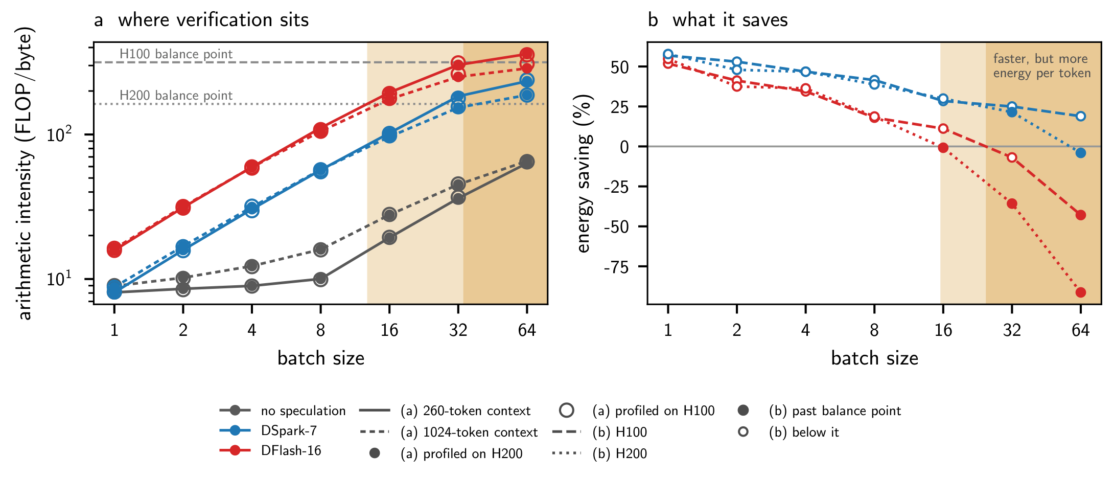
Figure 5. Crop from paper Fig. 6. Qwen3-4B only. Left, arithmetic intensity measured without graph capture at two context lengths. Right, energy savings in the captured serving runs. Follow DFlash-16 across GPU and batch before comparing it with DSpark-7.

The counter profile samples early decode steps after prompts chosen to represent about 260 and 1024 tokens. The shorter prompt approximates the mean context length during the 512-token code generation, but an early-window profile is a local sample at a chosen context. The energy difference integrates a generation. The two measurements need not align exactly even if the hypothesis is right. At 1024 tokens, the additional context reads reduce measured intensity. For substantially longer requests, KV traffic can stay dominant at higher batch. Speculative verification might then share some cache traffic across positions, or it might add substantial memory reads. The short-context crossover cannot settle the direction. MagicDec reports a long-context regime in which speculation improves throughput with little latency sacrifice, a useful comparison for this boundary. MagicDec

A narrower draft can win on memory as well as energy

For a simplified recurrent cache with one snapshot per draft, let $S$ be the sum of the snapshot bytes per request over recurrent layers. If each proposal checkpoint is materialized, the extra snapshot memory is approximately

$$M_{\mathrm{rollback}}\approx B k S . \tag{10}$$

The original boundary state and bookkeeping may consume additional space. A compact representation, partial retention or recomputation would change this expression. The data illustrate the difference between an energy crossover and a feasibility limit. DFlash-16 on Qwen3.6-27B fails to start at batch 16 on H100 even though the ordinary configuration fits. The paper estimates that its rollback buffer alone there is about ten times the drafter weights. On H200 the shorter co-trained head can serve Qwen3.6-35B-A3B at batch 64. A policy should reject configurations that do not fit at actual concurrency before ranking energy.

For MoE the weight traffic also depends on token identities. As an illustrative occupancy model, consider $n=Bv$ routed positions, each independently choosing one of $m$ equiprobable experts. The chance that expert $j$ receives no position is $(1-1/m)^n$. Sum the indicator that it receives at least one.

$$\mathbb E[N_{\mathrm{experts}}] =m\left(1-(1-1/m)^n\right). \tag{11}$$

With eight experts and independent top-one choices, the expected number touched is about 3.31 at four positions and 7.06 at sixteen. Shared routing, top-$r$ assignment, persistent weights and cache locality would all change this toy count. Its purpose is to show why adding positions from one request can still add distinct expert bytes. A dense-layer weight-sharing assumption is a poor proxy in that regime.

Reading the serving experiments

Pairing, metering and the capture counterfactual

A run is a synchronized batch of requests, each producing 512 tokens with no new arrivals. Prompt pools contain 96 distinct prompts per task. Code supplies the full batch sweep and the paper examines conversation, long documents and news in English and Romansh. Weights and KV are BF16, decoding is greedy, and a setting uses at least three seeds. Most runs use one H100 SXM5 with a 700 W power limit. Three batch sweeps use H200 because the weights or large-batch configurations need the additional capacity. Section 9 adds a paired GPU campaign for Qwen3-4B. GPU assignment therefore has to travel with every recorded row. Tables 2 and 3 come from distinct campaigns, and their Qwen3.6 values must stay with their respective GPUs.

The energy counter is sampled at 10 Hz and the difference over a complete generation is used. This cadence can estimate totals over a suitable window. Individual draft and verification phases run too quickly to assign energy to them directly from those samples. The meter covers the GPU board. In particular, CPU work for host n-gram matching is outside the result. If the host adds 0.1 J for each round of a four-request batch committing an average of two tokens per request, the omitted energy is 0.0125 J/output token. That is an illustrative meter-boundary calculation. Whether it changes a ranking depends on the measured board margin and host behavior.

Graph capture is an unusually important control. An ordinary MoE step issues many small operations, so capture reduces baseline launch overhead substantially. The speculative step has already amortized launch overhead over more work. In Table 3 at $B=1$, Qwen3-Coder-30B-A3B-Instruct moves from 71% reported saving with capture off to 32% with capture on. From the rounded table entries, the captured baseline uses 1.60 J/token and the captured speculative run 1.12 J/token, giving 30% from these rounded aggregate values. The paper reports 32% as the median of per-seed paired savings. A ratio formed from rounded aggregate entries is a different estimator. At batch 64 the same row reports 43% and 46% for the off/on settings. Both the scale and the direction of the difference depend on the operating point.

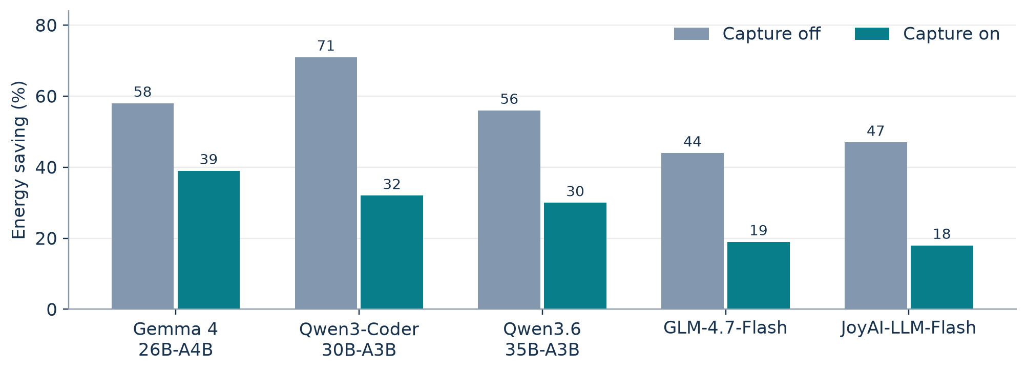
Figure 6. Original redraw of the five MoE rows at batch one in paper Table 3, using reported median paired savings. The gap reaches 39 percentage points on Qwen3-Coder. The JoyAI comparison is on H200.

A useful decomposition of the capture effect is to write $r_0=e_{0,\mathrm{on}}/e_{0,\mathrm{off}}$ and $r_s=e_{s,\mathrm{on}}/e_{s,\mathrm{off}}$ for matched runs. Then

$$\frac{e_{s,\mathrm{on}}}{e_{0,\mathrm{on}}} =\frac{r_s}{r_0}\frac{e_{s,\mathrm{off}}}{e_{0,\mathrm{off}}}. \tag{12}$$

The apparent speculative benefit shrinks when capture reduces the ordinary baseline proportionally more, because $r_s/r_0>1$. This also explains why removing launch overhead from a benchmark can change a scheme ranking. There is no universal adjustment that can be applied to numbers collected in eager mode.

Which drafter wins and why

Table 2 illustrates why one should retain the scheme behind each entry. For Gemma 4 12B, the best reported saving falls from 75% with DFlash at batch one to 25% with the assistant at batch 64. The DFlash drafter verifies 16 positions and the assistant verifies six. On the code pool, longer drafts buy enough output at low batch to offset their extra work. By batch 32, the shorter head leads. On conversation the two schemes advance by roughly the same reported accepted length, and the assistant leads at all measured batches. The longer width still incurs its verifier cost. In the separate fixed-block comparisons on Qwen3-4B and Qwen3-8B, DFlash-7 uses less energy than DFlash-16 throughout the measured sweep. The paper trains neither width variant in a controlled shared recipe, so the result establishes a deployment choice for the tested artifacts.

Qwen3-Coder on code shows an opposite trend to several dense models. Its best reported saving rises from 32% to 51% between batches one and 64. In conversation, the authors report approximately 2.0–3.0 tokens of acceptance versus 5.9 on code, and the same DFlash drafter incurs an energy penalty at batch 64. MoE routing, launch capture and domain all matter. Averaging these settings into one energy curve would remove precisely the interaction the paper exposes.

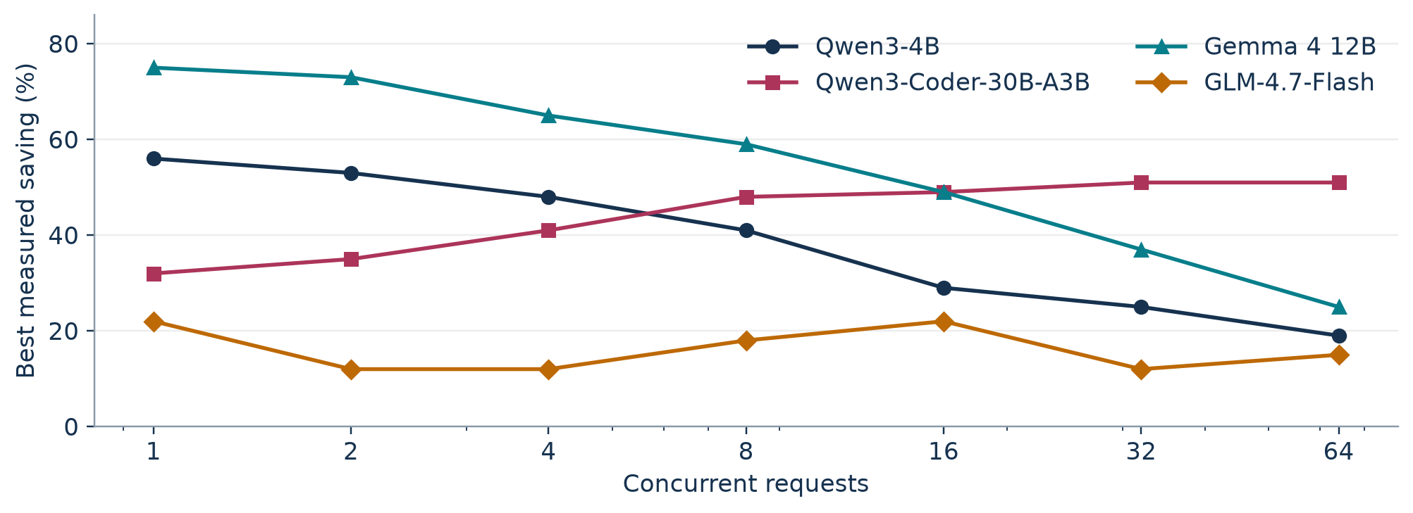
Figure 7. Original redraw of four rows from paper Table 2. Each point selects that batch’s best measured drafter. The curves show the reachable envelope in this sweep and can switch schemes.

In Section 7, a higher accepted length coincides with lower energy in 287 of 332 within-model, within-batch pairs. That is 86.4% by direct division. Of the 45 exceptions, 44 use a higher verified width on the scheme with greater acceptance. The remaining reported pair involves a sequential EAGLE3 draft on Qwen3-8B at batch one. The pairs share baselines and checkpoints. Treating 332 as an independent sample size would understate uncertainty. Their value is diagnostic. A model of energy needs acceptance plus cost and has to recognize the number of sequential draft passes.

What a width sweep can isolate

Section 6.1 sweeps n-gram proposal lengths from 1 to 32 on three targets at four batch sizes. On dense Gemma 4 31B, longer proposals help at single stream. At batch four the best measured length in that sweep is four proposed tokens. At serving batch all swept lengths cost energy, and the longest is the most expensive on that dense target. The two MoE targets have an energy penalty at all swept lengths at single stream. At batch 64 the least costly setting in the sweep is four on all three models. These are the proposed-length labels of that sweep, separate from the verified-width labels in Table 1. A sweep with a host lookup drafter removes neural drafter compute from the GPU comparison, although verification still sees different token content and the CPU meter is still missing.

Observation	Comparator in the paper	What it identifies
Sign change after raising batch	Same target and scheme at paired ordinary baselines	Whether added verification can still pay for its committed output
Different crossing on H100 and H200	Qwen3-4B on two GPUs at matched widths	A change in the resource boundary, alongside GPU-specific baseline energy
Throughput improves but energy rises	Captured energy and separate timing for the same setting	The joint effect of power and committed output rate
Requested batch fails to run	Actual held concurrency and memory capacity	A feasibility limit, with no energy estimate at the requested point

Separating draft energy from verify energy

Section 8 repeats the speculative run while skipping draft passes after the first step, reuses the original proposal shape and fixes acceptance so the two runs have comparable context progression. Let $J_{\mathrm{full}}$ and $J_{\mathrm{skip}}$ be the total energies over those matched windows. Its marginal estimate is

$$\widehat{J}_{\mathrm{draft}} =J_{\mathrm{full}}-J_{\mathrm{skip}} . \tag{13}$$

Interpreting the difference as draft energy assumes the intervention preserves the energy cost of verification. The dense substitution test on Qwen3-8B changes verify energy by under 3% when proposals are replaced by random or repeated tokens. On GLM-4.7-Flash the corresponding change can reach 52%. Different tokens select different experts. The paper consequently reports the split only for dense targets. Even there, the estimate includes interactions such as residency and clocks that change when the draft is removed. It is a useful counterfactual and does not assign a joule to each individual kernel.

The largest measured draft share on dense targets is 45%, and the largest block-draft share is 23%. If the verifier and the number of outputs stayed fixed, halving a 23% component would reduce total energy by 11.5%. The share generally stays similar or falls with batch. A lower-power draft can matter greatly when it improves acceptance or permits a different verification width. Its direct isolated saving alone is bounded by its share.

Language, domain and a selection effect

The matched English and Romansh news test restricts the reported results to outputs that remain in Romansh, determined with function words. On GLM-4.7-Flash and Qwen3.6-35B-A3B the co-trained heads retain 81–84% of their English accepted lengths. The paired post-hoc drafters retain about 70%. GLM’s two compared heads verify four positions each, which removes one width difference. On Gemma 4 12B the vendor assistant and third-party DFlash retain 66–69%. The assistant’s training timing is a better description of this comparison than its vendor origin. The paper reports only 7–11 qualifying outputs per model and drafter at batch one. Qwen3-14B also drifts into Italian in 23–27% of responses. The language-conditioned result is informative about kept responses and cannot estimate the frequency or energy of drift in a live population without restoring the excluded cases.

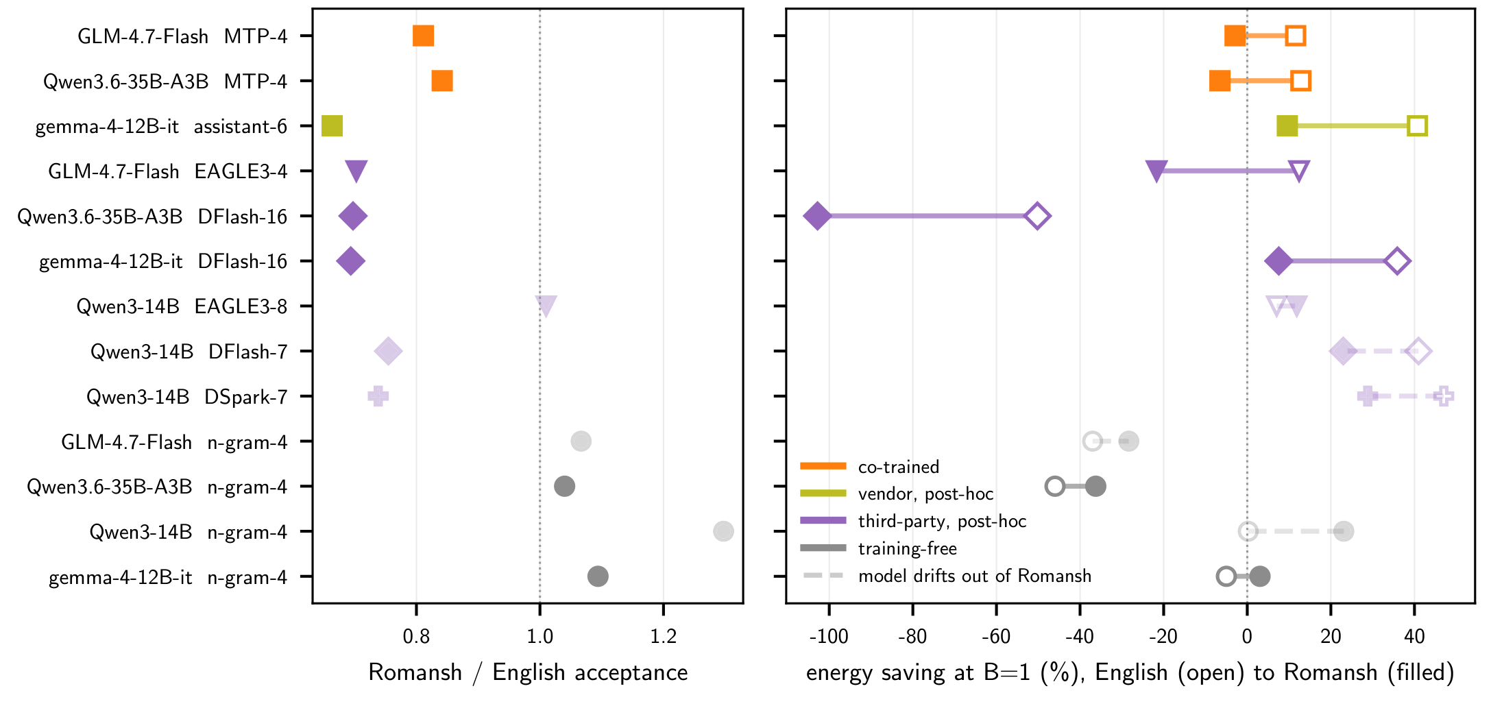
Figure 8. Crop from paper Fig. 3. Follow each row from English to Romansh on the right. The left panel normalizes accepted length to English. Pale rows indicate a target that did not consistently stay in Romansh.

Serving under a latency constraint

For a fixed batch, let $Q$ be aggregate output throughput, $q$ mean throughput per request and $\ell$ mean time between output tokens. In a synchronized run with roughly equal request lengths and matching timing scope, $Q\approx Bq$, $\ell\approx 1/q$ and $e_{\mathrm{out}}=\bar P/Q$. Raising $B$ often reduces the last ratio while raising the mean interval. This relationship also explains why single-user latency and aggregate throughput can both be reasonable optimization targets for different services. They imply different constraints.

A paper Table 4 example is Gemma 4 31B. The ordinary mean intervals at $B=1,32,64$ are 33.2, 38.3 and 56.6 ms. The fastest measured speculative intervals are 7.8 ms with DFlash at one, 19.0 ms with the assistant at 32, and 28.9 ms with the assistant at 64. Among those rows, speculation makes a 25 ms target feasible while batch 64 remains outside it. Across the full sweep, the paper reports energy savings of 18–69% under a 25 ms mean objective for ten models with a feasible ordinary baseline. Gemma 4 31B had no feasible ordinary point. A fastest scheme in Table 4 and an energy-minimizing scheme in Table 2 are different selectors. One should form a feasible set from paired time and energy measurements per scheme, instead of joining their minima by batch.

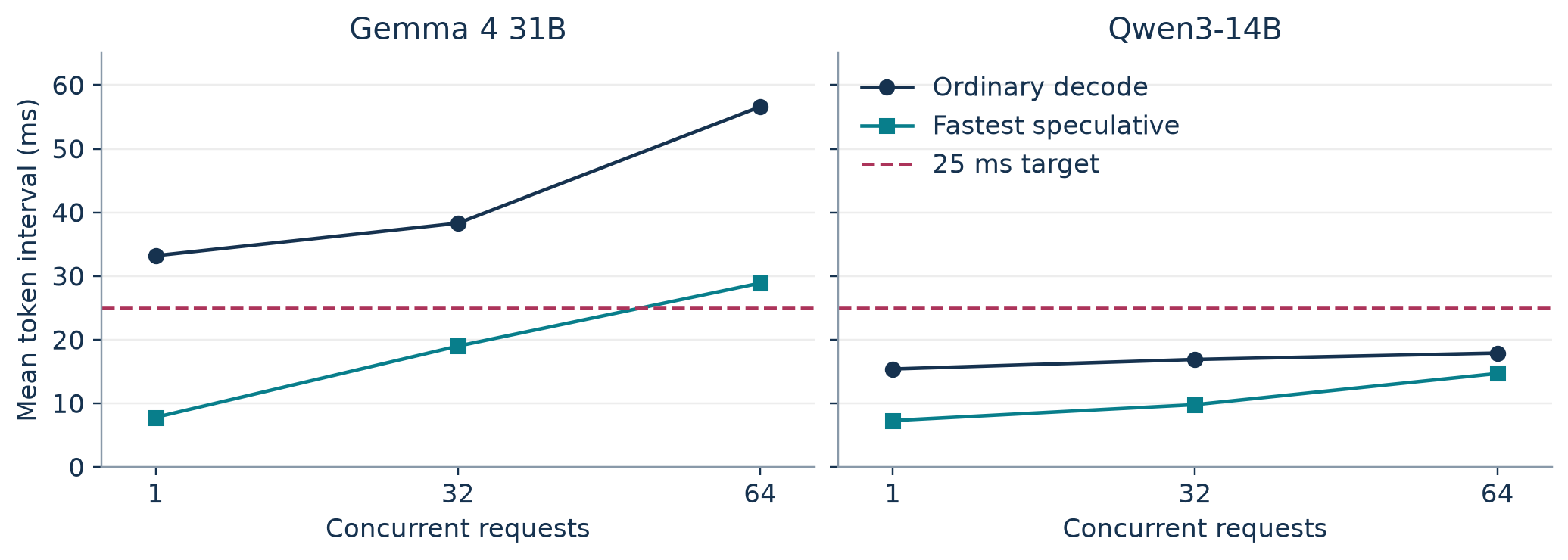
Figure 9. Original redraw from Table 4 for Gemma 4 31B and Qwen3-14B. The speculative markers show the fastest scheme. The dashed line is the 25 ms mean time-between-token target used in Section 5.

The paper reports that single-stream speculation matches the energy of ordinary batching at 2–8 requests, depending on the model. For speculation at batch 32, the ordinary batch required is at least 64, and the baseline at 64 still uses more energy on five of eleven models. These are comparisons on the measured grid. They do not identify a continuous optimum or a threshold at batch 48. At a lightly loaded service, the larger batch also requires arrivals. Waiting to create that batch may consume the latency headroom, and its idle time affects fleet energy. Lower SM clocks are a third lever. On Qwen3-8B on H200, a 1500 MHz lock saves 4–11% on the ordinary baseline at a throughput cost of 3–7%. At batch 16 and above with DSpark-7 or DFlash-16 it offers no additional energy savings in that setting. The 1200 MHz lock lowers both energy per token and throughput. An operator would evaluate the clock together with draft width and actual latency feasibility.

Algorithm 2. Select an energy-efficient feasible serving point

1. Partition observations by target, GPU, context band and traffic class.
2. Define latency and output-quality constraints and the meter boundary.
3. Measure actual batch, mean and tail latency, output count and energy.
4. Pair each draft configuration with the ordinary decode at equal load.
5. Exclude configurations with a mismatch, OOM or failed latency objective.
6. Compare total energy per output token across the feasible batch grid.
7. Retain a baseline fallback and validate the choice on held-out arrivals.
8. Retune when the context, workload or captured shape mix changes.

This is a deployment analysis procedure derived from the paper’s comparisons. The paper itself measures mean intervals. Step 3 asks for additional measurements before transferring the procedure to a tail-latency SLO. An online controller would also need hysteresis. A setting should persist long enough to amortize switching costs, and the controller needs separate responses to a true load change and to noise in estimated acceptance.

Limitations of the measurements

The reported steady batch has no arrival process. It largely isolates the decode mechanism and omits a scheduler’s response to changing prompt lengths, early endings, speculative failure bursts and concurrent prefills. The 512-token cap makes denominators comparable. It can change what is being generated if it extends past an answer’s natural end. The authors check the code pool, where the median uncapped answer length exceeds 700 tokens across models. A median cannot rule out a shorter-answer tail. Long document inputs and realistic output-length distributions also need their own analysis.

The study uses one GPU per run and usually short contexts. Tensor and expert parallelism add collective or routing communication, potentially making verification wait at a different point. The roofline evidence covers one target. H100 and H200 can also differ in board power behavior and baseline speed. A balance point is a plausible explanation of the observed transition within these settings, and there is no estimate here of its predictive error on new models or GPU generations.

The reported half-ranges in Table 2 summarize observed seed variability. They are neither confidence intervals nor a sampling model for new traffic. The paired comparisons control many run-level differences. Selecting the smallest measured energy per batch from a collection of schemes can still favor a noisy minimum. With three or a few seeds, a one-point advantage is weak evidence of a stable serving choice.

Critical analysis

The missing tail is part of the mechanism

A multi-token verification cycle emits in bursts. An average can divide a long silence by many nearly simultaneous tokens. Two streams with the same mean may consequently feel different to the user. Consider an idealized cycle that emits four tokens every 40 ms in one burst. Treat all intra-burst intervals as zero. The mean interval is 10 ms over repeated cycles, while a quarter of intervals are 40 ms. A service that emits one token every 10 ms has the same average and different tail. The paper’s means cannot distinguish these streams. Network buffering and detokenization may change the distribution again. A practical replay would record both individual chunk arrival timestamps and token counts per chunk, and report mean, P95 and the largest or P99 inter-chunk gap, with TTFT recorded separately.

Mean latency can also hide which requests incur the tail. Suppose difficult requests have lower $G$ and thus need more verification rounds before their output completes. Under a continuous scheduler, those requests may be overrepresented in late batches even when initial arrivals are evenly mixed. In a hypothetical single-request model with 200 outputs, average committed advances of four and two translate to approximately 50 and 100 rounds. If the per-round energy is the same, the second class costs about twice the energy per completion. A mixture model for actual observations needs aggregate committed output and time across classes, plus occupancy and fairness constraints. The simple averages in the synchronized sweep cannot supply those quantities.

Use a width experiment that separates proposal quality from the target shape

The strongest causal test would hold target, GPU, graph shape policy and request trace fixed while varying the number of positions the target verifies from the same underlying proposal stream. The paper’s n-gram width sweep tests a useful part of this idea. The fixed block comparisons use different trained drafters. For a sharper counterfactual, I would record a common proposal stream, evaluate early prefixes at multiple widths and measure the whole serving loop separately. Replay can keep each verifier’s prefix and proposal IDs aligned at an evaluation boundary. A live run then shows how changing the emitted advance alters later batching and context. The replay estimate targets the extra verifier cost. The live estimate targets energy per output token after the policy changes the workload it creates.

The serving implementation may require separate captured shapes for different widths. Dynamic confidence thresholds would then incur a dispatch cost and perhaps waste positions when requests are bucketed into compatible shapes. The paper’s DSpark confidence-scheduled test on H100 already shows a failure mode. Its cost table makes an extra position sufficiently cheap that all measured requests are still verified at full width, and the serving-batch saving declines slightly. An adaptive policy needs an energy-aware calibration at actual batch and context, with an objective beyond estimated per-step time.

Account for demand mix and delayed measurements

A service should aggregate energy before taking the ratio. For two workload segments with token counts $N_a,N_b$ and per-token energy $e_a,e_b$, summing joules yields

$$e_{\mathrm{mix}}=\frac{N_a e_a+N_b e_b}{N_a+N_b}. \tag{14}$$

If ordinary decode uses 1 J/token on both segments and a drafter saves 0.4 J/token on code but adds 0.2 J/token on conversation, the energy saving changes sign when the code share of output tokens crosses one third. Those numbers are illustrative. The calculation assumes independent segment energy and fixed segment rates. In shared MoE batches, mixed routing and head-of-line effects can change the component costs themselves. A follow-up should compare mixed replay to the value predicted from homogeneous slices. A gap then identifies workload interaction in the scheduler or expert traffic.

Meter sampling also constrains online control. A slow cumulative meter is useful over a long enough observation window. It gives a delayed response to a policy change. If batch or width changes faster than the window, one reading combines several policies. A controller could use short-timescale signals such as verified width, actual batch and committed advance to predict a setting, with periodic longer-window paired measurement for calibration. It should defer claiming an improvement when the separation between options is below measurement variability.

Strengthen the language and energy attribution experiments

The Romansh comparison would benefit from reporting both the selected and full populations. For the full population, retain energy, accepted length, output language and continuation quality. Stratify by target and compare translations or topics in paired prompt families. Report how many prompts are excluded and why. Language drift can correlate with predictability, so filtering on it can change both the energy distribution and the apparent training-timing effect. Equal-width co-trained and post-hoc heads on several targets would improve separation of training data, tokenizer effects and architecture. The current evidence motivates that experiment and does not identify their independent contributions.

For the attribution experiment, hold actual token IDs and per-expert assignment fixed if possible in a verify-only replay, then compare with the proposal run under identical context and capture conditions. Measuring expert weight bytes and expert occupancy alongside energy would test the explanation for the 52% perturbation on GLM. A dense control with the same procedure would reveal how much of the difference comes from synchronization or power-state changes. The direct consequence for deployment is modest and concrete. A speculative policy must be measured with the serving workload it will produce, including the shapes that were captured and the experts that were exercised.

Reproduction notes and numerical checks

I recomputed the two calibration ridges from the reported rates, the paired-comparison proportion, the Table 3 rounded-aggregate example, and the survival and energy examples. These are arithmetic checks. No GPU generation, energy measurement or model training was run for this review.

A comparable measurement campaign would record prompt and output lengths, the actual running concurrency distribution, scheme and verified width, output counts, GPU model and power cap, precision, decoding settings, graph mode, and the meter and latency windows. Separate prefill from decode where possible. Keep paired per-seed totals and their capture settings. To estimate tail latency, retain per-response timestamps. Check generated output for early EOS, repeated turns and unexpected language drift. Detect duplicate prompts before measurement and record whether cache reuse is part of the intended traffic. A row that requested 16 but ran at 12 belongs to a different concurrency point. Save the individual pairs before computing ratios.

The study’s measurement discussion describes a case in which omitting the chat template raised apparent n-gram saving on Gemma by up to 117 percentage points. An omitted template changes output and acceptance, so the baseline pairing cannot repair it. It also describes an engine resolving concurrency independently for ordinary and speculative runs, and warns about admitting requests inside the measurement window. These are workload changes with plausible numbers. Meter scope and actual run conditions belong in the experimental result.

Conclusion

The paper makes a useful distinction between verification width and committed advance. A speculative round recovers energy when it buys enough committed outputs for its board cost. The dense results show that verify energy dominates the measured draft component and that wide verification can spend the weight-reuse dividend at large batch. The MoE and language results show why the cost and advance both depend on traffic. A decision about which drafter to use therefore needs actual batch, GPU, context and output domain. Under a mean latency objective, select among configurations measured feasible at that objective. A service with a tail SLO needs burst-aware timing before using the same decision.

References

• Bole Ma, Ayesha Afzal, Jan Eitzinger, Harald Koestler and Gerhard Wellein. The paper reviewed. Figures 3 and 6 are reproduced as attributed crops. Tables 2–4 and Sections 2–10 supply the measured values discussed above. arXiv v1
• Yaniv Leviathan, Matan Kalman and Yossi Matias. Fast Inference from Transformers via Speculative Decoding. The original probabilistic construction. Paper
• Samuel Williams, Andrew Waterman and David Patterson. Roofline. The throughput model behind the balance point. Paper
• Jian Chen, Yesheng Liang and Zhijian Liu. DFlash. Block diffusion drafting. Paper
• Xin Cheng and colleagues. DSpark. Semi-autoregressive block generation and confidence scheduling. Paper