Training–Inference Mismatch in LLM RL: What DLC Corrects

Review date: 2026-11-10 (UTC)
Review author: Zhongzhu Zhou
Paper reviewed: On the Origin and Evolution of Training-Inference Mismatch in LLM Reinforcement Learning
Paper authors: Yu Li, Yufa Zhou, Tian Lan
arXiv: 2610.40945v1
Paper version: v1, 29 October 2026

1. What this paper contributes

A rollout worker can produce data that is off-policy for two quite different reasons. It can compute a different next-token distribution from the trainer even when both start from the same parameters. Or it can still be running yesterday’s policy in the much shorter sense of several optimizer steps ago. Both appear in the same logged ratio. They call for different repairs because only the second is directly amplified by the trainer’s own movement within a synchronization interval.

The paper places a third distribution between the rollout and training distributions: run the trainer with the sampler’s weights. The three log-probabilities form an exact decomposition at a common prefix. The measurements then ask what happens after subtracting the off-policy mean score. Under the controlled numerical mismatch, the residual appears small compared with gradient noise. Under a frozen sampler, a residual that grows with the policy displacement feeds into the next update. The proposed discrepancy-lag correction (DLC) reweights and clips the version-dependent factor, subtracts the mean of that clipped score, and refreshes the sampler when a ratio moment signals loss of overlap.

I find the diagnostic separation more broadly useful than the suggested threshold. The algebra does not depend on model size, but the reported one-half crossing is evidence from a particular training regime. In the main experiments DLC mostly buys fidelity to an on-policy run; in the paper’s timing table it pays for that fidelity with an extra forward and more expensive rollout logging. These are separate outcomes.

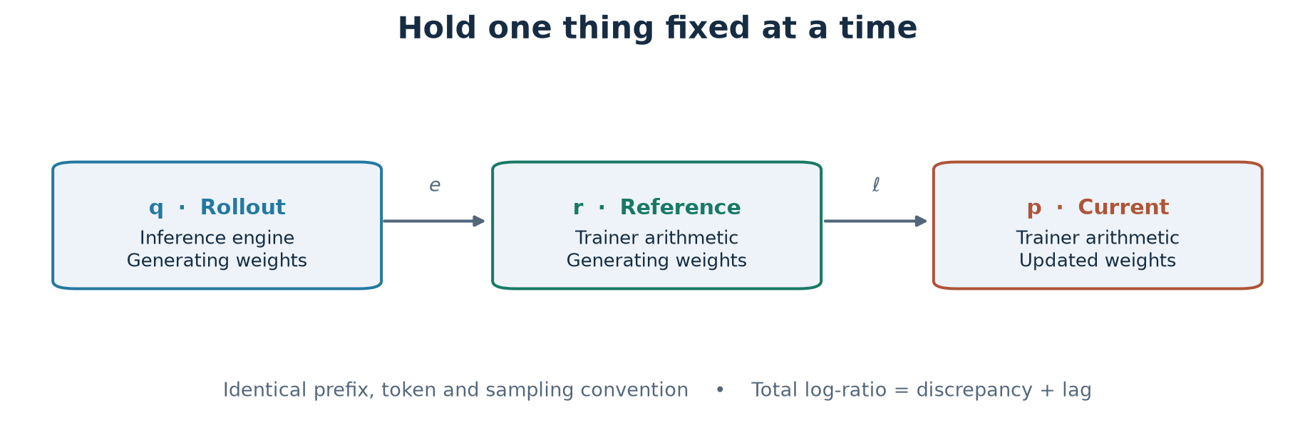
Figure 1. Original diagram of paper Eq. (2). The middle distribution holds weight version fixed against the sampler and engine fixed against the trainer. The tokens and their histories must match in both comparisons.

2. Prerequisites: the data, the score, and the denominator

2.1 Autoregressive actions and group rewards

Given a prompt $x$, write $h_t=(x,y_{<t})$. Each generated token is an action, with EOS or a length cap terminating the trajectory. A policy assigns the response a probability by multiplying its conditional probabilities. Taking logs turns products into sums, which makes per-token evidence easy to collect but does not make the sampled prefixes independent. Early actions determine which later states exist at all. A fix to the distribution of the current token cannot retroactively cause the sampler to visit a different prefix.

In the main setup, eight completions of a prompt receive Countdown rewards of $+1$ or $-1$. The advantage of a completion is its reward minus the group mean, shared across tokens, without standard-deviation normalization. For example, three correct and five incorrect responses give a group mean of $-0.25$ and advantages $+1.25$ and $-0.75$. They sum to zero across responses. Once we condition on a prefix that occurs disproportionately in the correct completions, the mean need not be zero. In addition, token averaging weights long and short responses differently from response averaging. It matters which averaging operation a claim about zero mean refers to.

2.2 Why the expected score is zero

Write $p=p_\theta$ for the training policy and $s_v=\nabla_\theta\log p(v\mid h)$ for the score of token $v$ at a fixed prefix. Here “score” means a vector of parameter derivatives, independent of the reward. For a normalized differentiable distribution on a fixed vocabulary,

$$\mathbb E_p[s]=\sum_v p_v\,\nabla_\theta\log p_v =\sum_v \nabla_\theta p_v =\nabla_\theta 1=0.$$

Let $a_v$ be the expected advantage after choosing $v$ with a specified continuation rule. Adding a constant $d$ to every $a_v$ adds $d\mathbb E_p[s]=0$ on policy. In an off-policy estimate that averages the same score under the sampler $q$, the expectation generally changes. To see the direction of the change, hold $q$ fixed while differentiating:

$$\nabla_\theta D_{\mathrm{KL}}(q\Vert p_\theta) =\nabla_\theta\sum_v q_v(\log q_v-\log p_v) =-\mathbb E_q[s].$$

Add and subtract the product of means in the sampled update:

$$\mathbb E_q[a s]=\mathbb E_q[a]\mathbb E_q[s]+\operatorname{Cov}_q(a,s).$$

The first term is the paper’s drift. In gradient ascent, positive mean advantage pulls the current distribution toward the sampler on that prefix, while negative mean advantage pushes it away. It is possible to get both effects within one prompt even when the prompt-level rewards have been centered. The covariance term is what a change in relative advantages can teach the policy about alternative actions. That term still depends on which measure is used.

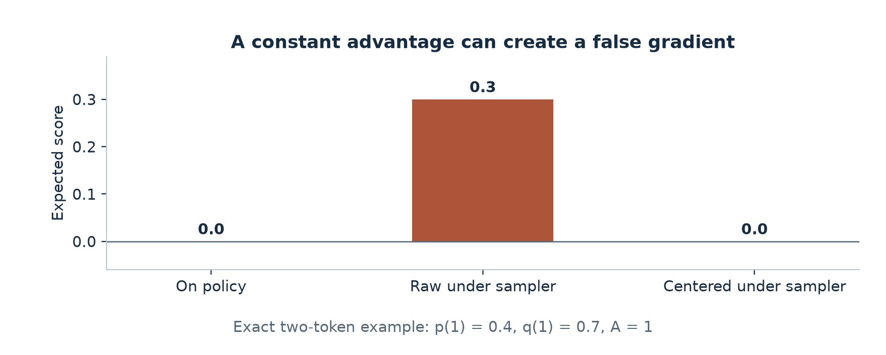
Figure 2. Illustrative exact enumeration. With training probability 0.4 for token one and rollout probability 0.7, the expected scalar score is 0.3 under the sampler. An exact mean subtraction restores zero for a constant advantage; it does not recover the on-policy covariance for a varying advantage.

With the same numbers and $a(1)=1$, $a(0)=-1$, the on-policy gradient for the logit is $2(0.4)(0.6)=0.48$. The exact score-centered update under $q$ is $2(0.7)(0.3)=0.42$. This small example is a useful counterexample to identifying drift removal with unbiasedness. It is also why the paper spends more time on the residual than on proving the mean subtraction identity.

2.3 What importance weighting buys

At a fixed prefix and for a fixed advantage function with $p$ supported by $q$, summing $q_v(p_v/q_v)a_vs_v$ gives the $p$ expectation. With a cap at 2, the difference is explicit:

$$\mathbb E_q[\min(p/q,2)a s]-\mathbb E_p[a s] =-\mathbb E_q[(p/q-2)_+\,a s].$$

The cap trades bias for protection from a small number of very large weights. A token with $q_v=0$ cannot be recovered by changing a weight on observed tokens. A full-response likelihood ratio could in principle also correct where the prefixes and continuations come from, with support and the same definition of the return. The product across a long response can concentrate the weight on a tiny number of trajectories. It can be less usable than a biased local estimator combined with periodically refreshing the data.

2.4 First fix what the probabilities mean

Paper Table 1 is an engineering prerequisite for the analysis. If the sampler reports raw softmax probabilities after drawing from a top-p truncated distribution, the logged denominator is already wrong. If the trainer retokenizes decoded strings, the purported same action and prefix may differ. Reward-conditioned filtering and delayed long responses can change what distribution arrives in the training batch. The experiment uses temperature one, no truncation, shared token IDs and controlled batching. A system with those mismatches still present can compute a numerical difference of logs, but attributing it to precision and version alone would be wrong.

An operator should preserve the actual draw-time version and report the probability of the actual sampling rule. Save positions and completion masks alongside token IDs, and separate the probability of admitting a trajectory from the probability of drawing its tokens. Logging one checkpoint ID per batch is insufficient when a worker can refresh midway through a response. In that case the version belongs to each action, and the prefix is a product under multiple generating policies.

3. Isolating numerical discrepancy and policy lag

Let $r=p_{\theta_{\mathrm{old}}}$ be a forward evaluation using trainer arithmetic at the rollout weights. Define $e$ and $\ell$ at the sampled token, with the same prefix implicit. Adding and subtracting $\log r$ gives

$$\begin{aligned} \delta_t &= \log p_t-\log q_t =(\log r_t-\log q_t)+(\log p_t-\log r_t)\\ &= e_t+\ell_t,\qquad p_t/q_t = \underbrace{r_t/q_t}_{\exp(e_t)}\,\underbrace{p_t/r_t}_{\rho_t=\exp(\ell_t)}. \end{aligned}$$

“Fixed discrepancy” needs a qualifier. For fixed $h_t,y_t,\theta_{\mathrm{old}}$ and engine configuration, changing current trainer parameters cannot change $e_t$. Across prompts, sequence positions, batching, or a refresh of old weights, $e_t$ can change. A stable aggregate around 0.02 nats in the paper’s FP8 condition is an observation about that workload. It is not a theorem that quantization noise is constant or that its alignment with scores stays fixed.

For smooth log probabilities, take $\Delta=\theta-\theta_{\mathrm{old}}$, $s_0=\nabla_\theta\log r$ evaluated at the old weights, and $H_0$ the corresponding Hessian. Taylor expansion gives

$$\ell_v=s_{0,v}^{\top}\Delta+\tfrac12\Delta^\top H_{0,v}\Delta +O(\|\Delta\|^3).$$

If $q=r$, the expectation of the first term vanishes. Differentiating the normalization twice gives $\mathbb E_r[H_0+s_0s_0^\top]=0$. With $F_0=\mathbb E_r[s_0s_0^\top]$, the leading mean and variance follow from the Hessian term and the squared linear term, respectively:

$$\mathbb E_r[\ell]=-D_{\mathrm{KL}}(r\Vert p) =-\tfrac12\Delta^\top F_0\Delta+O(\|\Delta\|^3),\qquad \operatorname{Var}_r(\ell)=\Delta^\top F_0\Delta+O(\|\Delta\|^3).$$

Thus the mean lag can be small even when individual log-ratios have already spread. Summing log-ratios along a response and averaging under $r$ gives the negative sequence KL, by the autoregressive chain rule. This is not the same direction of KL as measuring trained model drift on its own outputs. In the paper’s frozen-sampler runs, the magnitude of the sequence offset grows about 0.7 nats per step, versus a roughly fixed offset in the quantized setting. The two offsets can have similar magnitudes at a particular step but enter the gradients differently.

Algorithm 1. Collect a matched comparison

1. Pin the generating version for each logged rollout token.
2. Save its prefix, token ID, sampled log q and top-H log q.
3. Replay the same token positions in trainer arithmetic at that version.
4. Replay the same positions at current weights; retain their scores.
5. Store e = log r - log q, lag = log p - log r and their sum.
6. Aggregate by version, sequence length and advantage, keeping tails.

Use the sampler’s head $H$ when asking for the reference probabilities; the reference model’s own top tokens can differ. A matched replay on shared checkpoints is stronger evidence for attribution than comparing one trained quantized run to an unrelated trained stale run. It also lets a researcher examine the same token’s ratio before and after a weight refresh, where comparing averages on different prefixes might hide a changing tail.

4. After centering: four residuals and a feedback loop

4.1 Add and subtract one distribution at a time

For plain centering, let $a^\pi$ be the expected advantage when policy $\pi$ generates the rest of the response after the current action. Let $\mu_t^\pi$ denote the prefix law. Write $F(\mu,d,a)=\mathbb E_{h\sim\mu}\operatorname{Cov}_{v\sim d(\cdot\mid h)}(a_v,s_v)$. With exact centering the estimator has expectation $F(\mu^q,q,a^q)$; the on-policy target is $F(\mu^p,p,a^p)$. Insert the two intermediate terms $F(\mu^p,q,a^q)$ and $F(\mu^p,q,a^p)$:

$$\begin{aligned} b_{\rm prefix}&=F(\mu^q,q,a^q)-F(\mu^p,q,a^q),\\ b_{\rm continuation}&=F(\mu^p,q,a^q)-F(\mu^p,q,a^p),\\ b_{\rm token}&=F(\mu^p,q,a^p)-F(\mu^p,p,a^p),\\ b_{\rm tail}&=\mathbb E_{\mu^q}[\mathbb E_q[a^q](\bar s-\hat s)]. \end{aligned}$$

Here the notation suppresses a sum over positions. The last line comes from subtracting a head-based approximation $\hat s$ instead of the exact $\bar s=\mathbb E_q[s]$. For the prefix term, factor the likelihood of each earlier action, so $\mu^p/\mu^q=\exp(S_t)$ with $S_t=\sum_{j<t}\delta_j$. Changing the expectation to $\mu^q$ yields a multiplier $1-\exp(S_t)$. For the continuation term, use the product of ratios over $j>t$ inside the expected return. Those are distinct sources: even when the token being scored has identical probability under both policies, its prior state and downstream consequence can differ.

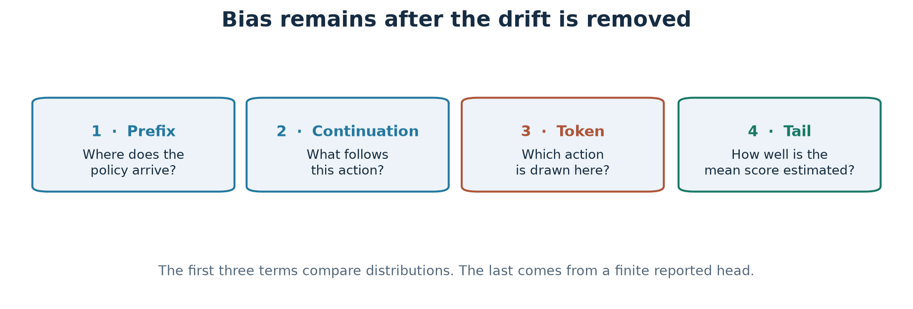
Figure 3. Original schematic of paper Eq. (4). The first three substitutions respectively change where the policy acts, what happens after the action, and which action is selected. The fourth term is an estimation error rather than a change of trajectory law.

For the token term, hold $h$ and $a=a^p$ fixed. The identity $q_v=p_ve^{-\delta_v}$ and the zero $p$ mean of $s$ give

$$\begin{aligned} \operatorname{Cov}_q(a,s)-\operatorname{Cov}_p(a,s) ={}&\mathbb E_p[(e^{-\delta}-1)(a-\mathbb E_p[a])s]\\ &-(\mathbb E_q[a]-\mathbb E_p[a])\,\mathbb E_q[s]. \end{aligned}$$

When the discrepancy is small at that prefix the last product is second order: each of its factors is first order in the change of measure. Expanding the exponential gives $-\mathbb E_p[(a-\mathbb E_p[a])\,\delta s]$. The prefix term expands through $1-e^{S_t}\simeq -S_t$ only when the sum is small. A hundred log differences of size 0.02 with the same sign give $|S_t|=2$, already a poor linearization. The continuation error is also first order in general. The paper’s prediction of the bias keeps the prefix and token terms, and the calculation is therefore a mechanism probe rather than a full approximation with a guaranteed error bound.

4.2 Why lag can amplify itself

Within a frozen interval, for a small displacement $\Delta$ substitute $\ell_t\simeq s_t^\top\Delta$ and $S_t\simeq \sum_{j<t}s_j^\top\Delta$ into the first-order bias. For score centering the resulting operator includes the matrix

$$M_{\rm token} =\sum_t\mathbb E[(A_t-\bar A_t)s_t s_t^\top].$$

The prefix term adds $\sum_t\mathbb E[A_t s_t\sum_{j<t}s_j^\top]$. Untruncated token-level importance weighting removes the token term when there is only staleness, so it keeps the common prefix term in this approximation. For the capped estimator, the omitted token contribution instead contains the factor $(\rho-2)_+ A_t$, as in the exact expression of appendix F. The advantage matters: losing a ratio tail need not bias all gradients in the same direction.

For a projection $u$, the token matrix has quadratic form $\sum_t\mathbb E[(A_t-\bar A_t)(s_t^\top u)^2]$. It can be negative if below-mean advantages dominate along $u$. With $g_k$ the matched on-policy gradient, the update becomes

$$\Delta_{k+1}=\Delta_k+\eta(g_k+b_k) \simeq (I-\eta M)\Delta_k+\eta g_k.$$

A real negative eigenvalue of $M$ yields a factor greater than one in that eigendirection. The prefix matrix need not be symmetric; a negative quadratic form of the token part alone does not prove such an eigenvalue for the whole operator. Finite-horizon amplification can also occur with nonorthogonal modes. I read the sign argument as a concrete mechanism with supporting measurements, not a spectral characterization of the full model.

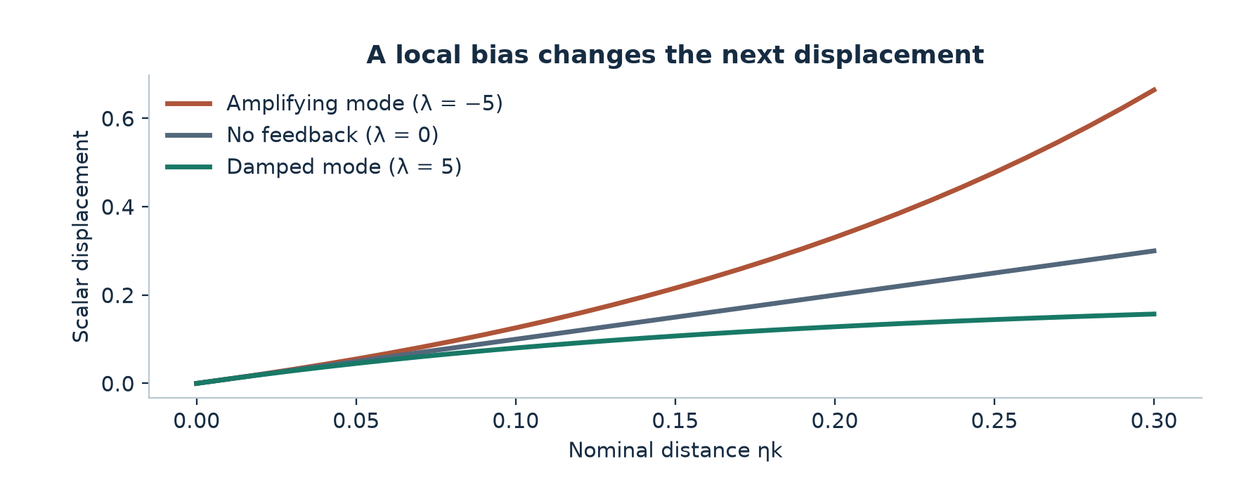
Figure 4. Illustrative scalar recurrence at a fixed gradient, based on paper Eq. (3) and appendix H. The curves are analytic examples, not measured model trajectories.

4.3 Where the quadratic term comes from

Assume $M$ and the mean gradient $\bar g$ are fixed over the interval, with zero displacement after a refresh. Recursing and expanding each factor in the sum yields

$$\begin{aligned} \mathbb E[\Delta_k] &=\eta\sum_{j=0}^{k-1}(I-\eta M)^j\bar g\\ &\simeq \eta k\bar g-\eta^2\tfrac{k(k-1)}{2}M\bar g . \end{aligned}$$

The coefficient counts pairs of steps: a movement created earlier enters the bias of each later step. For small $\eta$ at fixed $\eta k$, it becomes approximately $(\eta k)^2/2$ in magnitude. To compare the norms, linearize $\|x+y\|$ about $x=\eta k\bar g$, so the change is $x^\top y/\|x\|$. Thus the excess norm of the centered estimator over the weighted estimator has leading coefficient $-\bar g^\top M_{\rm token}\bar g/(2\|\bar g\|)$ in the continuous-step approximation. A constant bias would instead add a displacement proportional to $\eta k$. This is a local discriminator; curvature in the on-policy gradient itself, optimizer memory, or changes in the data law also create nonlinear time dependence.

Paper Figure 3 reports a positive quadratic coefficient of 0.52 in a joint fit over two learning rates, with $R^2=0.987$ versus 0.90 for a linear fit. The appendix G norm check is more sobering than the fit: for stale score centering at step 40, the linearized estimate has norm 3399 times the measured bias. Replacing linearized likelihood factors with exact ones reduces this ratio to 6.1, with cosine 0.09 against the paper’s gradient-noise reference of at most 0.07. At step 20 the exact-weight ratio is 4.1 with cosine 0.28. The exact-weight calculation still substitutes sampled $A_t$ for the unknown prefix-centered advantage and omits continuation. A good fit in accumulated norm and a poor fit for individual update magnitudes can coexist.

5. Importance weighting fails at the tail

With a common engine and shared support, $q=r$ and $\mathbb E_r[\rho]=1$. Expanding the square in $\sum_v (p_v-r_v)^2/r_v$ gives $\sum_v p_v^2/r_v-1$ because the cross and constant terms sum to $-2+1$. Thus

$$\mathbb E_r[\rho^2]=1+\chi^2(p\Vert r),\qquad \mathrm{ESS}_{\rm frac}=\frac{(\sum_i\rho_i)^2}{N\sum_i\rho_i^2} \longrightarrow \frac{\mathbb E[\rho]^2}{\mathbb E[\rho^2]}.$$

Here $N$ counts sampled tokens, and the limiting moment statement needs enough representative samples. The name ESS describes concentration of weights, not the number of independent gradient observations when multiple tokens come from the same completion. The paper uses the reciprocal second moment $1/\mathbb E_q[\rho^2]$ as its trigger. With quantization, $q\neq r$, and the lag ratio need not have mean one under $q$. A reciprocal moment and a normalized Kish statistic then answer different questions. For example, if every logged ratio were 1.5, the former would be 0.444 and the latter one. Such a uniform factor cannot hold over a complete common-support $r$ vocabulary, but can describe a sample biased toward one region.

For the Gaussian comparison, assume $\ell$ has mean $\mu$ and variance $\sigma^2$. The identity $\mathbb E[\exp(c\ell)]=\exp(c\mu+c^2\sigma^2/2)$ first gives $0=\mu+\sigma^2/2$ at $c=1$, then $\log\mathbb E[\rho^2]=2\mu+2\sigma^2=-2\mu$ at $c=2$. So the one-half crossing is at $-\log 2/2$, or about $-0.347$ nats. If $K(c)=\log\mathbb E[\exp(c\ell)]$ has a convergent cumulant expansion at both arguments, $K(2)-4K(1)$ cancels the variance term while leaving third and fourth cumulants with coefficients $2/3$ and $1/2$. This shows how the upper ratio tail can reduce ESS even at the same mean log-ratio. Neither a Gaussian fit nor a check of only the low-ratio tail is a substitute for measuring the second moment.

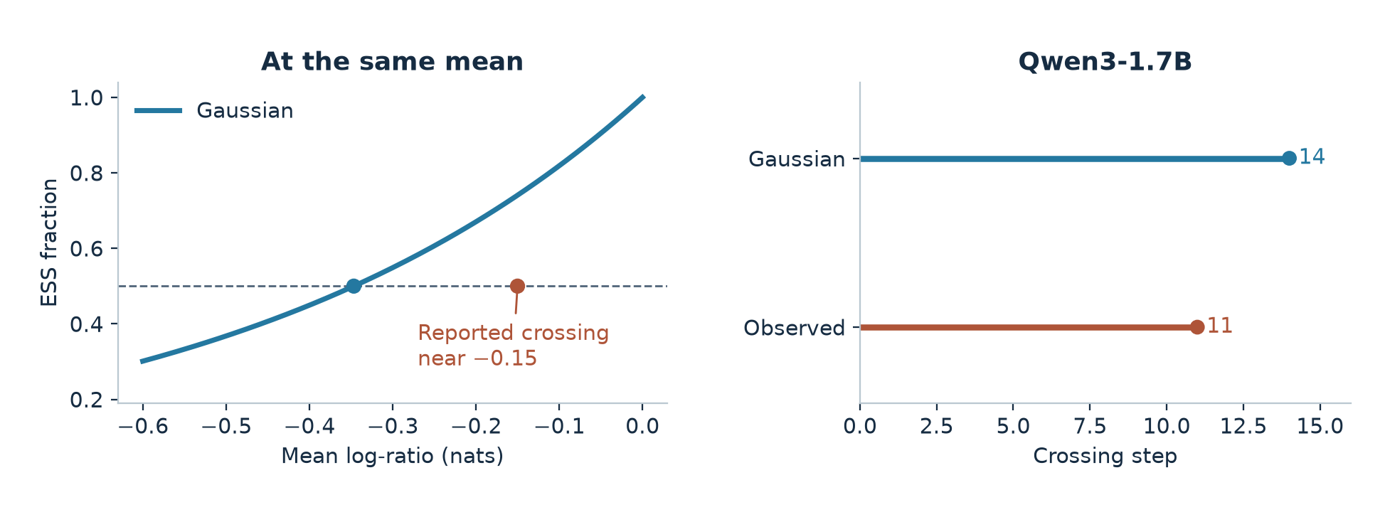
Figure 5. The curve is a Gaussian calculation from paper Eq. (32); the observed marker records the reported crossing near mean lag −0.15 on Qwen3-1.7B. The second panel marks reported steps from paper Fig. 4(b), not a reconstructed time series.

On Qwen3-1.7B, the measured moment passes the threshold at step 11 rather than step 14 predicted by the Gaussian approximation. At $\mu=-0.15$, the Gaussian fraction would still be about 0.741. Using the crossing as approximately one half implies an excess log second moment of $\log 2-0.30\simeq 0.393$. A separate observation for Qwen3-0.6B: at step 40, the observed fraction of ratios below 0.5 is 11% versus 28% under its matched Gaussian. These observations involve different model sizes and different parts of the distribution. The 0.6B tail count does not by itself establish why the larger model crosses early.

6. Building the DLC update

6.1 Clip the lag, not the combined discrepancy

The denominator is the design choice. A weight $p/q$ contains both factors; truncating it can cut a token purely because of numerical error. A PPO ratio with a before-batch reference is exactly one at the first update of a batch even when the data were sampled many versions ago. Subsequent inner updates bound movement relative to the before-batch policy, not relative to the generating version. DLC uses $p/r$ and a sign-dependent PPO gradient mask:

$$m_v= \begin{cases} \mathbf 1\{\rho_v\le 1+\varepsilon\}, & A_t>0,\\ \mathbf 1\{1-\varepsilon\le\rho_v\le c\}, & A_t<0 . \end{cases}$$

For $A_t=0$ the term contributes zero. Paper values are $\varepsilon=0.2$, $c=3$. The mask describes where the gradient of the piecewise clipped surrogate is active, not a replacement of $\rho_v$ by its clipped value in the gradient. For example $\rho_v=1.35$ is dropped when the sampled advantage is positive, yet remains active when it is negative. For a given position, the same sign must determine the mask of each head candidate in the centering term; changing the sign changes which mean is being subtracted.

6.2 Recover a weighted mean from the top of the vocabulary

DLC wants to subtract $C=\sum_v q_vm_v\rho_vs_v$. Only the head probabilities of $q$ are available for the counterfactual actions. Define $\kappa=(1-\sum_{v\in H}q_v)/(1-\sum_{v\in H}r_v)$. Approximate $q_v$ by $\kappa r_v$ in the tail and use an inactive clip in the approximation. Then the estimated tail coefficient is $\kappa r_v(p_v/r_v)=\kappa p_v$. Because the full $p$-weighted score sums to zero, the approximate mean can be computed from the head:

$$\begin{aligned} C &\simeq \sum_{v\in H}q_vm_v\rho_vs_v+\kappa\sum_{v\notin H}p_vs_v\\ &=\sum_{v\in H}(q_vm_v\rho_v-\kappa p_v)s_v,\qquad \hat g_{\rm DLC}=\sum_t A_t(m_t\rho_t s_t-C_t). \end{aligned}$$

Here $C_t$ denotes the head estimate on the right. As in paper Eq. (6), Algorithm 1 and appendix L, the advantage multiplies both terms. This shared factor makes constant-advantage cancellation possible. The approximation avoids reporting a full rollout vocabulary at every token and still uses the actual sampled ratio and mask for the sampled action. If the actual tail is not proportional to the reference or contains strongly clipped ratios, the mean subtraction leaves a residual. An adaptive head that targets retained probability mass can be more informative than a fixed count, at the cost of variable logging and padding overhead. Very small denominators in $\kappa$ also need a numerical policy; matching two nearly zero masses by subtraction can lose precision.

6.3 What cancels, and what stays

Inside the active mask, $q_v\rho_v=p_ve^{-e_v}$. The lag no longer appears explicitly in the action weight. At a fixed prefix, with exact centering and fixed advantage function, compare the $q$ weighted update to the on-policy one by subtracting and adding the on-policy mean advantage:

$$\begin{aligned} b_{\rm tok,DLC} ={}&\mathbb E_p[(e^{-e}-1)(a-\mathbb E_p[a])s]\\ &-(\mathbb E_q[a]-\mathbb E_p[a])\mathbb E_p[e^{-e}s]. \end{aligned}$$

The first term is primarily a numerical residual, of first order in $e$. The second can contain lag through the advantage mean difference, but its score factor is zero at $e=0$ and first order near that limit. This explains the paper’s statement that lag enters that local term through a product with discrepancy. The statement requires an inactive mask and adequate tail information. Clipping gives up part of that cancellation to control outliers. The prefix and continuation distributions still come from the sampler. A refresh cuts their lag component for new samples; it does not fix the engine discrepancy or turn data already generated into fresh samples.

If $\theta=\theta_{\mathrm{old}}$ then $\rho=1$ and the estimator becomes plain score centering with its head approximation. If $q=r$ and the mask is inactive then $\kappa=1$, $C=0$, and the local update is the sampler-reference PPO gradient in its active region. With a nontrivial mask, $C$ can be nonzero even for $q=r$. These limits are useful paper-math checks when implementing a loss from the derivation.

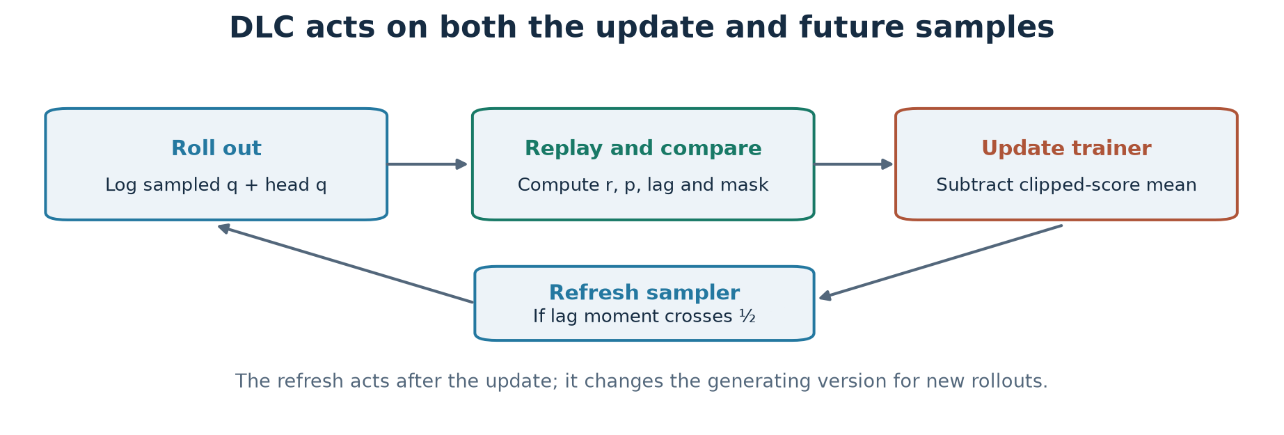
Figure 6. Original diagram of the paper’s Algorithm 1. Reference replay serves the lag ratio and the head estimate. The decision uses the current batch’s unclipped lag ratios and changes future rollouts.

Algorithm 2. One DLC training step

1. Roll out at the recorded sampler version; log sampled and head q.
2. Score the completions and compute each prompt group's advantages.
3. At the logged version, evaluate r on sampled and head token IDs.
4. At current weights, evaluate p; form rho = p/r and the sign mask.
5. Estimate the weighted mean from the head using matched tail mass.
6. Form the stopped-coefficient correction to the PPO loss.
7. Take one SGD step; if reciprocal lag second moment < 0.5, refresh.
8. In a mixed-version stream, keep version per token; separately log
   any response deferral and regeneration under the admission variant.

Appendix L adds $\sum_t A_t\sum_{v\in H}\operatorname{sg}(q_vm_v\rho_v-\kappa p_v)\log p_v$ to the minimizing PPO loss; $\operatorname{sg}$ means stop gradient. Differentiation gives $+\sum_t A_t C_t$; descent therefore subtracts it from the ascent update. Allowing gradients through the coefficients would introduce derivatives of $p$, $\rho$, and the mean estimator that are absent from the intended update. Both loss terms use the same token aggregation. The appendix reports clamping the lag ratio to the range $[e^{-20},e^{20}]$ in the loss. For logging a moment across shards or a long batch, a log-sum-exp reduction and a count of valid tokens avoid overflow; logging pre- and post-clamp statistics would clarify whether extremes or clamping drive a trigger.

7. Experiments: fidelity, reward, and time

7.1 What is controlled

The authors train non-thinking Qwen3-0.6B and 1.7B on Countdown for 40 steps with three runs per main configuration, 64 prompts and eight completions per prompt, 135 prompt and 377 response tokens as the caps. Rewards are binary signed values, with group mean subtraction and token averaging. Trainer compute is BF16 with FP32 master weights and FSDP2; SGD uses learning rate 0.01 without momentum, warmup or weight decay. Selected loop probes use 0.005. The reference uses vLLM BF16 and CUDA graphs. The quantized sampler uses FP8 block weights, dynamic activation quantization and FP8 KV cache; the frozen sampler has a nominal 64-step refresh interval so the unrefreshed 40-step run never gets a scheduled copy.

The authors average full-vocabulary next-token KL from each trained policy to its paired on-policy policy over fixed prefixes generated by the initial checkpoint. The denominator is the mean KL between independently trained on-policy policies. A normalized deviation of one is a calibration point, not a confidence interval, and a value below one does not mean the policies are identical. Accuracy measures the trained model’s own responses on held-out Countdown; the paper evaluates eight responses per prompt on 64 problems. Keep the held-out return, fixed-prefix divergence, and direct runtime cost distinct.

7.2 Quantization and frozen rollout separate the methods

Paper Table 2, Qwen3-0.6B at step 40. Each cell is deviation relative to the on-policy noise floor followed by test accuracy. A dash indicates an unreported configuration.

Method	FP8	Frozen BF16	Frozen FP8
On policy	1.00 / 46.5%	1.00 / 46.5%	1.00 / 46.5%
Plain gradient	12.7 / 26.4%	345 / 0.2%	107 / 0.2%
Truncated IS	0.74 / 43.2%	4.50 / 20.9%	3.91 / 27.1%
Centering	0.80 / 46.5%	31.7 / 12.2%	28.1 / 18.4%
IS + centering	1.11 / 46.0%	2.10 / 32.0%	2.61 / 30.5%
DLC	—	1.93 / 31.7%	2.17 / 30.3%

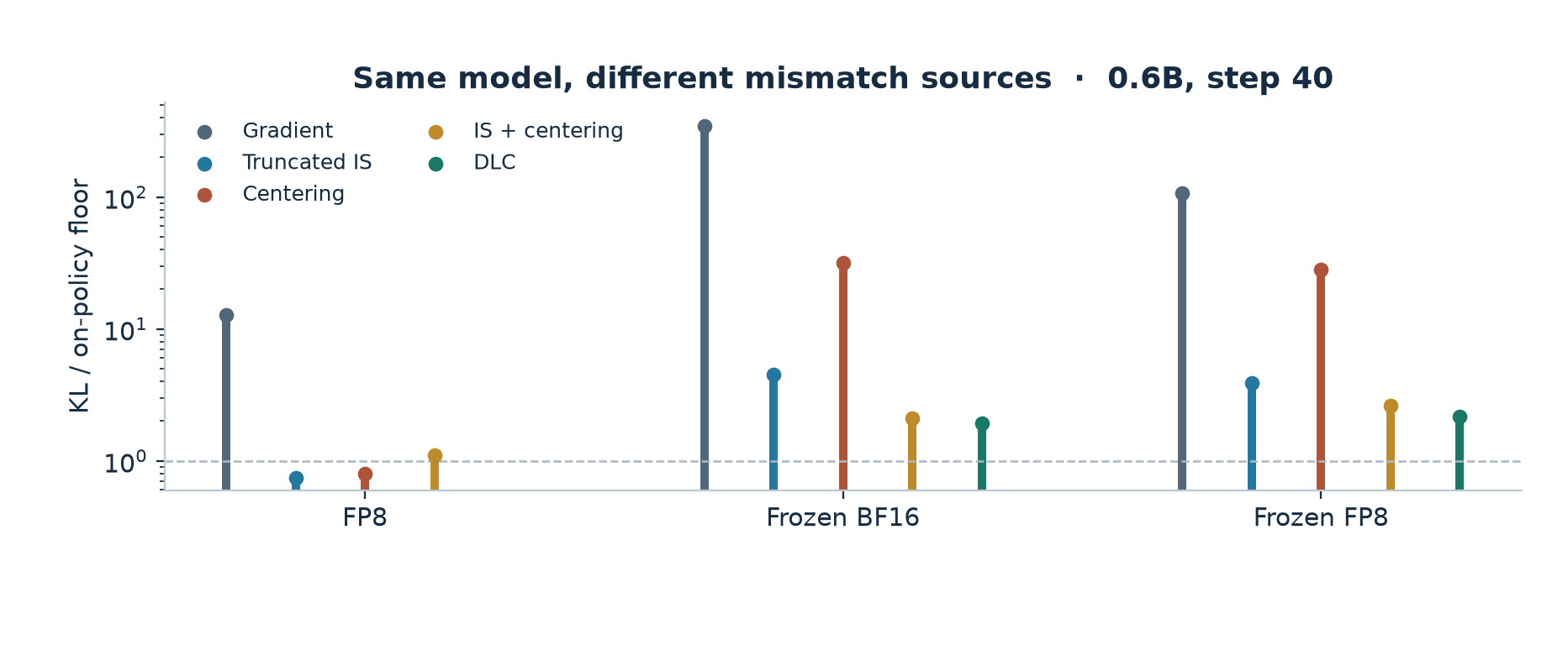
Figure 7. Redrawn from paper Table 2, step 40. The logarithmic vertical scale is normalized KL, and missing configurations have no bar. This is not an accuracy plot.

The ranking reversal for centering versus importance sampling is the main result of this intervention. Centering matches on-policy accuracy for numerical mismatch and finishes 34.3 points below it under staleness. In frozen BF16, DLC improves normalized deviation slightly relative to IS with centering, while accuracy is 0.3 points lower. The aggregation matters: Appendix B’s mean of per-run ratios changes that frozen-sampler comparison from $1.93$ versus $2.10$ to $2.70$ versus $2.51$. I would not use the small difference to decide between the two at this size. The stronger result is that both are much closer to the reference than plain centering in this configuration.

7.3 Refresh ablation, blindness of the fixed probe

For 1.7B with frozen rollout, Table 4 gives DLC 0.6 times the floor and 51.9% at step 40, versus on-policy 57.6%. The three DLC runs refreshed once each (steps 20, 35 and 36). Importance sampling alone reached 115 times the floor and 0.5%; adding the same refresh trigger brought these to 2.6 times and 36.6%, with 2, 4 and 5 copies. The refresh alone therefore accounts for a large part of the recovery. The combination in DLC uses fewer copies in this study and gives better accuracy, but the experiment changes both the estimator and its subsequent refresh schedule.

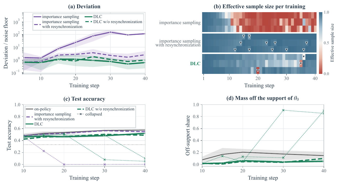
Figure 8. Cropped from paper Fig. 5, p. 14. Compare fixed-prefix deviation in panel (a) with trainer-sampled accuracy and rare-token attribution in panels (c) and (d). Triangles in (b) mark observed refresh events.

Two of three no-refresh DLC runs fall below the initial model’s accuracy. Their fixed-prefix KL stays within the range of learning runs. The authors instead sample from the trainer and decompose its sequence KL to the initial checkpoint by the probability the initial policy gives the chosen token. A chosen token with initial conditional probability below $10^{-3}$ contributes to the numerator of the off-support share. The denominator is the sum of all sampled log-ratio contributions. The collapsed runs reach roughly 90% rare-token attribution, from at most 14% before collapse; full DLC stays at or below 11%. The initial policy can give positive probability to these tokens, so “off-support” is operational shorthand for low probability. Individual log-ratio contributions are signed; the statistic is not the probability of drawing a rare token and can be unstable when total KL is near zero.

7.4 The larger run and the price of the second forward

The 8B frozen test in Appendix C has one run per row. DLC has 3.1 times the floor and 49.6%, while IS with centering has 2.9 and 51.8%; on policy reaches 55.3%. Plain centering has 89.1 times the floor but 51.4% accuracy. That last pair illustrates why a task reward can agree across policies that assign very different probabilities. In continuous asynchrony at 1.7B, the maximum gap is four versions and the token-weighted average is 2.85 versions. One run each yields 1.2 times the floor and 55.9% for DLC, 0.8 and 55.3% for admission DLC, 1.4 and 52.9% for IS, and 56.8% for on policy. Admission deferred 68 responses (reported as 0.3%) over 40 steps and cost 94.2 seconds per step versus 80.1 for DLC and 43.7 for IS. This is promising bounded-asynchrony evidence, with insufficient repetitions for a general throughput or accuracy conclusion.

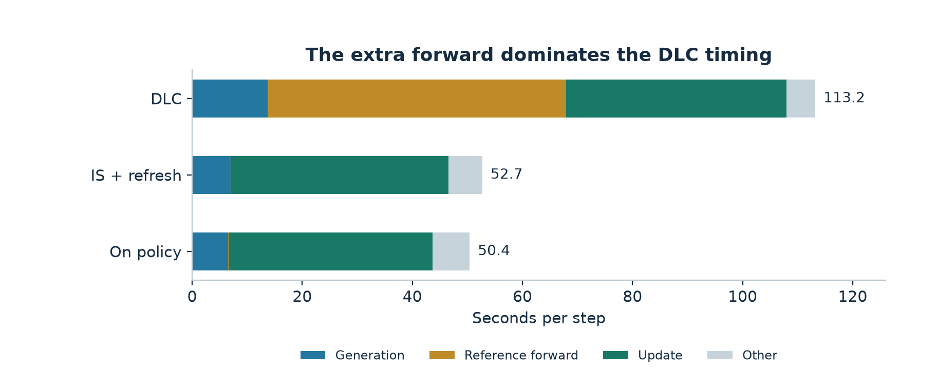
Figure 9. Redrawn from paper Table 7 for frozen 1.7B. The light remainder is reported step time minus the three named components. Synchronization savings do not dominate this setup.

In the stale experiment DLC costs 113.2 seconds per step versus 50.4 on policy and 52.7 for IS with refresh. The reference forward accounts for 54.2 seconds in DLC, and generation 13.7 versus 6.5 seconds on policy. The authors identify about 19 seconds of redundant reference work on an unused KL path. Even subtracting that amount as a rough arithmetic counterfactual, the result is about 94.2 seconds, still 1.87 times the reported on-policy step; this is not a measured optimized runtime. The rare copy is inexpensive on this testbed (at most 1.5 seconds, once per 40 steps for DLC). A distributed system with expensive cross-node weight movement may make a different trade, but the paper does not provide that measurement.

8. Limitations

Coverage. Most evidence comes from one arithmetic task with short capped responses, a narrow family of dense models, a short training horizon and simple SGD. With Adam or Muon, the residual can modify optimizer state and change future steps even after a weight copy. MoE routing changes, stochastic kernels and rapidly drifting precision error can invalidate the empirical stationarity observed for the FP8 configuration. Longer responses increase the opportunity for prefix mismatch and can change which samples dominate token-level summaries.

Precision of the bias diagnosis. The first-order comparison freezes parts of the dynamics and ignores continuation in the predicted bias. Table 10 shows that magnitude prediction remains weak even with exact likelihood terms. Similarly, the Gaussian clipping probabilities in appendix I are marginal ratio probabilities. Turning those into dropped shares by sign requires the sign-conditioned ratio distribution or a suitable independence assumption. Paper Figure 3 itself shows that advantage and lag can be associated. These expressions are useful references for diagnosing tails, not calibrated estimates of how much useful gradient the mask drops.

Reference assumptions. ESS is a marginal overlap statistic, and the paper’s boundary at one half is calibrated on a small set of runs. The approximation for the tail of the clipped mean can fail in low-probability regions. In a mixed-version rollout, normalization for a complete prefix must account for the actual per-token version and preceding actions. Deferring high-lag responses is a data-selection operation: if rejected responses cluster by length, task, or reward, the distribution admitted for training differs from the rollout law.

Evidence about cost and robustness. The large-model and continuously asynchronous rows are exploratory single runs. The paper times steps in its own configuration and does not hold throughput, wall clock, data volume, or quality target fixed across all comparisons. There is no evidence here that one method wins on elapsed time to the same accuracy. The rare-token share was evaluated on a limited number of checkpoints and uses a probability threshold tied to the initial policy. Legitimate exploration can also move into regions that initially had little probability.

9. Critical analysis

9.1 Use a two-view gate with a cost budget

I would treat lag ESS as a warning on the worker’s data, and add a small, independent stream from the current trainer. Estimate the reciprocal moment and Kish fraction on matched tokens, stratified by generating version, response position, prompt class and advantage sign. Bootstrap by response, or by prompt group when using shared group rewards, so a cluster of long completions cannot masquerade as precise evidence. Log the fraction of gradient-bearing tokens dropped by the clip and the sum of their weighted advantages. This makes a case in which ESS is high but the few rare positive trajectories are clipped visible to the operator.

For the second view, periodically sample the trainer on a held-out prompt pool and report task success, length, actual mass at low initial probability, and raw sequence KL before taking a ratio. As an illustration, a prefix that occurs with probability $10^{-5}$ under the old policy and $10^{-2}$ under the current policy would be expected 0.01 versus 10 times in 1000 trajectories. The old probe could miss it while it is routine enough to affect the trainer’s answers. A KL close to the on-policy floor on old prefixes is compatible with this example. Conversely, a rare-token warning without degrading task success could be benign exploration. A two-view gate can refresh or pause data admission when these signals agree and ask for a small fresh probe when they diverge.

9.2 Separate a better estimator from better refresh timing

Use a crossed experiment with the same prompt and seed streams: full DLC, lag weighting without centering, centering without lag weighting, and truncated combined weighting. For each estimator compare frozen, fixed refresh, and adaptive refresh, and add a matched-copy-budget schedule derived on held-out tuning runs. Fixed schedules reveal what the estimator buys for an identical data age cap; matched adaptive schedules reveal how often each estimator has to pay for a new version. Report all seeds, the full cost of reference replays, and paired uncertainty at a fixed compute budget. Continue past the first refresh so the regime includes multiple cycles.

In the mixed-version case, randomize a fraction of borderline admission decisions for measurement, and record which prompts and lengths are deferred. This gives a way to assess selection bias and whether restarts disproportionately lose slow, difficult responses. For training, make the cost function include wasted rollout tokens and the waiting time of admitted samples. A method that improves fixed-prefix KL but slows down every update may still be valuable in a safety-critical experiment; the appropriate comparator depends on the quality requirement and system budget.

9.3 Probe the mechanism before generalizing it

Measure the projected residual along a fixed gradient or a small set of checkpoint directions, with matched prefix samples, before interpreting a quadratic fit as proof of feedback. Use several synchronization intervals and learning rates at the same nominal distance, plus an intervention that resets just the rollout weights. Re-evaluate the discrepancy on the same prefixes after changing reference version; a large jump there would contradict the practical fixed-offset model even though the three-policy factorization still holds. For head-size sensitivity, report the tail mass and occasionally estimate its weighted score on a small diagnostic vocabulary subset. This can reveal whether a lower or higher top-$H$ is justified by actual score error rather than by an arbitrary token count.

One can choose a budget for comparing approaches before tuning: wall time to a held-out score band with an uncertainty target, or model tokens consumed before a fixed-reference deviation threshold. Report both raw KL and its noise-floor ratio. Above all, keep equal-version engine differences visible in the accounting. A zero version gap with probability errors from precision, normalization or batching is a different state from a genuinely on-policy rollout.

10. Reproduction plan and arithmetic checks

The paper’s main result can be tested with a four-cell intervention: aligned, quantized only, stale only, and combined. Specify the sampler and trainer precision, draw and admission rules, exact versions, evaluation prefixes, group baseline and token reduction. Before comparing methods, measure three log-probabilities at common positions and verify that their split closes at numerical tolerance. Report paired on-policy seeds so that “one times the floor” is reproducible. Then compare drift and prefix/continuation residual proxies on matched checkpoints, and use fresh trainer rollouts to measure exploration and collapse. No model training was rerun for this review.

For arithmetic checks, I enumerated the two-token score example, verified the sign and finite-difference limit of the logit gradient, and computed the Gaussian crossing, the estimated tail excess, and table differences. A useful test of the centering loss on a small vocabulary is to replace advantages by a fixed constant and compare the expectation before and after subtraction. A useful test of the resynchronization derivation is to set $p=r$ without setting $q=r$: the lag should vanish, while the numerical discrepancy can remain. These tests check the equations and assumptions in the review; they do not establish the paper’s model-level outcomes.

11. Conclusion

DLC makes a helpful distinction between correcting a statistic of the current batch and changing what will be sampled next. The reference forward identifies a version ratio that can be clipped independently of numerical error; subtracting its weighted mean handles the constant-advantage part of the remaining update; resynchronization changes the future sampling law once overlap degrades. This sequence explains why simple centering works in the paper’s FP8 setting and fails in a frozen rollout, and why a stable fixed-prefix KL is insufficient evidence of a healthy policy. The next question for a larger system is whether this extra reference information and the adaptive refresh pay for themselves at equal time and target quality.

Primary sources: Li, Zhou and Lan, arXiv v1, sections 2–7 and appendices A–L; PPO; DeepSeekMath / GRPO.