FLAMIA | When the quantizer is part of the causal mask

Review date: 2026-11-08
Author: Zhongzhu Zhou
Paper reviewed: FLAMIA: FLAsh MIcroscaling Attention for Fast and Causally Safe Training on Blackwell
Paper authors: Fedor Velikonivtsev, Mikhail Koltakov, Denis Kuznedelev
arXiv: 2611.03344, version v1, 2026-11-02

1. What changes when attention goes low bit

Consider a query at the beginning of a training sequence. Its attention mask prevents it from reading later values. Before the mask acts, a quantizer may nevertheless inspect those later values to decide how to round the earlier ones. This creates a second dependency graph that the standard causal mask does not describe. A model trained in that graph can learn to use information that will be absent in incremental decoding. FLAMIA makes this problem concrete with a suffix perturbation test and an experiment that evaluates the same weights through two attention kernels.

The paper has a parallel systems argument. In training, a single tensor can feed several matrix products whose reductions run along different axes. Scaling a narrow stripe along one axis is a natural fit for hardware microscaling. A transposed contraction may need an entirely new set of codes, which costs memory bandwidth and can leave the extra tensor-core throughput unused. FLAMIA shares an exponent over regions chosen to survive both orientations. It uses a mixed route when FP4 helps score computation and retains wider formats for other products.

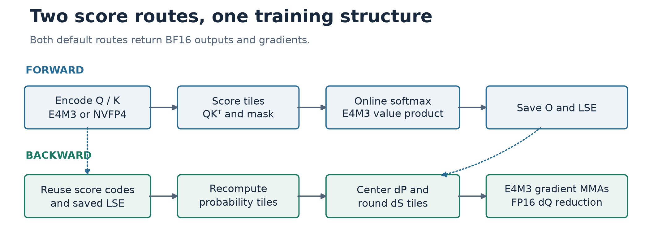
Figure 1. Original schematic based on paper §§3.1–3.5. The upper lane reconstructs scores from the selected Q/K format. The lower lane reuses the same score representation and switches to E4M3 operands for the gradient products.

There are three empirical claims to keep separate. The causal packed training call using default MXFP8 is faster than the fastest evaluated eligible baseline on all nine workloads per GPU. The large training run tests how far loss and downstream accuracy move under that kind of arithmetic. The strict dependency test uses additional options with narrower support than the headline packed benchmark. In particular, the reported exact options currently cover supported batched causal calls. I use “exact” below in the paper’s dependency sense. The arithmetic still uses low precision.

2. Prerequisites

The contraction moves between forward and backward

Let $Q,K,V$ each have $L$ token rows and $d$ feature columns for one head. Let $G$ denote the gradient arriving at the output $O$. Use $\Omega_i$ for the keys visible to query $i$. For ordinary causal self-attention inside one document, those are the keys in that document up through $i$. Define the scaled logits, row probabilities, and output as

$$\begin{aligned} S_{ij}&=\alpha \sum_{k=1}^{d}Q_{ik}K_{jk},\qquad \alpha=d^{-1/2},\\ P_{ij}&=\frac{\exp S_{ij}}{\sum_{t\in\Omega_i}\exp S_{it}} \quad (j\in\Omega_i),\qquad P_{ij}=0\quad(j\notin\Omega_i),\\ O_{ik}&=\sum_{j\in\Omega_i}P_{ij}V_{jk}. \end{aligned}$$

The reduced dimension in $S$ is the head feature $k$. In $O$ it is the key position $j$. Now differentiate $O=PV$. Each $V_{jk}$ receives contributions from the queries that could read it. Each $P_{ij}$ receives the dot product of its value vector with the output gradient for that query. With $E=dP$ and $U=dS$, the products are

$$\begin{aligned} dV&=P^\top G, & E&=GV^\top,\\ dQ&=\alpha UK, & dK&=\alpha U^\top Q . \end{aligned}$$

I keep $\alpha$ explicit in both score gradients. It can equivalently be absorbed into the corresponding scaled logit gradient. V is now reduced along features in $E$ after being reduced along keys in $O$. G is reduced along features in $E$ and along queries in $dV$. P and U are tile-shaped matrices with two different reductions. This is the reason the formats and orientations of all six logical operands matter. In grouped-query attention (GQA), several query heads also contribute to the same key and value head, so the reduction and memory-sharing costs differ from those for multi-head attention (MHA).

The softmax gradient is a centered product

For a fixed row, omit its row index and differentiate the numerator and denominator of $P_j$. The numerator derivative contributes when $j=t$. The denominator derivative contributes to every output coordinate, giving

$$\begin{aligned} \frac{\partial P_j}{\partial S_t} &=P_j(\mathbf{1}_{j=t}-P_t),\\ U_t&=\sum_j E_j P_j(\mathbf{1}_{j=t}-P_t) =P_t(E_t-D),\\ D&=\sum_j P_jE_j =\sum_k G_k\sum_j P_jV_{jk}=G\cdot O . \end{aligned}$$

The last identity allows FlashAttention to compute one scalar per query from an output it already has. A useful invariant follows from the same derivation.

$$\sum_t U_t = \sum_t P_t E_t-D\sum_t P_t = D-D=0 .$$

This also follows from softmax being invariant to a uniform logit shift. The invariant is informative when a kernel recomputes probabilities in a different order or precision. It can detect a structured row bias that contributes little to a whole-tensor cosine. The exact identity assumes the same probabilities and reconstructed values on both sides, together with proper normalization.

Why flash tiling recomputes scores

Materializing $P$ or $S$ would cost $O(L^2)$ storage and significant high-bandwidth-memory traffic. FlashAttention streams key/value tiles and maintains a running row maximum $m$, a normalizer $\ell$, and an unnormalized weighted sum $a$. For a newly visited visible tile $J$, define $m'$ as the maximum over the running maximum and the tile logits. Then

$$\begin{aligned} \ell'&=e^{m-m'}\ell+\sum_{j\in J}e^{S_{ij}-m'},\\ a'&=e^{m-m'}a+\sum_{j\in J}e^{S_{ij}-m'}V_j,\\ O_i&=a/\ell,\qquad \operatorname{LSE}_i=m+\log\ell . \end{aligned}$$

Every old weight gets the same factor when the reference maximum changes. The ratio at the end therefore equals ordinary softmax attention in real arithmetic. The backward reconstructs a probability tile from $S_{ij}$ and the saved log-sum-exp. The online recurrence explains why approximating an exponential or changing a diagonal tile’s rounding rule may affect more than the local result. The backward needs the corresponding forward convention to reconstruct the weights that generated the output.

Codes, scales, and hardware layout

A microscaled value has a stored code and a shared scale. MXFP8 combines E4M3 codes and a power-of-two scale in UE8M0 for each 32-element hardware group. NVFP4 uses E2M1 codes, a local E4M3 scale for each 16-element group, and in the general format an additional FP32 tensor-level scale. The hardware combines the two operands’ scales during a block-scaled matrix multiply-accumulate (MMA). The scale-group geometry and physical operand layout are separate choices. The low-bit instructions used here accept both orientations for E4M3, while the 4-bit route used by the authors requires the K-major orientation, where K names the contraction axis of the MMA.

The paper’s “MXFP8” and “NVFP4” names denote training paths. They do not imply that every operand, output, and accumulator uses the named format. Both routes return BF16 outputs and gradients. The mixed route quantizes Q and K again in E4M3 for the gradient products. Both routes use FP16 for partial $dQ$ reduction. These distinctions matter when comparing either traffic or error with an all-FP4 system.

3. Reusable scales and score formation

Why one shared exponent can serve two reductions

For a token row $i$, let $b(i)$ identify its document-local group of at most 32 consecutive tokens. For an E4M3-encoded input $X$, FLAMIA uses a shared scale $s_{b(i)}$ across that entire group and its head features. Write $x^c$ for the stored code and $\widetilde X$ for its reconstructed value. Then

$$\widetilde X_{ik}=s_{b(i)}x^c_{ik}, \qquad s_b=2^{e_b}.$$

A hardware group of 32 features stays within one row, so each element has that row block’s exponent. A group of 32 token positions within a document-local aligned token block has the same exponent across the reduction too. Repeating exponents in hardware metadata permits reuse of the codes. The packed loader must handle tiles whose physical row addresses do not line up with document-local groups. For $U=dS$ the analogous region is a 32 by 32 square, so a contraction along either axis can use the same encoded tile.

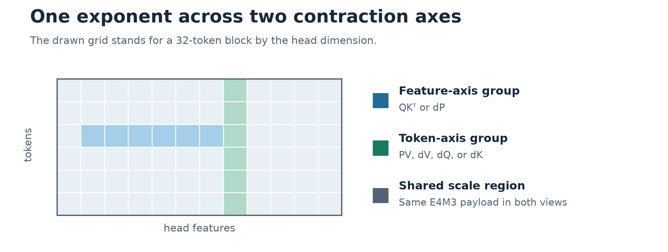
Figure 2. Original schematic from §3.1. A shared exponent covers a whole token block. The horizontal and vertical strips show two hardware group orientations within that region. A smaller scale stripe would usually need fresh rounding for the second orientation.

To see why separate stripes are costly, imagine $X$ stored in BF16 at two bytes per entry. The codes for two independent E4M3 representations already cost two bytes per entry before scales, and conversion can read the BF16 source twice. Sharing the E4M3 payload cuts one code write and, for saved $Q,K,V$, one saved representation. The byte count is illustrative. Layout padding, metadata replication, input rereads under fusion and cache hits affect the actual traffic. Coarser scaling can also increase the influence of a single outlier. The choice buys reuse by giving up resolution in some groups.

Factoring the scales out of the score MMA

The head dimension is special because the scale does not vary across it. In the MXFP8 path, using stored Q/K codes $q^c,k^c$ and their respective token-block exponents gives

$$\begin{aligned} \widetilde S_{ij} &=\alpha\sum_{t=1}^{d} (2^{e_Q(i)}q^c_{it})(2^{e_K(j)}k^c_{jt})\\ &=\bigl(\alpha\,2^{e_Q(i)}\bigr)2^{e_K(j)} \sum_{t=1}^{d}q^c_{it}k^c_{jt}. \end{aligned}$$

Thus the paper can issue an unscaled E4M3 MMA and apply a row and column factor at the score processing stage. The factors still affect the logits supplied to softmax. Pulling them outside the reduction is valid in real arithmetic. The order of floating-point operations and range of intermediate values determine bitwise behavior. NVFP4 uses a finer per-token, per-16-feature scale in $QK^\top$, so this factorization does not apply across the entire feature reduction of that route.

Rotation, range, and the alternative

With an orthogonal normalized Hadamard matrix $H$, one can rotate the last dimension before rounding. The exact score satisfies

$$(QH)(KH)^\top=QHH^\top K^\top=QK^\top.$$

An isolated outlier of magnitude $a$ in one feature turns into magnitudes $|a|/\sqrt d$ across all features in the simplest case. That can help a single coarse scale set by the largest entry. It can hurt per-16 scaling by spreading a previously localized outlier to every group. Appendix A.2 gives an example where the NVFP4 output cosine drops from 0.937 to 0.857 with outlier channels in K, while an MXFP4 comparison rises from 0.749 to 0.816. The authors report no training difference beyond run-to-run noise for their tested routes. The default at $d=128$ is a pragmatic shared choice. Channel mixing within a token does not itself consult future positions.

The straightforward alternative is two fine-scale views. It keeps better local range at the cost of quantization, writes, retained bytes and layout handling. A per-tensor scale has cheap metadata but couples distant tokens and documents. A per-token scale isolates positions but can sacrifice the simple two-axis reuse contract when used in a token-axis MMA. These choices expose the main design trade-off. A scale group is both a numerical approximation and a dependency boundary.

4. A causal mask must include scale selection

A two-token counterexample

Take two scalar values $v_1=1$ and $v_2=a$. Query 1 sees only key 1, so its exact attention output is $1$. For a deliberately simple signed quantizer use the code set $\{-2,-1,0,1,2\}$ and the shared scale $s=\max(1,|a|)/2$. Reconstruct $v_1$ as $s\operatorname{round}(1/s)$. When $a=2$, the scale is 1 and the reconstructed value is 1. When $a=6$, the scale is 3 and the reconstructed value is 0. The query never multiplies by $v_2$. It still reads a rounded value that $v_2$ helped choose.

$$\widetilde O_1(a)= \underbrace{\widetilde P_{11}}_{1}\, s(a)\operatorname{round}\!\left(\frac{1}{s(a)}\right).$$

This is an illustrative integer quantizer, separate from the paper’s FP4 format. The FLAMIA scenario uses a scale shared by keys in a tile. Fully visible tiles can use group scales since every key in the group is in the prefix. A diagonal tile contains the frontier between visible and invisible keys. Some groups straddle that frontier and allow the same mechanism as the example.

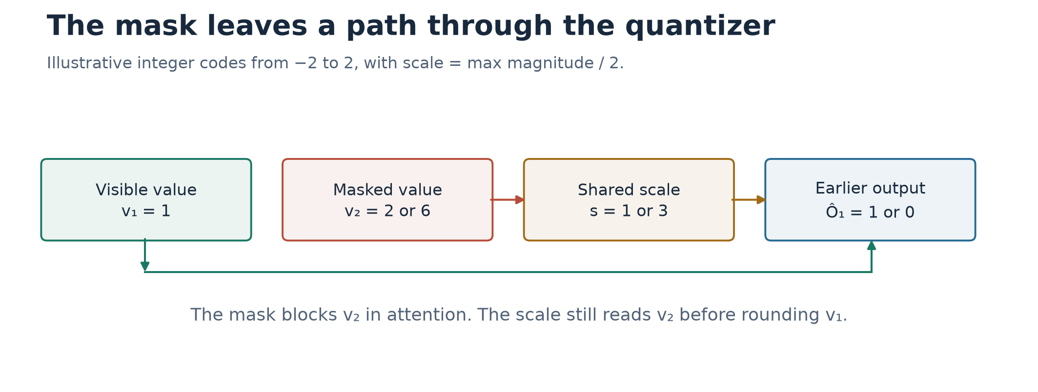
Figure 3. Original schematic and arithmetic example motivated by paper Fig. 1. Future value growth changes the shared scale from 1 to 3. Query 1 consumes a different reconstruction of value 1 while its mask stays fixed.

Why doubling the scale often preserves E4M3 values

Suppose the code for $x/s$ is a normal E4M3 number and the corresponding code at $x/(2s)$ remains normal, away from clipping. Doubling $s$ shifts the exponent of the unrounded code down by one. A corresponding code and its neighbors halve, so round-to-nearest ordinarily selects a code half as large, including consistent tie handling under this lattice shift. Multiplication by the new scale gives the same represented value. At the subnormal boundary the lattice no longer halves with the exponent. For example, in the standard E4M3 lattice the smallest subnormal code has magnitude $2^{-9}$. A value already represented by that code with scale $s$ is halfway between zero and the smallest subnormal at scale $2s$. Its reconstructed magnitude changes under either tie choice.

Clipping gives a second failure. Let $a=\max_{u\in b}|X_u|>0$ and let the maximum finite E4M3 code have magnitude 448. The conservative scale follows from $a/2^{e_b}\le448$.

$$e_b \ge \log_2(a/448),\qquad e_b=\left\lceil\log_2(a/448)\right\rceil$$

This is the smallest power-of-two exponent satisfying the inequality when the scale format can represent it. Zero blocks can use a conventional finite scale. A floor rule based only on the largest code exponent can allow $a/2^{e_b}$ to exceed 448. As a concrete example, $a=480$ at scale 1 clips to 448. At scale 2 its target code is 240, which is representable, and its reconstructed value can be 480. Upward rounding prevents that saturation mechanism but leaves the subnormal boundary. Operand groups can couple positions within their own 32-token block. The tiled $dS$ scale has an analogous dependency between rows.

Folding a local scale into the companion operand

Let $s_j$ be a scale determined by key position $j$ alone and let $v^c_j$ be its stored code vector. The contribution of that key to a query is

$$P_{ij}\widetilde V_j=P_{ij}(s_jv^c_j) =(P_{ij}s_j)v^c_j .$$

For the 4-bit V case, this moves the per-key factor into the probability operand on diagonal tiles. Visible probabilities carry their own key’s scale, and masked keys contribute zero. The same algebra moves the key-local factor for $dQ$ from $K_j$ into the corresponding $dS_{ij}$ term, which the paper calls K fold. The key-side $dP$ contribution needs compatible per-key V scaling as well. Quantization after the fold can change error and range, so algebraic equivalence does not imply bitwise equality. Applying the fold everywhere costs work that cannot improve prefix isolation on already fully visible groups. At 32,768 tokens the paper reports 1.04 times forward latency for diagonal-only per-key V scaling and 2.83 times for doing it on every tile in that ablation.

Forward locality and backward locality differ

FP16 reduces the write traffic of partial $dQ$ at the cost of a five-bit exponent field. The kernel boosts partials with a power-of-two scale before accumulating them and inverts the scale afterward. Suppose $a_i$ is a conservative size estimate for a row’s partials and $h$ is a safe representable target with headroom. A stylized choice is $2^{\lfloor\log_2(h/a_i)\rfloor}$. In real arithmetic the prescale cancels. Round-off inside FP16 depends on the prescale, so a sequence-wide estimate transmits a suffix outlier to earlier query rows even when the keys being reduced are all visible. Appendix A.4 reports a maximum observed change of up to $5\times10^{-4}$ relative to the largest entry under its probe.

For fixed incoming $G_i$, the exact formula for $dQ_i$ needs $Q_i$ and prefix K/V. To respect that dependency, the causal accumulator scale combines $\|G_i\|$ with running maxima of key and value magnitudes through $i$. The expected prefix invariant for $dQ_i$ is conditional on $G_i$ being held fixed. $dK_j$ and $dV_j$ legitimately receive gradient contributions from queries after $j$, so the same invariant is inappropriate for those full reductions. The strict options also use per-token operand scales and a per-query-row $dS$ scale. Packed documents, windows, and all-4-bit backward still use the default accumulator scale in this paper. Document-local input quantization and strict backward locality are distinct guarantees.

5. Reconstructing the forward in the backward

An error decomposition for the centering term

Let $p'$ denote the backward’s reconstructed probability row, $E'$ its value-gradient product, and $D'$ the scalar calculated from the saved forward output and reconstructed incoming gradient. Let $r=\sum_j p'_j$ be its mass and $D^\star=\sum_j p'_j E'_j$ its own weighted sum. The row sum before quantizing $dS$ becomes

$$\begin{aligned} \sum_j p'_j(E'_j-D') &=D^\star-rD'\\ &=(D^\star-D')+(1-r)D'. \end{aligned}$$

The first difference includes changed operands, a changed exponential or tile policy, and rounding in the stored output. The second term isolates the failure of the probability row to sum to one. A common reconstructed $G$ and $V$ removes one cause of the first discrepancy. A correction that centers the row with $D^\star/r$ would enforce a zero row sum for $r>0$ in exact arithmetic on the reconstructed values. It would require gathering the row’s weighted sum and mass before the gradient products. That changes the approximation and the fused schedule. This is a diagnostic alternative derived here. FLAMIA uses the cheaper $G'\cdot O$ path and aligns its numerical inputs with $E'$.

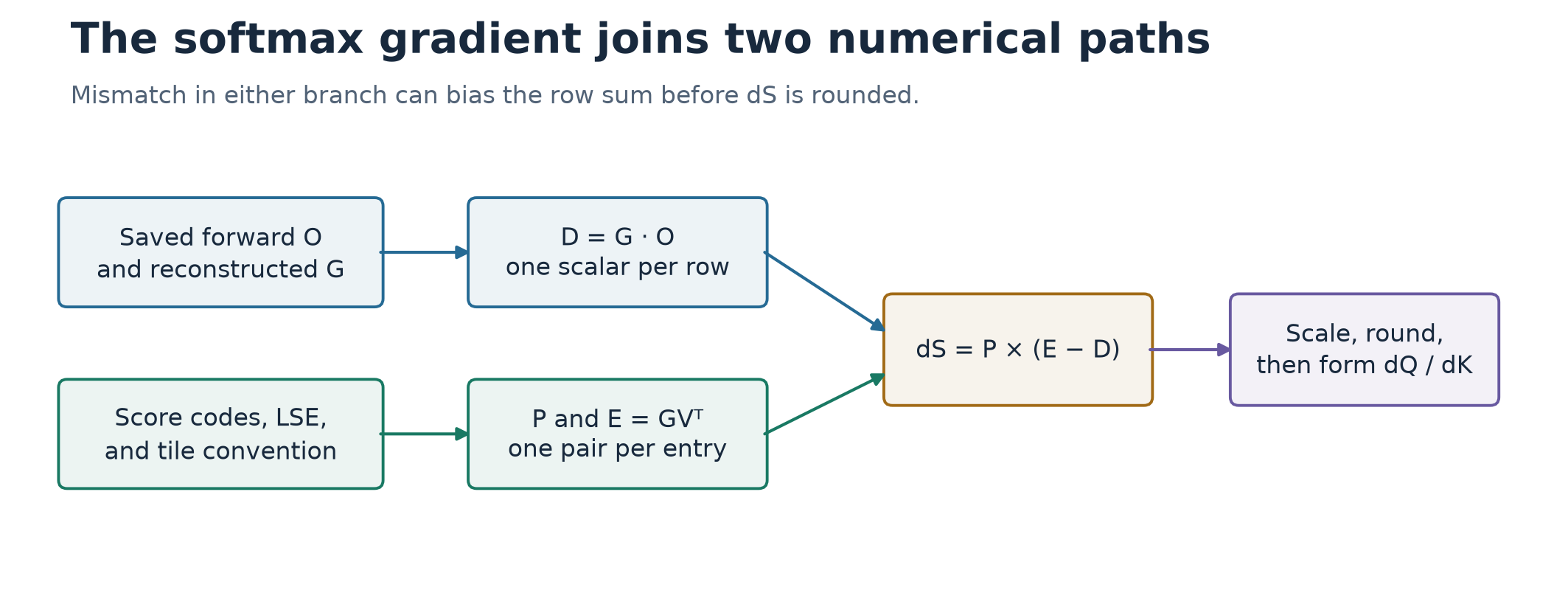
Figure 4. Original schematic based on paper §3.3. The saved output feeds the row scalar, while the reconstructed score and LSE feed the probability tile. A mismatch at either branch can bias the product.

What should “same” mean in a fused GPU kernel? Using the same Q/K codes is necessary to reconstruct the score path, but consistent exponent evaluation and diagonal tile decisions matter as well. Different tile boundaries can change whether a tile uses a fold and can change intermediate maximum choices. The saved LSE defines the normalizer the backward thinks it is using. A tile formed with a different approximation can combine with that normalizer to give a different row mass even when absolute score changes look small.

Algorithm 1. Microscaled forward and recomputed backward

This numbered pseudocode abstracts the default numerical route from §§3.1–3.5. It omits warp instructions, separates semantic operations that the kernels fuse, and makes the strict settings explicit. The all-4-bit experimental path is outside the default route.

01  Choose MXFP8 or mixed NVFP4/FP8 and a scale policy.
02  Rotate Q and K per token if enabled; form score codes.
03  Form E4M3 V and gradient Q/K views; share views when legal.
04  For each valid query tile, initialize online row state.
05    For each visible key tile, reconstruct scaled logits.
06      Apply document and causal masks; update row state.
07      Round scaled weights; add their value contribution.
08    Save normalized BF16 O and row LSE for backward.
09  Encode G once; compute D from reconstructed G and saved O.
10  Select sequence-wide or causal row dQ accumulator boosts.
11  For each eligible backward tile, reconstruct the same logits.
12    Rebuild P with saved LSE and matching numerical rules.
13    Form E = G times transpose(V) using matching views.
14    Form U = P * (E - D); quantize U at the chosen granularity.
15    Accumulate dV, dK, and boosted FP16 dQ partials.
16  Undo the dQ boosts; return BF16 outputs and gradients.

The forward probability operand is tied to the online numerator and its scaling. The backward uses saved row statistics for normalized reconstruction. Their scaling and layouts can differ by product, while their conventions for building the underlying weights must agree. This is the same strategy that allows the output gradients to stay BF16 and $dS$ to be quantized inside the attention kernel. The paper’s matched route is still a chosen approximate gradient. It does not differentiate the finite quantization map exactly, whose rounding operation is discontinuous.

A range budget for probability quantization

In base-2 softmax, suppose the retained row reference $m$ can lag the current maximum by $\tau$. The largest exponent argument is at most $\tau$, so unnormalized weights satisfy $w\le2^\tau$. Let $2^c$ boost small weights before rounding and be removed after the MMA. Avoiding saturation requires

$$2^c w\le2^{c+\tau}\le448 \quad\Longrightarrow\quad c+\tau\le\log_2(448)\approx8.81 .$$

The default MXFP8 pair $(c,\tau)=(4,4)$ gives a bound of 256. A tempting pair $(8,2)$ admits 1024, which clips to 448 before accumulation. The final division by $2^8$ does not undo clipping. At that endpoint the reconstructed weight is $448/256=1.75$ rather than 4. An exact running maximum allows a larger boost, but earlier tiles need to be rescaled more often. Appendix B.1 gives the comparison with $(8,0)$ and notes a boost of $2^8$ for the probability operand in the backward’s $dV$ product. I would keep the parameters coupled in a benchmark report. The same $c$ means different numerical headroom under a different maximum-retention policy.

Small gradients deserve a metric of their own

The entries of $U$ mix a softmax factor, often tiny, with a centered dot product. When the scale covers a larger maximum, many entries cross the zero-rounding threshold together. A global norm can still look good because those entries carry little squared mass. An illustrative vector has one entry equal to 1 and 100 equal to 0.001. Dropping the 100 entries yields a relative Euclidean error of about 1% and a cosine of about 0.99995, while 100 of 101 nonzero entries are gone. That example shows what a cosine can miss. It says nothing about the task utility of any particular gradient coordinate. The paper’s 32 by 32 maxima restore more gradient entries and allow two-axis reuse. Per-row scales may improve locality, while finer 2D groups or higher precision would shift the cost to extra reductions, data or MMA work.

6. Packed documents and GPU scheduling

Preserve the logical row before optimizing the physical tile

A batch row can contain multiple documents at arbitrary token offsets. In packed causal attention $\Omega_i$ ends at $i$ and starts at that token’s document boundary. This changes both the dense semantics and the number of active tiles. A quantizer that only clips the attention mask can still couple unrelated documents through its scale statistics. FLAMIA defines its token blocks locally to each document and keeps dense per-token scale metadata. The load warp constructs a 128 by 4 scale-factor atom in shared memory when needed. This lets the document start unaligned in the physical buffer while keeping its scale groups tied to its own tokens.

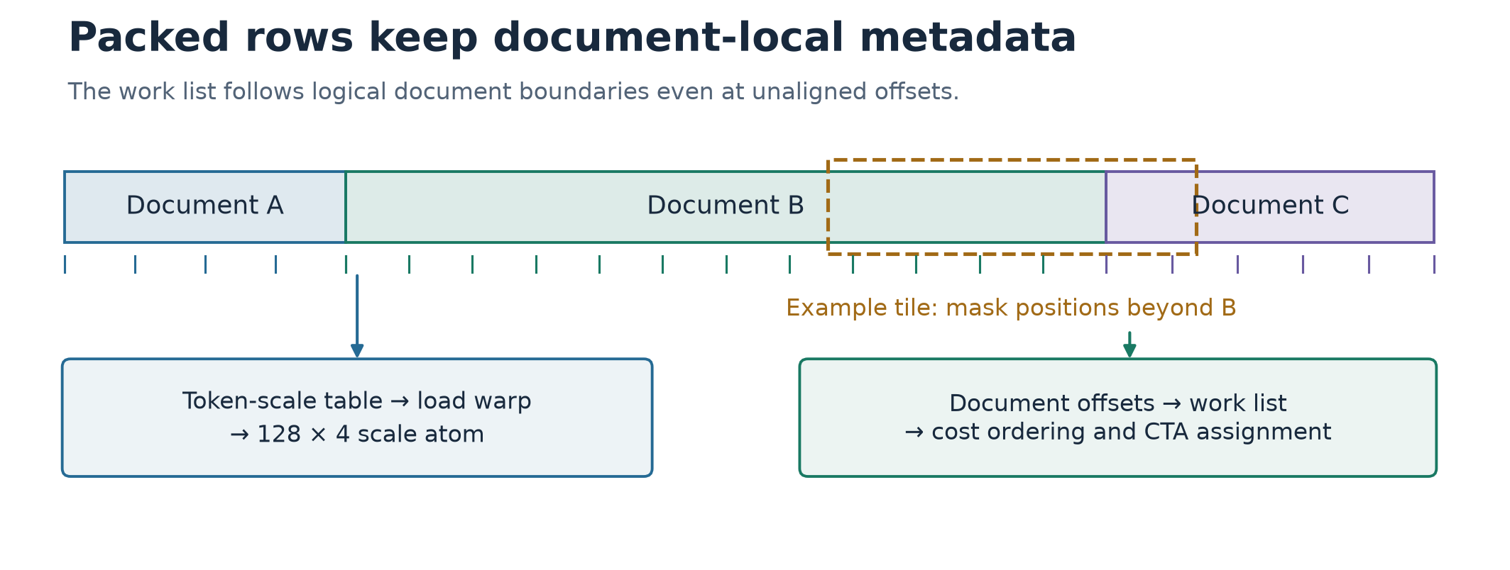
Figure 5. Original schematic based on paper Fig. 2 and §3.6. Logical documents share storage. Per-token scale metadata feeds the loader, while document boundaries and query ranges determine the work list.

Invalid query rows are given an infinite log-sum-exp sentinel so the reconstructed contribution vanishes. Invalid keys inside a partially filled tile are masked. The packing scheme avoids physically repacking every Q/K/V and gradient buffer around alignment boundaries, and it keeps row capacity independent of the current document-length distribution for graph capture. The all-4-bit route has another constraint. The transposed V representation packs two keys per byte. When a document starts at an odd key, a tile would begin on a half byte. Appendix B.2 describes two copies with staggered pairing. Choosing the right copy trades a write once per input for avoiding a nibble shuffle on every loaded tile. This is a cost of the experimental route with 4-bit V.

Cost-based scheduling and tail behavior

For an ideal causal document of length $n$, the number of visible query-key pairs is $n(n+1)/2$. Across packed documents of lengths $n_1,\dots,n_M$ with total length $T$,

$$C_{\rm visible} =\tfrac12\sum_{j=1}^{M}n_j(n_j+1) =\tfrac12\left(T+\sum_{j=1}^{M}n_j^2\right).$$

At fixed $T$, the sum of squares explains why a long outlier document can dominate the call. For example, sixteen 4096-token documents and one 8192-token document plus 224 documents of length 256 both total 65,536 tokens. The former has 134,250,496 visible pairs and the latter 40,927,232. The latter can use less arithmetic overall while putting more work into the tail of a few items. The tile cost also depends on rounding to tile sizes and the causal frontier. TFLOP/s and latency answer different questions here.

Algorithm 2. Document-local work list and launch

This reconstruction from §3.6 and Appendix B.6 emphasizes scheduling semantics. Cost is an estimate in key blocks, excluding pipeline and contention effects.

01  Read document offsets, lengths and query-head groups.
02  Compute token-block scales within each document.
03  Emit work items of up to 256 queries from one document.
04  For each item, estimate the number of visible key blocks.
05  Sort items across the packed row by decreasing cost.
06  Use alternating static assignment across persistent CTAs.
07  In causal calls, permit dynamic CLC work acquisition.
08  In noncausal calls, use CLC when max length >= 4 * mean.
09  Request the next item after the current item's last K/V load.
10  Gather scale atoms and mask keys outside the document.
11  Write O and gradients into their original packed offsets.
12  Order backward key tiles by cost; group heads for L2 reuse.

A cooperative thread array (CTA) is a GPU thread block. Cluster Launch Control (CLC) lets work be picked up dynamically. The acquisition timing matters because reserving work too early can leave otherwise idle CTAs without access to it. Sorting only within each input sequence can still leave a final long item near the tail. A host-side plan adds a CPU interaction on changing workloads. GPU list construction avoids host synchronization and is reused within the microbatch. For backward the paper caps the primary launch and handles overflow persistently, which reduces register pressure compared with putting all descriptor state inside one persistent loop in their tests.

The ≥4 skew rule for noncausal inputs is empirical. A partition dominated by tiny documents can be metadata- and launch-bound even when the visible-pair count is small. One massive document can leave a few long work items that dynamic acquisition cannot split. A runtime model that estimates time from tile count alone may miss GQA head sharing, causal occupancy, and memory locality. Those boundaries are where static and dynamic policies can exchange their ranking.

7. The critical path moves away from the tensor cores

Softmax and TMEM resources

A 128 by 128 score tile requires 16,384 exponentials in the unmasked case. The paper gives 16 and 32 exponentials per clock per SM on the B200 and B300 MUFU pipelines, respectively. Dividing yields 1024 and 512 ideal issue cycles for that count. These are estimates for one operation class before overlap or masking, not measured kernel durations. Offloading some exponentials to polynomial FMAs balances execution pipelines on B200. B300’s faster MUFU can make emulation overhead for the E4M3 path, and the paper disables it there. The forward interleaves the two 64-key halves of the next $QK^\top$ with the current $PV$ to overlap work. On B300 a fused TMEM load and row-maximum reduction is available on fully unmasked tiles.

The log-domain probability path uses the monotonicity of $2^x$. If an exponent-group scale is $2^{e}$, then normalizing the values before quantization can be done in the exponent:

$$\max_j 2^{x_j}=2^{\max_j x_j}, \qquad 2^{x_j}/2^e=2^{x_j-e}.$$

The group maximum can be found before the exponentials and an elementwise division avoided. The §3.5.2 optimization is described for the NVFP4 path. The two default paths still use E4M3 probabilities, and the all-4-bit inference experiment separately uses a 4-bit probability operand. Naming the path by its score format hides this distinction.

On the backward side, two CTAs share operands and can cover 256 keys over a query range. The BF16 accumulator arrangement already fills all 512 TMEM columns at the issue of $dP$. Factoring token scales out of that product frees the design from needing those scale operands in TMEM. For $E_{ij}$ the reconstructed product is $(s_G(i)s_V(j))\sum_k g^c_{ik}v^c_{jk}$. Compute warps can apply those factors after the feature-axis MMA. The FP16 partial reduction then relieves traffic, with data-dependent prescaling to preserve range. Appendix B.3 chooses the two-CTA route by shape and format and keeps deterministic calls on one CTA. Appendix B.5 reports deterministic backward costs of 5–12% for MHA and 20–34% for GQA. Bitwise repeatability and prefix locality should be evaluated separately.

Why inference can tolerate a different approximation

Write $x=n+f$, with $n=\lfloor x\rfloor$ and $f\in[0,1)$. A float’s exponent can carry $n$ and its significand can carry the linear factor $1+f$. The approximation is the secant interpolant of $2^f$ on this interval.

$$2^x=2^n 2^f,\qquad \widetilde w=2^n(1+f),\qquad \frac{\widetilde w}{2^x}=\frac{1+f}{2^f}.$$

Convexity gives $\widetilde w\ge2^x$ before the bias offset. At $f=1/2$, the unshifted relative error is $1.5/\sqrt2-1\approx6.07\%$. Appendix C’s Mitchell-P uses an offset and guarded bit operations, then rounds to E2M1. Coarse rounding bins absorb many small errors, but inputs close to bin boundaries still change codes. The Schraudolph route produces a shifted BF16 approximation, used for five of eight exponential pairs in the reported variant. Small value errors may matter more for E4M3 because its codes are closer together. Zero mean error over a fractional interval would not by itself imply unbiased normalized probabilities on arbitrary, nonuniform score distributions.

The authors report 39.6 nats of maximum within-row range on Gaussian inputs and 386–1653 nats on trained-model captures in their diagnostic. The difference motivates checking bit-pattern clamping and argument domains on real activations, especially if an approximation sees shifted rather than raw logits. The claimed approximation window concerns the arguments after the relevant scaling. I would avoid applying a raw score-range claim directly to a bit-field wrap boundary without checking that unit conversion.

8. What the experiments establish

Time the training call and label the kernel-only comparison

Table 1 times the forward and backward attention call including quantization for packed causal inputs, with 16 query heads and $d=128$. Most rows are MHA and one 16k row is GQA 16/4. The baseline is the fastest supported competitor for each workload. MXFP8 gives 1.10–1.40 times speedup on B200 and 1.06–1.42 times on B300. The 8192 + 224 × 256 shape accounts for the upper endpoint on both GPUs. Its B300 result is 1.67 ms against 2.37 ms for BF16 FA4, a ratio of about 1.42. The cuDNN FP8 value is 2.81 ms and should not be used as that row’s denominator. On B300 with 16 × 4096, the MXFP8 and fastest baseline values are 3.17 and 3.35 ms, yielding about 1.06. The same kernel family gives different advantages depending on the shape.

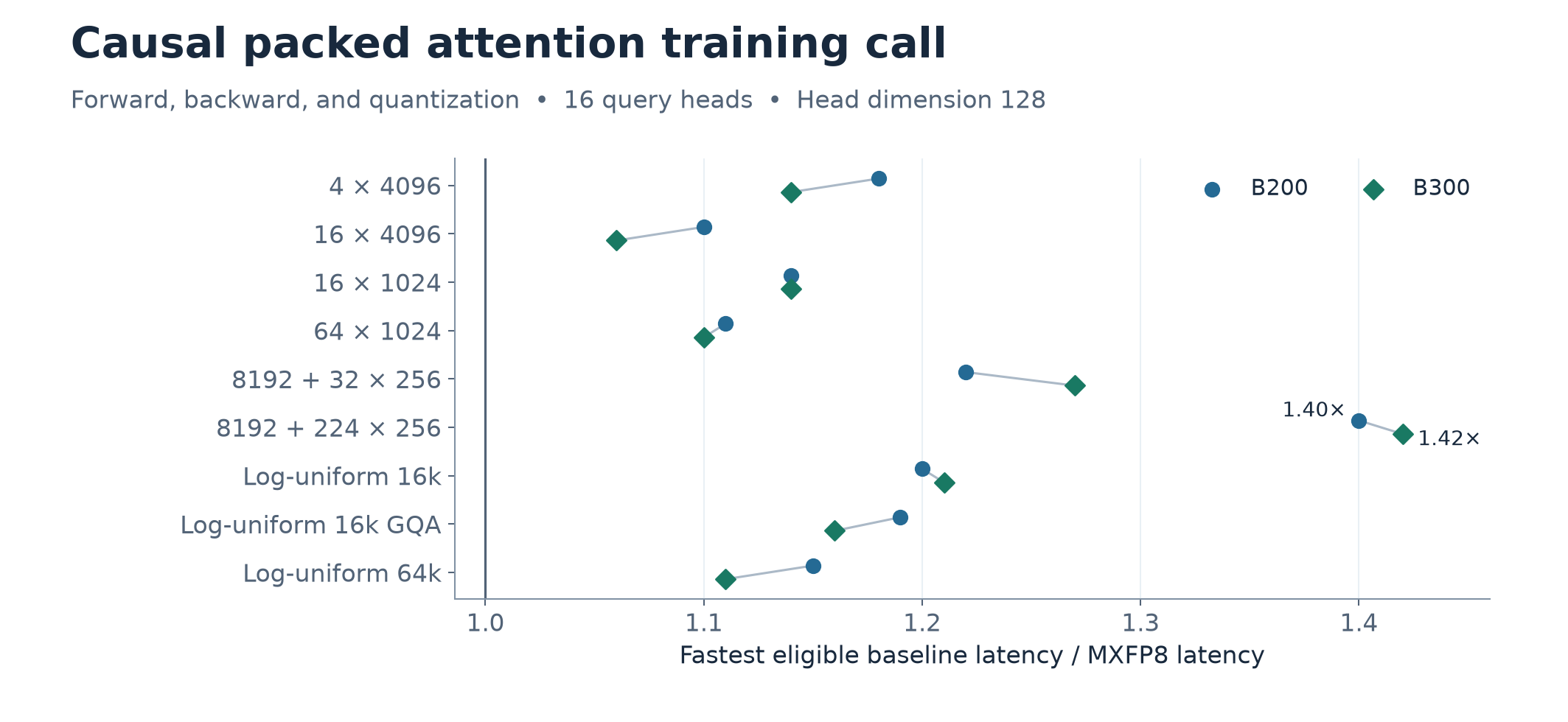
Figure 6. Redrawn from paper Table 1 using its printed ratios. The shape with many short documents and one long one has the highest speedup. The plot compares complete attention calls, including quantization.

Appendix D.1 reports medians of three paired rounds, each captured in a CUDA graph, after warm-up. cuDNN FP8 input scales are computed inside the timed training call, while output scales are calibrated ahead of time using the same data. Some baselines only support the packed forward or do not support causal GQA, so their absence from a backward column is a support boundary. It does not demonstrate that their unsupported modes would be slower. The authors use 128-aligned document starts for FLAMIA’s kernel-only timing. Subtracting the numbers in Tables 2 and 3 from Table 1 would mix layouts, timing scopes and, in some rows, different kernels.

Packed noncausal results in Appendix H have weaker margins. MXFP8 leads all nine B200 training-call rows, while B300 includes ties at displayed precision and small losses. In Appendix J’s batched B300 2 × 8192 noncausal case, MXFP8 takes 2.17 ms and cuDNN FP8 with fresh inputs takes 1.89 ms. The main packed result therefore does not establish a general B300 lead. Baseline calibration also matters. Across 30 packed and batched shapes, the paper reports a median advantage of 7.4% against cuDNN FP8 with all scales precalibrated, 10.3% with fresh input scales, and 112% when a second attention pass is needed to obtain fresh output scales.

Where the saved time goes

The authors report reductions from 789 to 261 microseconds for MXFP8 quantization preprocessing and 640 to 110 microseconds for the NVFP4 preprocessing case at 4 × 4096. Those are measurements of fusion ablations. Removing exponentials altogether leads to a faster diagnostic that cannot compute valid attention. The resulting 45% estimate cannot be interpreted as an independently additive fraction of the original duration. Changes to a component can change overlap with the rest of the kernel.

The mixed route leads the packed causal kernel-only backward results, even though MXFP8 wins the complete training calls. The narrower score operands help recomputation, whereas the remaining backward products stay in E4M3. The mixed backward geometric-mean throughput is 1329 TFLOP/s, versus 571 for all-4-bit and 1015 for BF16 in §4.3. Six separately quantized copies take 45–52% of the all-4-bit backward time there. These numbers explain why the lower peak bit width does not imply better throughput for the whole step.

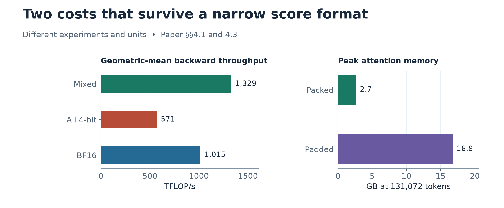
Figure 7. Redrawn from paper §§4.1 and 4.3. Left, geometric-mean backward throughput by route in the ablation. Right, per-call peak memory at 131,072 tokens in the packed and aligned padded cases. The panels use distinct experiments and units.

The authors report 2.7 GB of peak memory for a packed attention call versus 16.8 GB with aligned, padded buffers at $T=131{,}072$. The ratio is about 6.22 using the rounded values. This measures per-call peak memory and depends on the padding construction. At 16k and 64k they also give whole-model training throughputs on one B200, 84.6k and 96.8k tokens/s with packing versus 68.8k and 84.3k with padding. Those comparisons measure layout and padding effects together. To translate a kernel speedup $s$ to an idealized step speedup, let $f$ be the original step fraction spent in that call and assume everything else stays fixed.

$$s_{\rm step}=\frac{1}{1-f+f/s}.$$

At $f=0.30$ and $s=1.42$ this gives about 1.097. Those are illustrative inputs, and a different layout can change both $f$ and the rest of the step. The paper’s Table 1 has no measurement of $f$.

Separate numerical closeness, invariance, and training quality

Table 4 compares FP32-reference outputs and gradients from the same BF16 inputs. On 4 × 4096 causal inputs, MXFP8 reports $O/dQ$ cosine 0.9988/0.9979, mixed NVFP4/FP8 0.9920/0.9906, and all-4-bit 0.9810/0.9456. The exact causal probe in Table 5 is a different experiment. Its suffix perturbation changes the scale group maximum. The exact options with causal $dQ$ scale give observed zero change in the reported $O$ and $dQ$ probes. The floor-exponent cuDNN MXFP8 case reports 0.11 for both relative changes. The default cuDNN MXFP8 values are much smaller at $6.9\times10^{-6}$ and $1.1\times10^{-5}$. These rows should be read as measured maxima under the chosen perturbation, not universal error bounds.

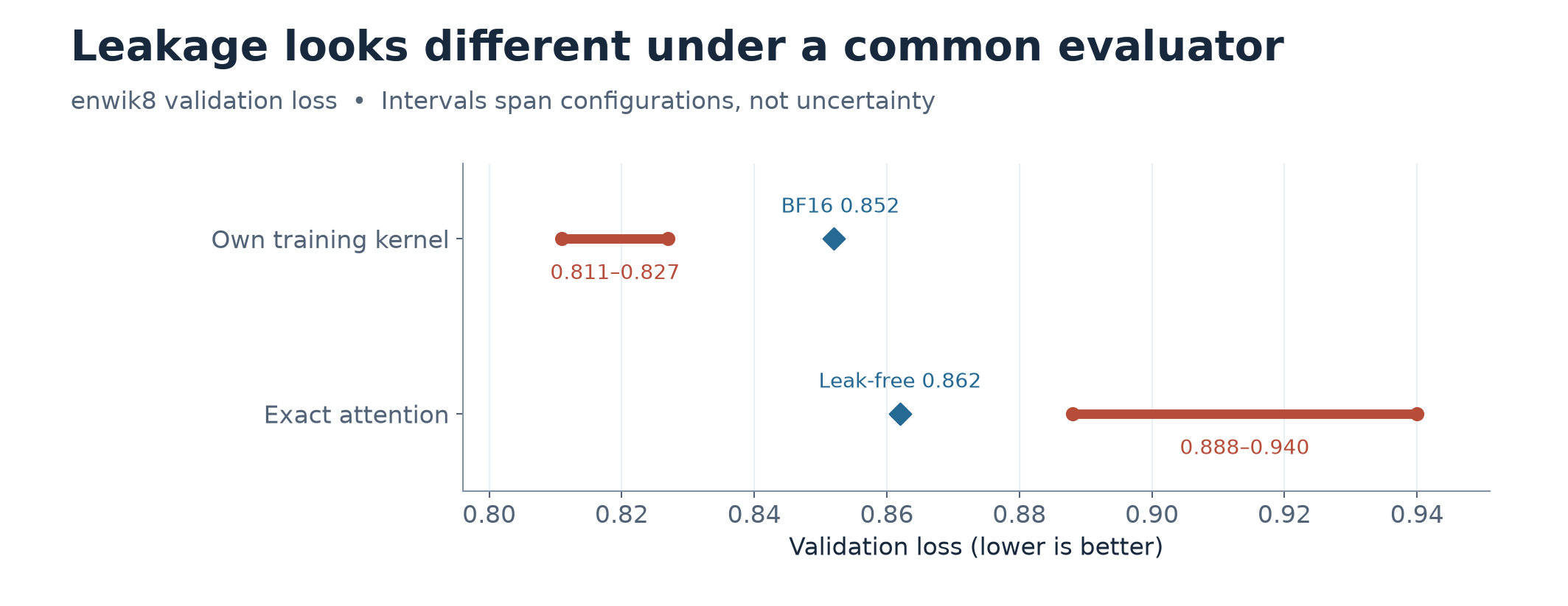
Figure 8. Redrawn from §4.5. The intervals span the reported leaking configurations in each evaluation mode. Endpoints are ranges across configurations rather than confidence intervals. The BF16 and leak-free reference points are reported separately.

In the six-layer, width-1024 enwik8 experiment, the leaking 4-bit setups report 0.811–0.827 validation loss when evaluated through their own kernel, compared with 0.852 for BF16. Exact attention applied to the leaking checkpoints gives 0.888–0.940, compared with 0.862 for a model trained without the leak. A change in validation kernel can reverse the impression created by the lower loss. The range endpoints do not identify which checkpoint produced which pair of numbers, so the plot does not draw pairwise connectors.

The same section reports divergence within 500 steps when different incoming-gradient representations feed $D$ and $dP$, and divergence by step 500 when exponentials are approximated only in the forward. Using 256-query diagonal handling forward and 128-query handling backward drives gradient norm from 0.5 to $2\times10^5$ despite an initial $dQ$ cosine of 0.945. In the $dS$ ablation, the share rounded to zero rises from 0.4% to 29% and the validation gap to BF16 rises from 0.0008 to 0.049. The paper reports similar norm error across the compared choices. This is evidence that the error distribution matters. The scale intervention changes multiple properties at once, so the comparison does not establish the causal effect of zeroing by itself.

The 1B pretraining results

Table 6 gives the final 1000-step mean training loss and five final-checkpoint evaluation scores. The model is Llama-3 style, 1B parameters, 2k-token contexts, trained on roughly 100B FineWeb-Edu tokens with eight B300 GPUs. Appendix G lists AdamW, global batch $2^{20}$ tokens, 100,000 steps, peak learning rate $3\times10^{-4}$ and 300 warmup steps before linear decay. The nominal batch-step product is approximately 104.9B tokens, consistent with the rounded scale description.

Metric	BF16 FA4	MXFP8	Mixed NVFP4/FP8
Final-window training loss	2.392	2.397	2.406
ARC Challenge	0.3925	0.3618	0.3677
ARC Easy	0.6481	0.6460	0.6557
HellaSwag	0.5711	0.5650	0.5610
PIQA	0.7280	0.7323	0.7258
WinoGrande	0.5762	0.5635	0.5967
Five-task mean	0.5832	0.5737	0.5814

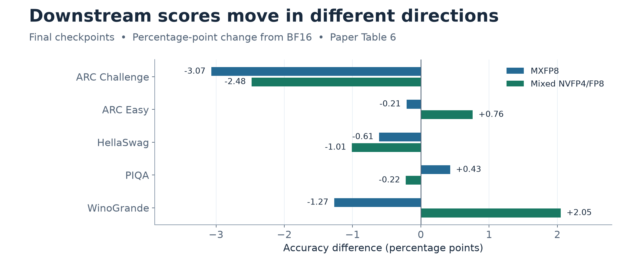
Figure 9. Recomputed differences from paper Table 6 in percentage points. Both low-bit paths lose ground on ARC Challenge. WinoGrande moves in different directions for the two paths.

The MXFP8 loss increase is 0.005 and the mixed increase is 0.014. Their five-task mean changes are −0.95 and −0.18 percentage points using the reported mean row. ARC Challenge drops 3.07 and 2.48 points. WinoGrande moves −1.27 and +2.05 points. A mean close to baseline can reflect offsetting changes. Small loss increases plus mixed benchmark changes support feasibility for this setup. An equivalence claim would require variability estimates and a margin chosen in advance. The mixed path being closer on the mean also does not establish that fewer score bits are better for quality. Final metrics include the effects of two different training trajectories.

9. Reproduction notes and limitations

A comparable latency report should state which of the following it times: quantizer plus both attention passes, standalone forward or backward, or the full model step. Match hardware, document lengths and order, causal mask, head size and GQA ratio. For a baseline needing output scales, record how those scales were obtained. Normalize visible-pair FLOP counts consistently and specify the number of FLOPs counted for a multiply-add. Appendix E notes a benchmark convention with no causal discount, which can nearly double the reported causal throughput for long rows. Compiler version also matters: the authors report changes of roughly 19–21% under a different CuTe DSL version with bitwise-identical outputs. Record the toolchain and retain matched shapes before extrapolating to another environment.

For a numerical comparison, use matched inputs from a trained model and a high-precision reference. Report $O$, $dQ$, $dK$, $dV$, signed row residuals, code underflow, and overflow. Log the scale policy as well as the stored format. Document-local scale calculations, per-token versus token-block scaling, the $dS$ scale, and the $dQ$ accumulator are four distinct choices. Appendix F describes the authors’ TorchTitan integration, selective checkpointing, and graph-capturable operators. Appendix D provides the official resource. The mathematical examples and table differences in this review are derivations and recalculations. Training curves, latency and cosines quoted here are the authors’ measurements.

Several limits follow from the experiments. The strict dependency modes apply to the supported batched causal path. Default packed timing includes residual within-block and accumulator dependencies. The causal $dQ$ scale alone costs 8–11% in the backward and 6–9% in the complete attention call at 32,768 tokens in the reported ablation. This overhead cannot be subtracted from every packed-row speedup because the strict path and the timing workloads differ. Noncausal and batched tables show that the relative ranking can change with layout. The 100B-token run uses 2k-token contexts, so it cannot answer whether quality matches at the very long packed shapes used in the timing suite. The approximate exponentials in Appendix C belong to inference experiments. Mitchell-P reduces latency for some noncausal packed shapes while increasing it on causal ones, where diagonal per-key scaling contributes extra cost. Table 7’s cosine caption uses “Direct-P” where the columns and §4.4 describe Mitchell-P, so I rely on the explicit §4.4 comparison when discussing that accuracy range.

10. Critical analysis

Turn prefix independence into a tested contract

I would define prefix isolation separately for $O$ and for row-local $dQ$ conditioned on fixed upstream gradients. Given any two equal-length inputs that agree through query $i$, change K and V strictly after $i$, and compare the selected prefix outputs. Repeat with different physical document offsets and one fixed set of incoming gradient rows. A deterministic reduction simplifies the bitwise comparison. A separate run with the default atomic reduction should measure repeated-input variance before interpreting small differences. A positive-control suffix perturbation should deliberately cross a scale exponent threshold or the E4M3 subnormal boundary. A negative control should perturb a different document and vary only its physical packing offset. The same suffix test can miss a layout-dependent error if all sampled document starts are aligned.

The missing comparison is a packed result that meets the strict contract. A segmented prefix maximum for each document could supply the row-local accumulator bounds, with per-token operand scales and per-query $dS$ rules for the affected tiles. A two-path design could retain shared-block work where the complete scale group is in the query prefix and pay for finer locality on the boundary. This would require checking all contributing products, including $dS$ and the reduction, so simply changing diagonal V would leave other channels open. The trade-off should be measured with the same packed inputs and the same quantization timing as Table 1. Include cases with many tiny unaligned documents. Those cases increase the ratio of boundary work to fully visible work and are likely to decide whether the proposal pays off.

Isolate gradient-tail effects from gradient bias

A larger $dS$ scale can alter many things at once: zeros, signed bias, saturation and the magnitude of the surviving entries. One intervention would keep the same fine-scale backward and independently zero a matched number of small entries within each tile. Another would hold sparsity approximately fixed while changing the scale and comparing signed residuals, row mass and optimizer moments. Stratify by head, layer, score entropy and token position. For attention rows with a sharp maximum, rare contributions may matter in particular positions even when the mean norm error looks unchanged. These controlled experiments would help explain whether the zero fraction predicts degradation because it removes specific directions or because it tracks another format-induced bias.

The row residual formula in §5 motivates comparing a matched-but-inexact $D$ branch with a centered reference computed directly from reconstructed tile statistics. Such a reference could be slow and still be useful as a diagnostic. A follow-up can report per-row residual quantiles before and after rounding $dS$, along with the measured runtime penalty for centering. It can then test whether the affected rows align with long-run gradient norm spikes. Matching the computation graph is the first intervention. Measuring the error that remains would distinguish ordinary round-off from repeated directional bias.

Measure scheduler and model claims at the right level

The largest packed win combines a skewed workload and a different total of active pairs from the balanced control. An informative sweep would keep token count and $\sum_j n_j^2$ approximately fixed while permuting the document order and changing the tail of the length distribution. Report CTA idle time near completion, schedule build time separately, and repeat for MHA and GQA. Comparing kernel throughput and tokens per second under that design would reveal when the gain comes from useful MMA work and when it comes from less idle time. A baseline with the same work list and BF16 would further separate scheduling from format changes.

For model quality I would pair identical data orders and initialization seeds for BF16, default MXFP8 and strict causal configurations on an accessible batched workload. Evaluate every checkpoint under a common reference attention implementation, then add an evaluation under its own kernel to detect a gap. Include multiple context lengths, downstream score uncertainty and a predeclared equivalence margin. The paper’s leakage experiment shows why comparing only each run’s native validation loss can hide the exact failure the experiment aims to measure. A common reference also makes it possible to distinguish training damage from a transient numerical evaluation difference.

11. Conclusion

FLAMIA changes scale geometry to address two problems together. A shared exponent across a document-local token block can remove duplicate E4M3 payloads and let kernels apply some scales outside the MMA. The same geometry defines how far a suffix perturbation can travel. Per-key folding on a causal boundary and a prefix-sized accumulator boost are consequences of tracing that dependency through the operations, including the backward.

Read the latency and dependency results together. The packed speedup comes from default MXFP8 under the paper’s benchmark conditions. Strict prefix invariance requires separate options with narrower support. These conditions determine which result can be compared with another kernel.

References and reading map

• Velikonivtsev, Koltakov, and Kuznedelev. FLAMIA, arXiv:2611.03344v1. See §§2–3 for design, §4 for experiments, and Appendices A–J for numerical, timing, and shape details. Paper
• Dao et al. FlashAttention, for tiled attention and IO analysis. Paper
• Zadouri et al. FlashAttention-4, for Blackwell scheduling. Paper
• Darvish Rouhani et al. Microscaling Data Formats for Deep Learning, for MX formats. Paper