Polar: Training Native Agent Harnesses Through the Model Boundary

Review date: 2026-11-05
Author: Zhongzhu Zhou
Paper reviewed: Polar: Agentic RL on Any Harness at Scale
Paper authors: Binfeng Xu, Hao Zhang, Shaokun Zhang, Songyang Han, Mingjie Liu, Jian Hu, Shizhe Diao, Zhenghui Jin, Yunheng Zou, Michael Demoret, Jan Kautz, Yi Dong
arXiv: 2605.24220v1
Version and date: v1, 22 May 2026

1. What changes when the harness becomes the environment?

I read Polar as a systems paper about preserving the object we want to train. A coding agent is more than a checkpoint plus a list of tools. Its harness decides how to serialize tool calls, construct prompts, compact context, launch child agents, and decide that a patch is ready. Replacing that machinery with a convenient training loop changes the policy’s environment. A model that learns the replacement interface may still perform poorly inside the product harness.

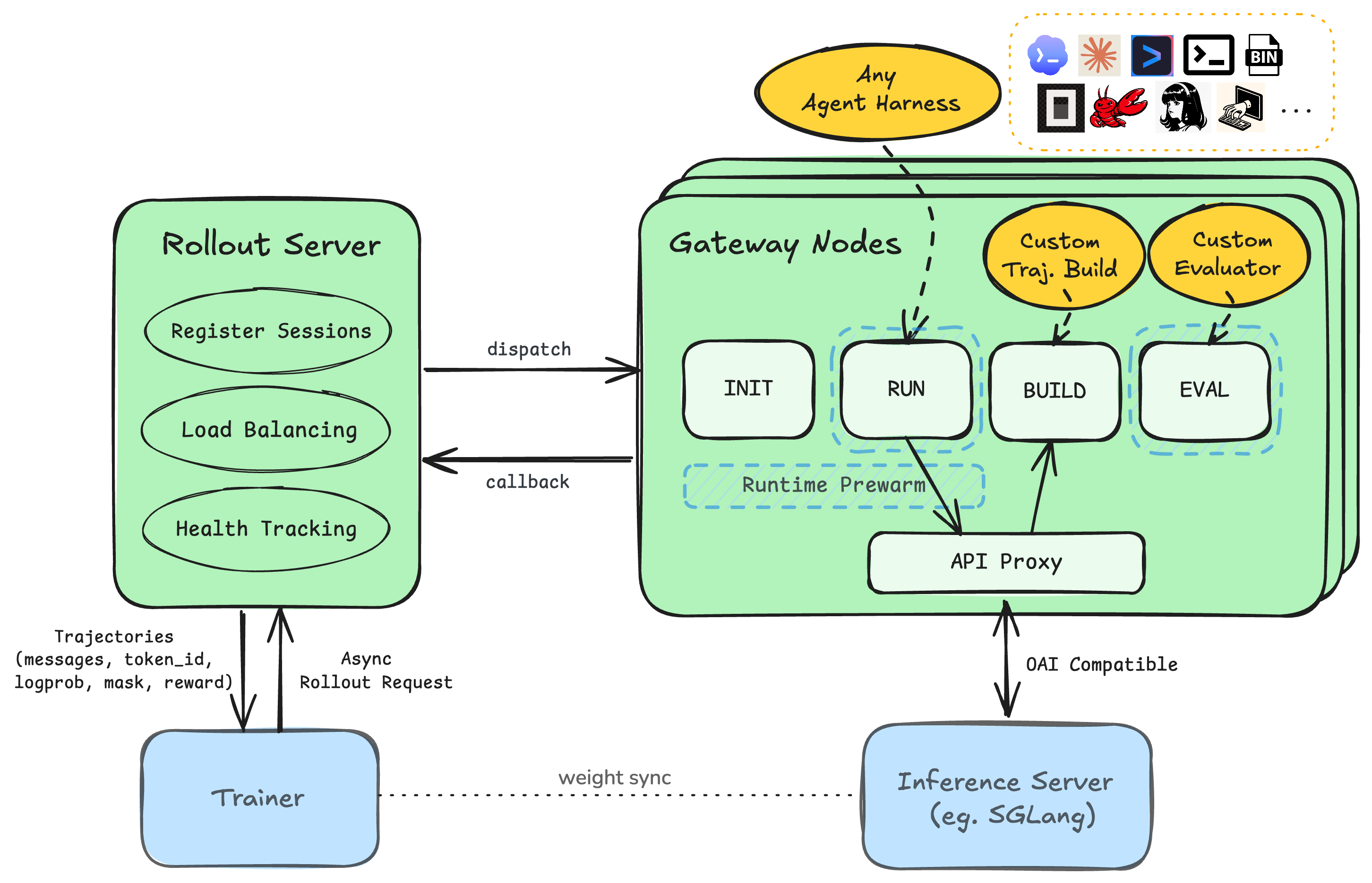
Polar moves the integration boundary to the model endpoint. The native executable runs in an isolated runtime and talks to a provider-compatible proxy. The proxy forwards requests to a local inference service, captures token IDs and behavior log probabilities, and reconstructs samples for an independent trainer. This is useful because many harnesses already allow the model endpoint to be configured, even when their internal event loop is unavailable.

The paper contributes three connected mechanisms: a rollout service with independently scheduled stages; a model API boundary that accommodates several provider protocols; and reconstruction that combines compatible calls while retaining sampled tokens. Its experiments train Qwen3.5-4B through four coding harnesses and demonstrate an offline trajectory-generation workload. Polar extends the earlier ProRL Agent service design; it is distinct from the similarly named ProRL prolonged-reasoning paper.

My central qualification is that there are several meanings of fidelity. Preserving token identities, preserving the conditioning history of those tokens, preserving the harness’s observable behavior, and preserving an optimization objective are different requirements. Polar directly addresses the first and substantially improves the integration story. The other three require additional conditions that deserve explicit treatment.

2. Prerequisites: sessions, policies, and asynchronous work

2.1 A session contains several model calls

A task is a problem instance. A session is one independent attempt at that problem, with its own runtime and deadline. A completion is one model API call inside a session. A reconstructed trace is a trainer-facing sequence assembled from one or more compatible completions. Confusing these units makes both throughput and reward accounting hard to interpret.

Let a completion be $C_i=(p_i,a_i,\ell_i,m_i)$: prompt token IDs, sampled response token IDs, their behavior log probabilities, and structured messages. The model chooses tokens; the harness and environment insert other context. For a token $a_{i,t}$, the relevant conditional distribution is

$$\pi_b(a_{i,t}\mid p_i,a_{i,<t}),\qquad \ell_{i,t}=\log\pi_b(a_{i,t}\mid p_i,a_{i,<t}). \tag{1}$$

The subscript $b$ identifies the behavior policy used during rollout. A later trainer may use different parameters. Keeping the sampled token while attaching the probability of a different token or a different context produces an inconsistent training record.

2.2 Why text is insufficient

Tokenization need not commute with decoding. If $D$ is decoding and $E$ is encoding, a sampled token sequence $a$ need not satisfy $E(D(a))=a$. Several token sequences can render the same text. Tool-call JSON and provider-specific reasoning fields add another layer of normalization. The trainer therefore needs the original sampled IDs, rather than a fresh encoding of a readable transcript.

Environment text has a different role. A test log can influence the next action, but the policy did not generate that log. It should be part of the conditioning context and have zero policy loss. A loss mask distinguishes provenance at token granularity; it does not remove those tokens from the attention context.

2.3 Policy gradients explain the data contract

For a fixed task distribution and a session outcome $R$, the score-function identity gives the familiar policy gradient. Under the assumption that only model actions depend on the parameters being optimized,

$$\begin{aligned} J(\theta)&=\mathbb{E}_{\tau\sim\pi_\theta}[R(\tau)],\\ \nabla J(\theta)&=\mathbb{E}\left[R(\tau) \sum_{i,t}\nabla\log\pi_\theta(a_{i,t}\mid p_i,a_{i,<t})\right]. \end{aligned} \tag{2}$$

This is background reasoning, not an objective newly derived by Polar. It explains why the sampled IDs, their original contexts, and the reward’s unit all matter. It also shows why broadcasting a final reward to actions is not automatically mathematically wrong. A terminal return can weight every action in a Monte Carlo policy gradient. The difficulty is whether the downstream trainer preserves session grouping, relative advantages, and the intended sample weights.

In asynchronous training, a token-level importance ratio has the schematic form

$$\rho_{i,t}(\theta)=\exp\left[ \log\pi_\theta(a_{i,t}\mid p_i,a_{i,<t})-\ell_{i,t}\right]. \tag{3}$$

This expression requires the same action and conditioning event in numerator and denominator. Clipping or truncating ratios may control variance; it cannot repair a denominator associated with the wrong event. The paper lists TIS as enabled but does not provide a full derivation of its trainer-side estimator. I do not infer that estimator from the acronym alone.

3. Why the model API is a useful, imperfect boundary

The gateway recognizes Anthropic Messages, OpenAI Chat Completions, OpenAI Responses, and Google-style requests from paths and headers. It transforms roles, content parts, tool schemas, stop controls, and generation options into the inference backend’s chat format. It also requests training fields such as log probabilities. The returned response is mapped back to the schema expected by the harness.

The adapter’s job is correspondingly small: prepare normal configuration, register tools or skills when needed, and launch the executable. The runtime interface covers start, stop, execution, upload, download and cancellation. Docker and rootless Apptainer are the two backends described in the paper. This separation permits a harness or runtime to change without rewriting the trainer’s optimization loop.

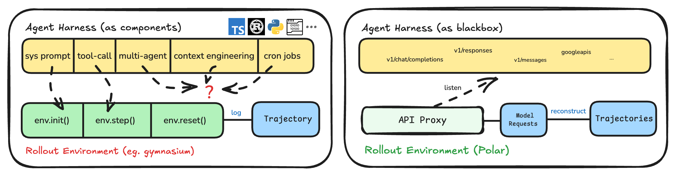
There is an unavoidable tradeoff. A framework-owned environment can expose rich internal state and intermediate rewards, but requires integration with the framework. An API proxy is less intrusive and works across executable boundaries, but can only observe what crosses that endpoint. Hidden model calls that bypass it, internal state changes, and tools that have effects outside the runtime remain outside its direct trace view.

Protocol compatibility also has a temporal dimension. The paper obtains a complete, non-streaming upstream response and emits a synthetic provider-shaped stream. That can satisfy a harness’s event parser while changing time to first token, cancellation behavior, and the interleaving of tool execution with generation. The demonstrated coding workflows support the practical usefulness of the choice. They do not establish behavioral equivalence for agents whose decisions depend on incremental delivery or strict latency budgets.

I would describe the resulting contract as native harness execution with externally mediated model traffic. Saying that every aspect of the original application is unchanged would be stronger than the evidence. The boundary removes a large integration obligation; it does not eliminate the need to state supported provider semantics.

4. Staging the rollout lifecycle

Polar separates durable task management from gateway-local execution. The rollout server expands a task into independent sessions, dispatches them, receives completion callbacks, persists terminal results, and exposes polling. A gateway owns the session runtime, model proxy, reconstruction, evaluation and teardown. Co-locating capture with session ownership simplifies attribution of model calls.

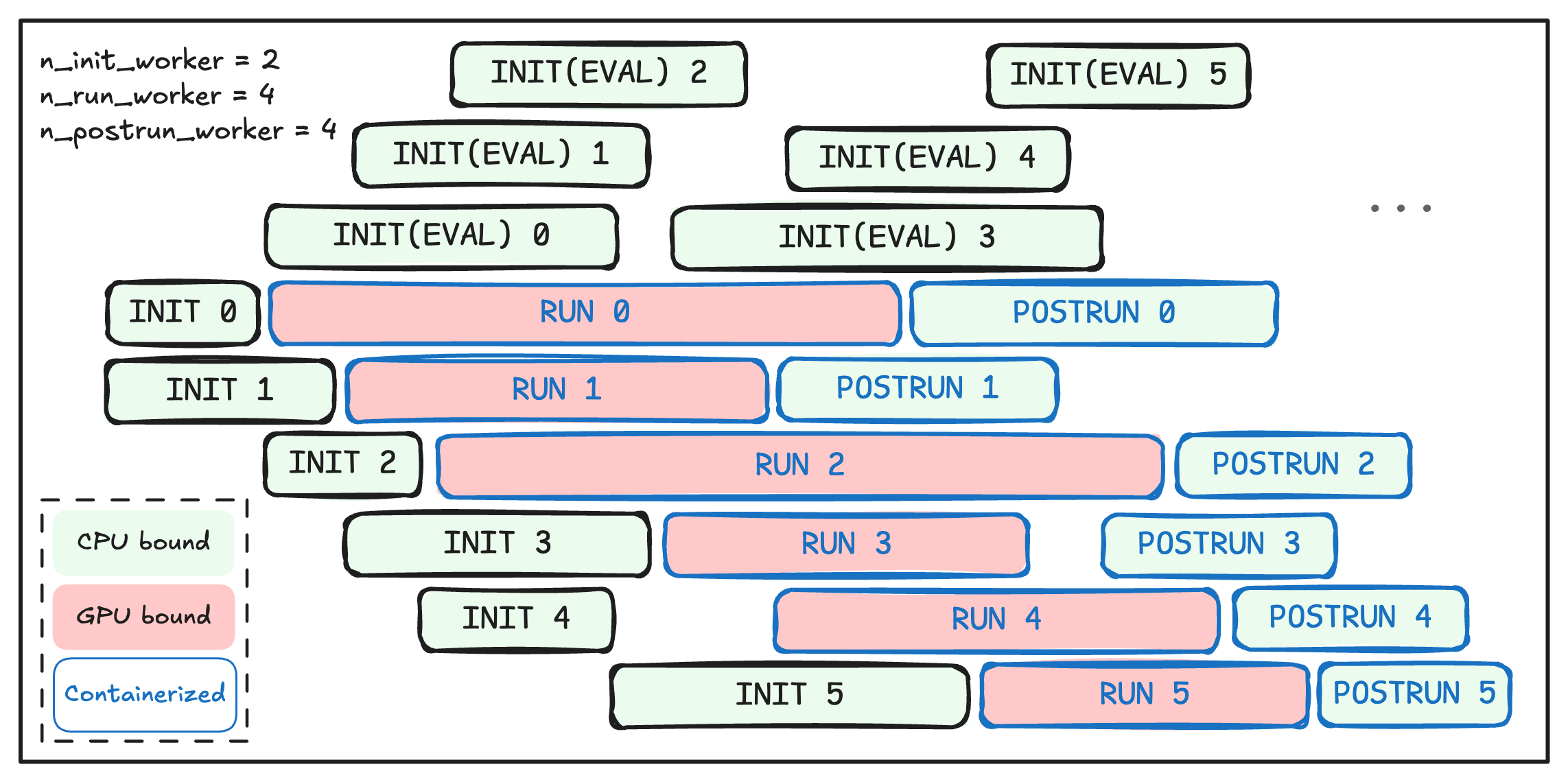
Inside the gateway, INIT prepares runtimes, READY holds a bounded inventory, RUNNING executes harnesses, and POSTRUN reconstructs traces, evaluates results, invokes callbacks and releases resources. The paper also starts clean evaluator-runtime preparation while the harness is running. A slow evaluator should consume a post-run resource rather than occupy a scarce active-run slot.

4.1 A simple capacity model

The following is my explanatory queueing model. Let mean stage times be $t_I,t_R,t_P$, with $c_I,c_R,c_P$ workers. Ignoring shared-resource contention, a necessary capacity bound is

$$\lambda < \min\left\{\frac{c_I}{t_I},\frac{c_R}{t_R}, \frac{c_P}{t_P}\right\}. \tag{4}$$

A serial worker spends $t_I+t_R+t_P$ on a session. Ideal overlap can approach the bottleneck rate rather than that serial rate, but the bound is not a prediction of achieved throughput. Runtime image pulls may contend for storage; evaluators and harnesses may share CPU cores; inference requests share GPU capacity. Long-tail task durations also make mean-based sizing incomplete.

The bounded READY buffer is important because an initialized runtime consumes memory and possibly storage even while idle. Little’s law gives an explanatory relationship $L=\lambda W$ between average in-flight work and its residence time. A buffer large enough to hide preparation delays can improve utilization, but an oversized one accumulates expensive idle environments. Backpressure must eventually reach task admission when post-run evaluation is the bottleneck.

4.2 Algorithm 1: a session lifecycle

The numbered pseudocode below reorganizes Sections 3.1–3.3 and Appendix A.5 for explanation. It is not a claim that the paper provides this exact algorithm or a complete failure-recovery protocol.

Algorithm 1. Staged rollout session
01 Accept a task; create independent session identifiers.
02 Attach runtime, harness, builder, evaluator and deadline.
03 INIT: create the runtime and prepare the harness.
04 READY: wait in the bounded buffer for an execution slot.
05 RUNNING: launch the harness through the gateway proxy.
06 Record each completion with session and policy metadata.
07 Prewarm a clean evaluator runtime when requested.
08 On completion or timeout, stop active harness execution.
09 POSTRUN: reconstruct traces from captured completions.
10 Evaluate artifacts, retaining terminal outcome and status.
11 Return results through the task/callback service boundary.
12 Tear down runtimes and finish session bookkeeping.

The shared deadline keeps an attempt from independently spending a full budget at every stage. Recovering captured calls after a harness timeout is valuable, but a partial trace needs an explicit terminal status. A timeout is not necessarily a failed solution: a correct patch might exist before tests finish. Treating infrastructure failures, budget exhaustion and verified task failure as one reward label can teach the model an accidental property of the execution system.

The paper describes durable results and best-effort cleanup after persistence. It does not establish exactly-once delivery, transactional callback deduplication, or behavior under gateway failure halfway through a call. Those are natural deployment questions, rather than properties I assume from the asynchronous API.

5. Reconstructing trajectories without replacing sampled tokens

5.1 Per-request traces and compatible chains

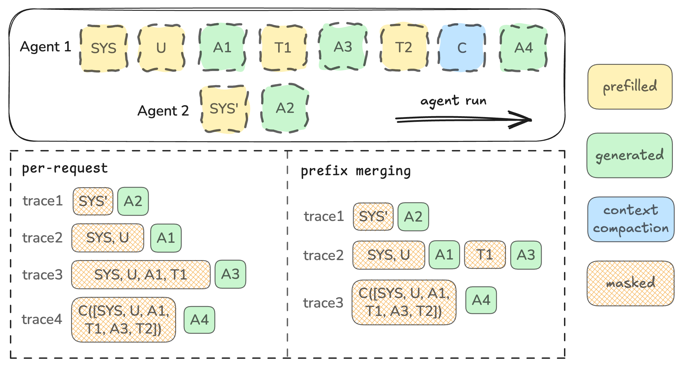
The conservative builder emits one trace per completion. This preserves the context of each individual model call, but can create hundreds of trainer-facing samples for a single task. Prefix merging tries to reduce that fragmentation. It first groups completions using normalized message information and then checks whether the next prompt has the preceding prompt as a strict token prefix:

$$p_{m+1}[1:|p_m|]=p_m. \tag{5}$$

Here indexing follows the paper’s mathematical convention. This condition concerns the old prompt, not the concatenation of the old prompt and sampled response. Compaction, rewritten prompts, and independent subagent histories can therefore split one session into several chains. A session is not assumed to be one append-only conversation.

5.2 Separating the canonical tail from the raw action

For two adjacent calls in a chain, remove the old prompt prefix from the next prompt:

$$t_m=p_{m+1}[|p_m|+1:]. \tag{6}$$

This tail includes a canonical rendering of the previous assistant turn and whatever the harness inserted afterward. Copying the whole tail would replace the sampled response with its retokenized rendering. Polar instead keeps $a_m$ and extracts only the interstitial suffix $u_m$.

Let $e$ be the end-of-turn ID and let $k_m$ be its first position in $t_m$. The rule described in Section 3.4.2 can be written as

$$u_m=\begin{cases} t_m[k_m+1:] & \text{if }a_m\text{ ends with }e,\\ t_m[k_m:] & \text{otherwise}. \end{cases} \tag{7}$$

The distinction prevents duplicating a sampled terminator while still closing the assistant turn when the sampled response does not contain it. This relies on the intended end marker being identifiable. The paper does not give a detailed policy for malformed tails or ambiguous control-token placement. A conservative interpretation is to reject an unsafe merge rather than invent a missing boundary; that is my suggested rule, not a reported implementation result.

5.3 The merged sequence and its mask

For a chain with $K$ completions, the reconstruction is

$$z=p_1\Vert a_1\Vert u_1\Vert a_2\Vert u_2\Vert\cdots\Vert a_K. \tag{8}$$

The first prompt is stored separately. The rest forms the response suffix, even though that suffix includes environment material. The response mask and log-probability arrays must align with every suffix position:

$$\begin{aligned} M&=\mathbf{1}_{|a_1|}\Vert\mathbf{0}_{|u_1|}\Vert \cdots\Vert\mathbf{1}_{|a_K|},\\ L&=\ell_1\Vert\widetilde\ell_{u_1}\Vert\cdots\Vert\ell_K,\\ |M|&=|L|=|z|-|p_1|. \end{aligned} \tag{9}$$

The interstitial log probabilities are synthetic placeholders. Their numerical value should not affect the loss because $M=0$ there. Correctness therefore depends on the trainer honoring the mask before reductions and any ratio-based operations that might otherwise propagate invalid values. The paper’s representative trace in Appendix A.4 illustrates the fields, not a complete test fixture with all lengths expanded.

5.4 Algorithm 2: prefix merging

This pseudocode follows the paper’s construction, with an explicit conservative failure branch that I recommend for underspecified boundaries.

Algorithm 2. Reconstruct token-faithful chains
01 Visit captured completions in recorded order.
02 Find candidate chains using normalized message metadata.
03 Require the previous prompt to be an exact token prefix.
04 If no compatible chain exists, open a new chain.
05 Otherwise append the completion to the chosen chain.
06 For each chain, store its first prompt as prompt_ids.
07 Append each raw sampled response to response_ids.
08 Append its captured log probabilities and an all-one mask.
09 Between calls, isolate the canonical tail's end marker.
10 Extract the interstitial according to Equation (7).
11 Append that context, placeholder logprobs, and zero mask.
12 If the boundary is unsafe, keep the calls separate instead.
13 Emit one trace per chain, retaining session provenance.
14 Assign rewards through the evaluator/trainer contract.

The grouping rule’s tie-breaking is not fully specified in the prose. Identical prompts can occur in repeated or parallel calls. A unique session identity alone does not prove which completion is the causal predecessor of which request. Explicit parent-call metadata would make this relationship stronger than an inference from common prefixes.

5.5 A hand-worked token example

Consider an illustrative one-token prompt $p_1=[10]$, raw response $a_1=[20]$, and next prompt $p_2=[10,21,22,99,30]$. Let $99$ be the turn terminator and suppose decoding token $20$ produces the same text as decoding $[21,22]$. The canonical tail is $[21,22,99,30]$. Since $a_1$ lacks the terminator, $u_1=[99,30]$. If $a_2=[40,99]$, then

$$z=[10,20,99,30,40,99],\qquad M=[1,0,0,1,1]. \tag{10}$$

The five mask entries correspond to the five response positions, excluding the initial prompt. Token $20$ remains trainable, $21$ and $22$ are not substituted, and the inserted terminator and tool token are masked. The final terminator is trainable because it was sampled as part of $a_2$. Trainability follows provenance, not the token’s semantic category.

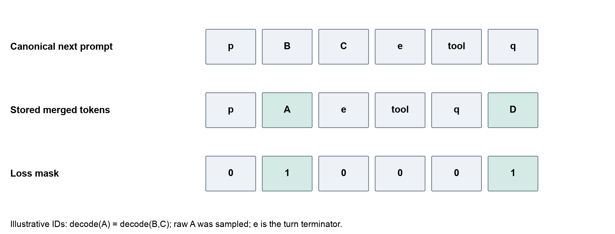
This example also exposes an important limit. The second call originally conditioned on $[10,21,22,99,30]$, while the merged sequence conditions its later response on $[10,20,99,30]$. Equal decoded text does not imply equal model hidden states. Preserving raw actions is necessary, but a stronger exact-context guarantee needs equality of the entire earlier conditioning sequence, or a deliberate mechanism that supplies the original context to each loss segment.

6. Reward assignment is part of the systems interface

Polar can evaluate a final patch in a clean runtime, which reduces the risk that mutated dependencies or test files inside the agent’s working runtime contaminate the score. A built-in evaluator may broadcast the outcome to traces; custom evaluators can supply process or trace-level rewards. This is a useful extensibility point, but the reward contract extends into the trainer.

For an explanatory group-relative estimator, let $G$ sessions attempt the same task, with rewards $R_s$. A common standardized advantage is

$$\bar R=\frac1G\sum_{s=1}^{G}R_s,\qquad A_s=\frac{R_s-\bar R}{\sqrt{G^{-1}\sum_s(R_s-\bar R)^2}+\epsilon}. \tag{11}$$

This equation gives background intuition for GRPO; the paper does not fully specify all trainer reductions. If a session emits $J_s$ traces, averaging equally over traces can weight sessions differently from averaging first within each session. With $g_{s,j}$ representing one trace’s contribution, compare

$$g_{\rm trace}=\frac{\sum_s\sum_{j=1}^{J_s}g_{s,j}}{\sum_sJ_s}, \qquad g_{\rm session}=\frac1G\sum_s\frac1{J_s}\sum_{j=1}^{J_s}g_{s,j}. \tag{12}$$

These estimators generally differ. Neither expression is universally correct: the intended action-level objective, token normalization, and sampling distribution determine the right weighting. The problem is allowing reconstruction to change those choices accidentally. A verbose failed session with 100 request-level traces should not silently become 100 independent reward-group members while a concise successful session contributes one.

Polar reports significant reward hacking when broadcasting outcomes to per-request traces without suitable session normalization or a process reward model. That observation is valuable, but does not prove that terminal rewards themselves are unsuitable for multi-turn agents. It instead motivates documenting the precise interaction between sample expansion, group advantages, token reductions and trace weights. Prefix merging reduces fragmentation; it does not completely solve causal credit assignment or guarantee a fixed number of traces per session.

7. What the online experiments establish

7.1 Training setup and evaluation units

The online study uses Qwen/Qwen3.5-4B, the 293-task training split of NovaSky-AI/SkyRL-v0-293-data, Slime asynchronous GRPO, one epoch, rollout batch size four, and 16 samples per prompt. Appendix A.2 specifies Adam, learning rate $10^{-6}$, weight decay 0.1, and TIS enabled. All four harness experiments use prefix merging and a clean-runtime SWE evaluator. The table explicitly omits cluster topology and worker placement.

The representative payload in Appendix A.3 instead contains eight samples and a 1,200-second timeout. It is an API illustration, not evidence that the online experiments used those exact values. Keeping the hyperparameter table and the example payload distinct avoids manufacturing a contradiction where they describe different purposes.

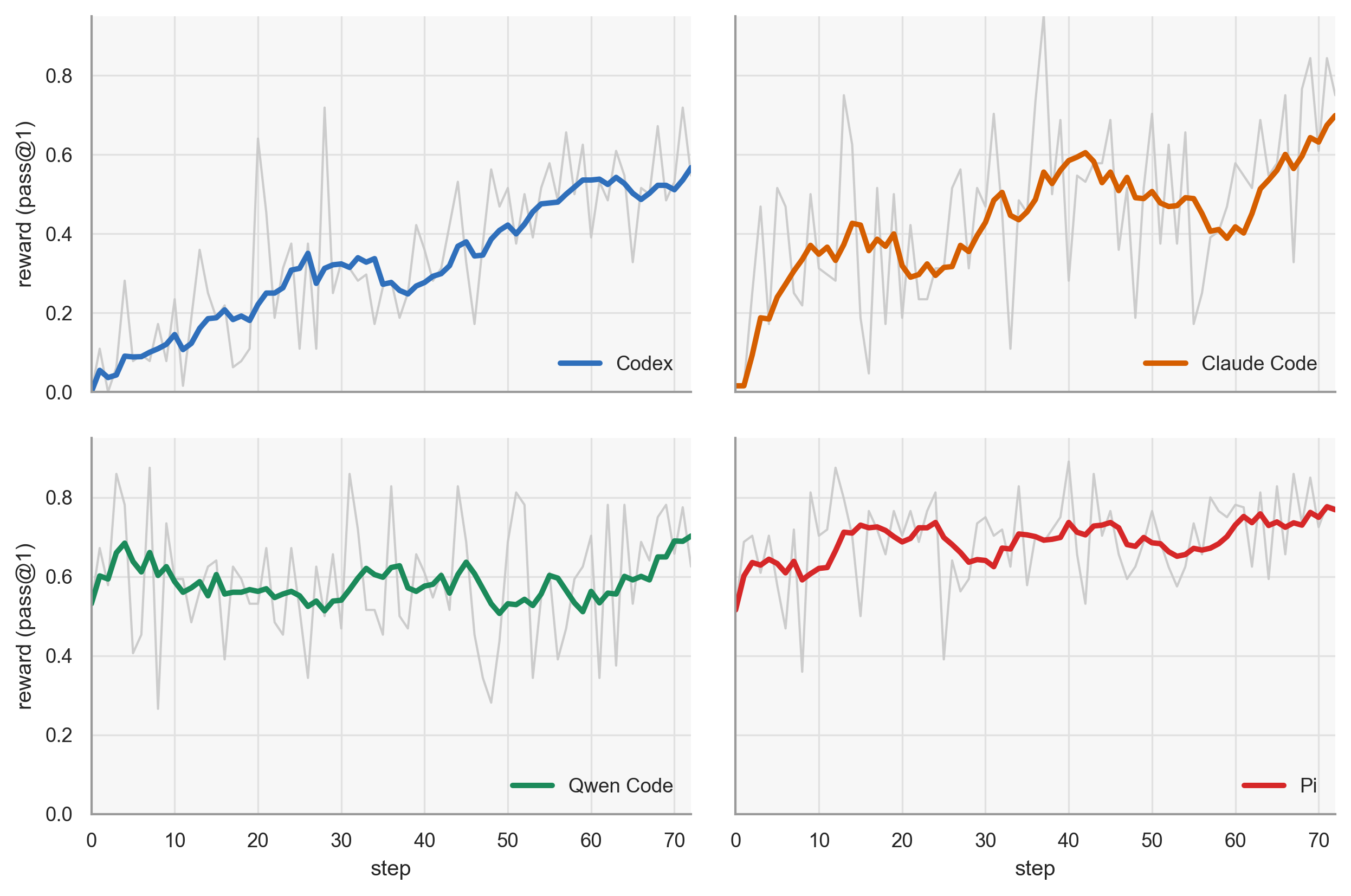
The first-versus-last ten-step averages rise from 9.5% to 54.5% for Codex, 28.8% to 67.0% for Claude Code, 61.6% to 66.0% for Qwen Code, and 61.6% to 76.2% for Pi. These are training-window summaries. They show that optimization can operate through the native interfaces; they are not four estimates of generalization gain.

7.2 Held-out results

Table 1 evaluates pass@1 on SWE-Bench Verified using each corresponding harness. The reported values are:

Harness	Base	Polar RL	Absolute gain
Codex	3.8%	26.4%	22.6 points
Claude Code	29.8%	34.6%	4.8 points
Qwen Code	34.6%	35.2%	0.6 points
Pi	34.2%	40.4%	6.2 points

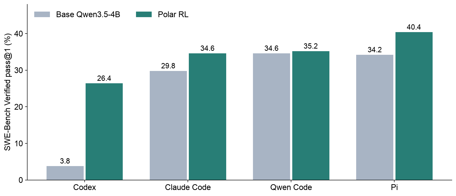
The large Codex improvement is compatible with learning an unfamiliar tool protocol and execution style. The paper offers that explanation, but does not isolate it causally. Harnesses differ in prompts, tools and context policy. A cross-harness matrix, evaluating every trained checkpoint under every harness, would help distinguish protocol adaptation from transferable problem-solving improvements.

The 0.6-point Qwen Code gain is small relative to the claims one might want to make about stable improvement. The paper does not report repeated training seeds or paired task-level uncertainty in this table. I therefore treat the four positive differences as reported observations, without claiming that every difference is statistically established. A low base score can also make a relative improvement look dramatic; the absolute percentage-point values are the appropriate first comparison here.

7.3 Reading the reconstruction speed comparison

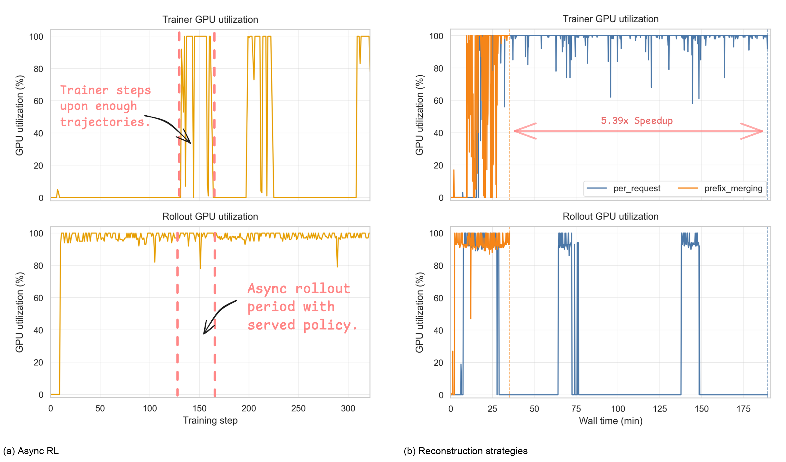
Over the reported three-step window, the per-request strategy emits 1,185 request-level updates and takes 189.5 minutes; prefix merging emits 218 merged-trace updates and takes 35.2 minutes. Average rollout GPU utilization is 20.4% versus 87.7%. Figure 5 in the paper shows the accompanying utilization profiles.

A useful arithmetic check separates sample-count reduction from time reduction:

$$\begin{aligned} \frac{189.5}{35.2}&\approx5.384, & \frac{1185}{218}&\approx5.436,\\ \frac{189.5\times60}{1185}&\approx9.59\ { m s}, & \frac{35.2\times60}{218}&\approx9.69\ { m s}. \end{aligned} \tag{13}$$

These are my calculations from the printed aggregates. The paper reports 5.39 times, a small rounding difference from the rounded times. The nearly matching reductions suggest that fewer trainer-facing units are an important part of the measured effect. They do not establish a faster kernel or equal optimization work. Dividing aggregate time by unit count is only diagnostic accounting, because generation and training overlap; it is not a measured latency per individual trace.

The benefit can still be real. Avoiding repeated prefixes and excessive fragmentation may be exactly the systems improvement required to use heavy harnesses. But a fair efficiency claim should specify whether the invariant is sessions, sampled assistant tokens, training tokens including context, optimizer updates, or held-out quality. Time to a target pass@1 across several seeds would connect the systems result to the learning objective more directly.

8. Offline data generation and an arithmetic inconsistency

The second workload uses a single eight-H100 SGLang job, Qwen3.5-122B-A10B with tensor parallelism eight and maximum model length 32,768, and pi-coding-agent v0.67.68. Sessions run in Apptainer images with Node.js 22. The reported concurrency is five to eight, per-task timeout 3,600 seconds, with one retry for empty generations. These settings belong to the offline case study, not the 4B online training experiment.

The verifier accepts a patch only when all FAIL_TO_PASS tests become successful and all PASS_TO_PASS tests remain successful. The paper reports 504 accepted trajectories from 1,638 attempts, 30.8% acceptance, at approximately 64 GPU-hours. Accepted sessions average 104 messages and 51 assistant turns, with a long tail beyond 200 turns. The released data has a repository-stratified 90/10 split.

I found two discrepancies within Table 2 itself:

$$\begin{aligned} 343+257+71+81+219+477+141&=1589\ne1638,\\ 184+101+27+24+45+98+25&=504,\\ 100\times98/477&\approx20.5\ne19.7. \end{aligned} \tag{14}$$

The seven accepted counts sum correctly, but their attempt counts are 49 below the printed total. The pandas rate printed as 19.7% does not follow from 98 accepted out of 477 attempts. The PDF and HTML both show these entries. I retain the paper’s numbers rather than guessing whether retries, omitted attempts, or a typographical error explains them.

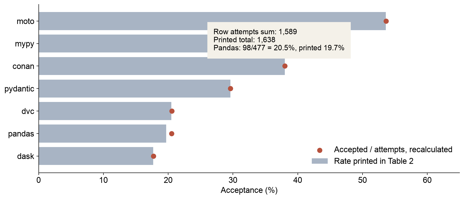
The aggregate 504/1,638 does round to 30.8%; using the sum of row attempts gives approximately 31.7%. Until the denominator is clarified, both calculations should remain attached to their definitions. Likewise, 64 GPU-hours divided by 504 is about 7.62 GPU-minutes per accepted trajectory under the reported aggregate accounting. That is a coarse resource ratio, not a marginal price, a wall-clock session latency, or a cost figure with CPU and runtime preparation included.

A repository-stratified split ensures repository representation; it does not establish independence between closely related issues, overlapping files, or patches with common ancestry. Also, filtering successful patches conditions the corpus on verifier acceptance. Long unproductive exploration can remain inside a successful trajectory, and verifier success is narrower than general patch correctness. The paper demonstrates an effective data-production pipeline without proving that downstream SFT quality is optimal.

9. Design choices, alternatives, and failure boundaries

Several choices make sense together, but each buys something specific. I would compare them through the following questions rather than rank every system with a single feature score.

Choice	Reason to choose it	Alternative and boundary
Model API proxy	Works across native executable boundaries	In-process tracing exposes richer state but requires instrumentation
Per-request traces	Keeps each call’s original prompt	Prefix merging reduces fragments but needs compatible histories
Separate post-run workers	Prevents evaluation from occupying run slots	A single pool is simpler but mixes blocking costs
Fresh evaluator runtime	Scores the patch away from agent mutations	Reusing the agent runtime is cheaper but may contaminate tests
Terminal patch reward	Directly measures the benchmark outcome	Process rewards add resolution but introduce judge error

The feature matrix in Appendix A.1 is the authors’ characterization of contemporary systems, not an independently established speed or quality ranking. The appendix itself acknowledges partial support and explains why model gateways, generic observability and full runtime lifecycle services are not identical abstractions. I use that matrix to understand the intended contract, rather than treat every cross as proof that a neighboring framework cannot support a workload.

A particularly important design axis is who owns policy freshness. Polar records policy-version metadata and serves asynchronous trajectories, while a trainer decides how to consume them. The existence of that field does not guarantee that every token in a long session was generated under one immutable checkpoint. If serving weights change between calls, a session can contain several behavior versions. Per-token log probabilities help only if they remain matched to those actions and the trainer uses a suitable estimator.

Another axis is feedback latency. Fast sessions reach the learner sooner, while difficult sessions linger in runtime or evaluation queues. If the trainer updates from whichever groups arrive first, the early training stream can favor easy problems. Explicit timeout and retry rules can further alter the distribution. These are consequences of asynchronous sampling, not reasons to reject it, but they should be measured alongside utilization.

10. Limitations of the paper and this reading

The empirical scope is concentrated on coding harnesses, a 4B base model for online RL, and one larger teacher for offline generation. API support for a multimodal provider is not the same as a demonstrated computer-use or vision-action training result. Broad harness portability is an architectural goal with several concrete examples, not an exhaustive universality test.

The online efficiency study lacks the topology and worker-placement details needed to interpret absolute capacity. A three-step utilization window gives useful mechanism evidence but not a sustained scaling result across cluster sizes. Error bars, repeated seeds, and a fully specified relation between traces and optimizer updates would strengthen the quantitative claims. The offline denominator inconsistency also limits precise cost and acceptance comparisons.

My formulas for queue capacity, policy gradients, estimator weighting and uncertainty requirements are explanatory analysis. They are not additional theorems or measurements reported by the authors. I have read the 17-page paper, including Appendix A.1–A.5, checked its figures and printed arithmetic, and have not run training or generated new benchmark results. The figures labelled as redraws retain reported data; the token example is synthetic and hand-worked.

11. Critical analysis: what I would change next

11.1 Specify context fidelity separately from action fidelity

Polar’s most interesting unresolved issue is the interaction of retokenization drift with merged conditioning histories. For a later action, write its original prefix as $h^{\rm old}$ and its reconstructed prefix as $h^{\rm new}$. Exact importance-ratio interpretation requires

$$h^{\rm new}=h^{\rm old},\qquad \rho=\frac{\pi_\theta(a\mid h^{\rm old})} {\pi_b(a\mid h^{\rm old})}. \tag{15}$$

If the numerator instead uses $h^{\rm new}$, it compares different conditional events. Even when the token ID $a$ is correct, a mask cannot make those contexts equal. Replacing a canonical assistant span with raw sampled IDs may change sequence length, positions, and the representations available to later tokens. Matching decoded strings does not supply a theorem of conditional-distribution equivalence.

I would document an exactness mode that merges only when reconstructed prefixes equal the original call prefixes. Where that condition fails, retaining separate calls is the safe baseline. A more ambitious alternative is segmented training that preserves each call’s original context while sharing compatible prefix computation. That approach should be evaluated as a distinct training representation, because it may sacrifice some of the simplicity or savings of one flattened trace.

This is a conditional critique of the construction as described. It is not a claim that every Polar trajectory has this mismatch or that the reported gains disappear. If canonical and raw histories coincide in the studied workloads, the counterexample does not apply there. Reporting the mismatch frequency and its effect on recomputed log probabilities would resolve the scope of the concern.

11.2 Hold the learning unit constant in efficiency claims

The next experiment I would want is a matched accounting study. Keep the sampled sessions fixed, report generated action tokens, total processed tokens, trace counts, actual optimizer updates, and stage-level wall time. Then compare time and GPU-hours to the same held-out quality. Prefix merging should be allowed to win through less redundant context processing; it should not receive credit merely because a different sample reduction silently changes the optimization budget.

The paper’s request-versus-merged comparison is a useful starting point precisely because the unit-count ratio nearly matches the runtime ratio. That makes the mechanism inspectable. A short analysis of loss normalization and reward grouping would turn it into much stronger evidence about learning efficiency.

11.3 Make the asynchronous boundary statistically visible

I would report policy age in optimizer steps, session duration, number of calls, and number of reconstructed chains, jointly with reward. Long sessions can have older policies and lower success rates, so aggressive stale-data rejection can bias the task distribution. Similarly, a clean evaluator should return infrastructure failure separately from verified patch failure. A report of how many samples are dropped, retried or truncated would show whether utilization gains change which tasks train the model.

For offline generation, release the attempt ledger needed to reconcile Table 2, including how retries enter the denominator. Evaluate the resulting SFT model rather than only the accepted trajectory count, and use issue- or patch-aware deduplication in addition to repository stratification. These changes answer specific uncertainty in the paper without requiring a new central architecture.

12. Reproducibility notes and conclusion

The minimum conceptual record for interpreting a run includes the task and session IDs, harness configuration, model identity, call-level behavior information, original prompts, sampled IDs, masks, evaluator outcome and terminal status. The online hyperparameters in Appendix A.2 should be distinguished from the illustrative payload in A.3 and from the offline configuration in Section 4.2. The missing cluster topology and unspecified reductions remain questions to resolve before comparing resource efficiency precisely.

My practical conclusion is that Polar identifies an effective systems abstraction: train the model inside the harness that will actually use it, and collect the training contract at the model boundary. Its stage separation and raw-token capture solve concrete sources of integration friction. The strongest next step is to state more precisely when reconstruction preserves the original conditional events and when reduced fragmentation preserves the intended optimization weighting. Those conditions would make the portability and utilization story easier to trust and extend.

References and resource pointers

• Xu et al., Polar: Agentic RL on Any Harness at Scale, v1. Primary source for methods, Figures 1–6, Tables 1–4, and Appendix A.1–A.5.
• Official project resource linked in the paper.
• SWE-Gym training data identified in the paper.
• Offline trajectories identified in the paper.