VHA: Train with Virtual Heads, Deploy as Ordinary GQA

Review date: 2026-11-04 · Author: Zhongzhu Zhou
Paper: Virtual Head Attention
Paper authors: Xibo Ding, Guoxia Wang, Jinle Zeng, Jiabin Yang, Sirui Tao, Chao Yang, Dianhai Yu
arXiv: 2610.17959 · Version: v1, 2026-10-13

1. A different training graph can produce an ordinary inference graph

Reducing the number of key/value heads is an unusually practical way to shrink a language model’s cache. It preserves ordinary dense attention and uses familiar grouped-query attention kernels. The difficulty is quality: many query heads must retrieve information from the same small collection of keys and values. Simply reducing the query-head count as well may save projection work, but removes independent attention distributions.

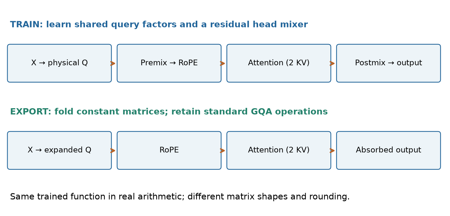
Virtual Head Attention, or VHA, takes a more indirect route. During training, it computes half as many physical query heads, transforms each of them separately for two KV groups, and thereby recovers the original number of attention heads. A second linear module mixes the resulting head outputs through a low-rank residual. After training, the two modules can be multiplied into the query and output projection matrices. The deployed model then has a standard GQA structure with two KV heads. [1, Sections 3–4]

The interesting claim is therefore about parameterization and optimization. It is not that a new nonlinear inference operator is indispensable for good attention. Nor does the paper give a lossless conversion of an arbitrary existing eight-KV-head checkpoint into a two-head checkpoint. Its models are trained with the VHA parameterization. Exact folding preserves the function of that trained VHA model in real arithmetic; the architectural choice to share KV heads is a separate issue.

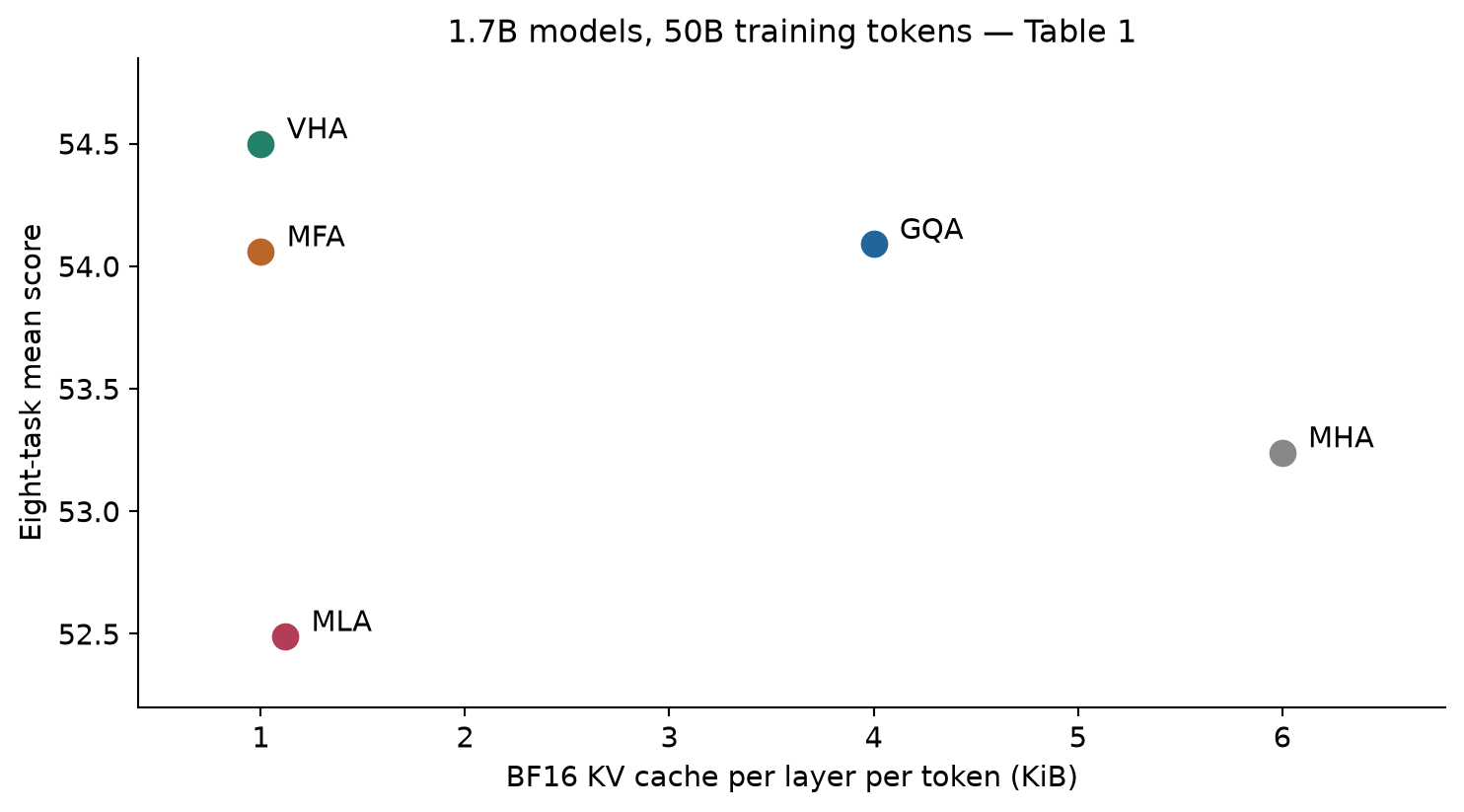
At 1.7B scale, the reported eight-task mean rises from 54.09 for GQA to 54.50 for VHA, while BF16 KV storage falls from 4 KiB to 1 KiB per layer per token. The corresponding arithmetic estimate falls from 10.61 to 9.78 GFLOPs per token for training. A separate long-context experiment shows substantially larger retrieval gains. These are promising results, but they are three different kinds of evidence: downstream scores, a storage identity, and an analytical operation count. The paper does not report an end-to-end decoding throughput benchmark that turns its theoretical speedup discussion into a measured latency claim.

I read the complete 21-page paper, including Appendices A–H. This review reconstructs its equations with an explicit head ordering, checks the tables against the narrative, and separates reported results from calculations made here. That distinction matters particularly for the relation between the factored training graph and the expanded query projection used by the simplest folded serving graph.

2. Prerequisites: what is shared, what is cached, and what stays quadratic

2.1 Three head counts, rather than one

Let the input be $X\in\mathbb R^{S\times h}$, where $S$ is sequence length and $h$ is model width. Each head has width $d$. I use $G$ for the number of KV groups, $m$ for the number of physical query heads, and $H_v=Gm$ for the number of virtual query heads. This notation deliberately distinguishes a KV-group count from the number of query heads sharing one KV head.

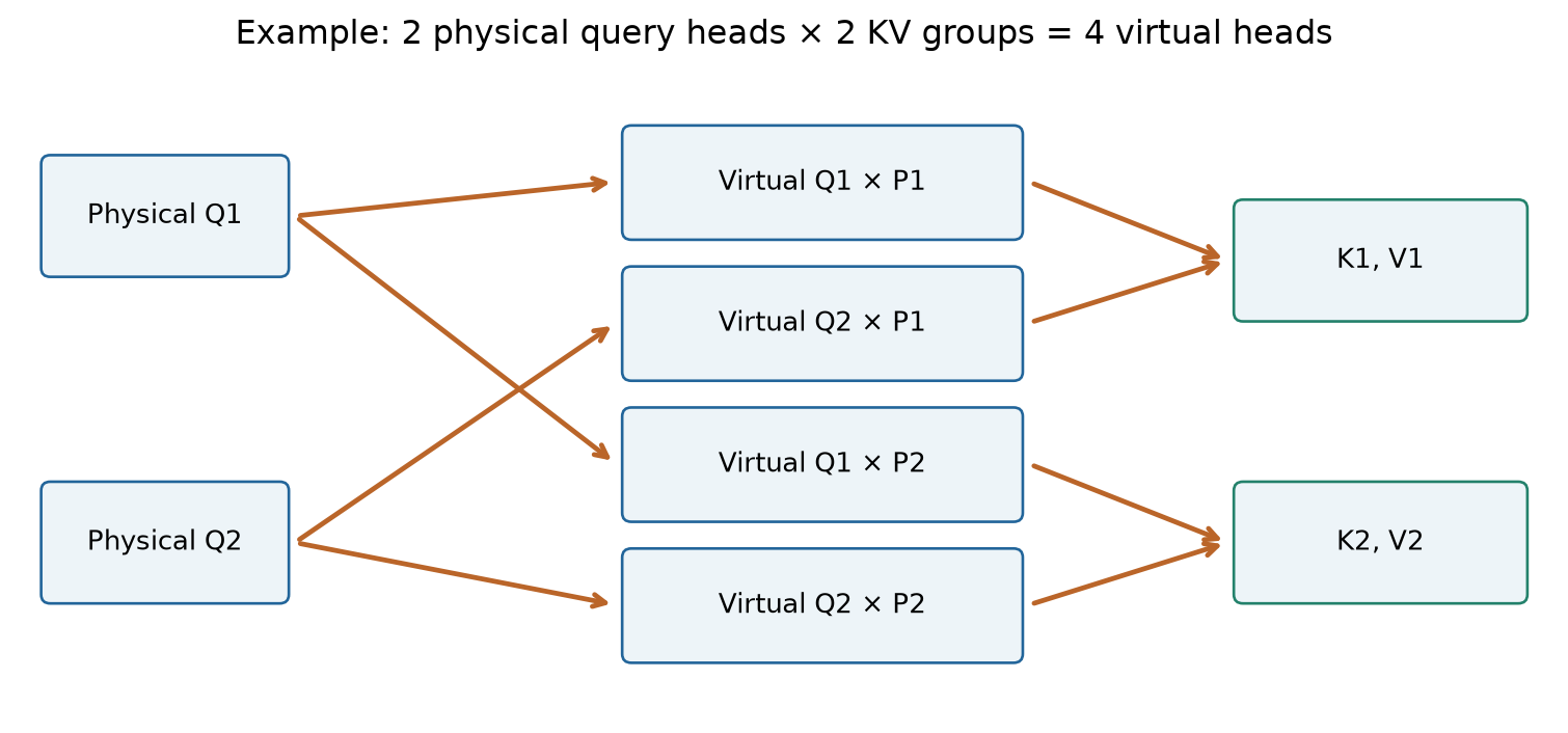
The paper sets $G=2$ and $m=H_q/2$, where $H_q$ is the original query-head count. Thus $H_v=H_q$. In the 1.7B configuration, eight physical query heads become sixteen virtual heads, which attend to two KV heads. The phrase “halve the query heads” refers to the first projection, not to the number of final attention distributions. This is why comparing VHA with an ordinary eight-query-head GQA model needs care.

In conventional GQA, query heads assigned to a group use the same $K_g,V_g$ but still have their own queries. For head $(i,g)$, suppressing positional encoding temporarily, attention is

$$Y_{i,g}=\operatorname{softmax}\!\left( \frac{Q_{i,g}K_g^\top}{\sqrt d}+C \right)V_g, \qquad Y_{i,g}\in\mathbb R^{S\times d}. \tag{1}$$

Here $C$ is the causal mask, with forbidden positions assigned negative infinity. Sharing keys and values does not force identical attention weights, because the queries differ. But it restricts the representations against which those queries are compared and the value vectors they retrieve. VHA tries to make this stronger sharing easier to train, while preserving the original number of query-dependent distributions.

2.2 The cache equation is simple, but its scope matters

For ordinary BF16 keys and values, one token contributes two tensors, each containing $Gd$ numbers at two bytes per number. With batch size $B$, $L$ full-attention layers and $S$ cached positions,

$$M_{\mathrm{KV}}=2\times2\times BLSGd =4BLSGd\quad\text{bytes}. \tag{2}$$

At $d=128$, eight KV heads require 4,096 bytes per layer per token; two require 1,024 bytes. I label these values 4 KiB and 1 KiB, although the paper uses “KB.” For a hypothetical batch-one, 28-layer, 131,072-token cache, this is 14 GiB versus 3.5 GiB. That calculation excludes weights, activations, allocator overhead, temporary workspaces and any non-attention state. It is an illustration of Equation 2, not a reported capacity test.

Queries are transient in standard autoregressive decoding; old queries do not need to be retained in the KV cache. Expanding query heads therefore does not directly cancel the KV-memory reduction. It can still affect projection work, temporary activations and attention arithmetic. “Cache-free extra heads” would be misleading if interpreted as “computation-free extra heads.”

2.3 Dense attention has not become sparse or linear

VHA retains $H_v$ attention distributions over all causally visible positions. The query–key and probability–value products still have dense-attention scaling. Reducing the first query projection’s width does not halve those products, because the virtual expansion restores the query-head count before attention. Long sequences can therefore make the quadratic attention term dominate a smaller projection saving.

This is also different from selecting top-$k$ tokens, evicting old cache entries, or storing quantized keys. The basic model retains every position’s two KV heads. Such techniques might later be combined with VHA, but their approximation errors and latency effects are not evidence supplied by this paper. Keeping the mechanism separate helps explain why VHA can use an ordinary GQA serving path after folding.

2.4 RoPE fixes the order of the linear operations

The architecture diagram places Premix before rotary position embedding. For row vectors at position $t$, write the rotary transform as $R_t$. The relevant query is $(x_tW_iP_g)R_t$. A constant matrix can be absorbed into the projection before this positional transform. It cannot generally be moved through the position-dependent rotation, because $P_gR_t$ need not equal $R_tP_g$.

This ordering is easy to lose when writing a compact attention equation. I retain it in the algorithms below. The paper’s algebraic absorption argument is valid because the constant transforms remain on the appropriate side of RoPE; no commutation assumption is needed. An alternative placement after RoPE would require a different derivation and would not automatically inherit the same simple export rule.

3. Premix: a shared query basis with group-specific transformations

3.1 Expand features, not a list of independent learned heads

Split the physical query projection into $m$ matrices $W_i\in\mathbb R^{h\times d}$. Let each KV group have a learned matrix $P_g\in\mathbb R^{d\times d}$. The computation is

$$Q_i=XW_i,\qquad \widetilde Q_{i,g}=Q_iP_g=X(W_iP_g), \qquad i=1,\ldots,m,\quad g=1,\ldots,G. \tag{3}$$

Every physical query head is reused in every KV group. Within a group, the same $P_g$ transforms all physical query heads. It acts on the $d$ feature channels; it is not an average over the query-head axis. The pair $(i,g)$ identifies a virtual head. Different $P_g$ matrices let the same physical representation ask different questions of different KV groups.

The construction replaces $Gm$ freely learned query matrices with $m$ shared matrices and $G$ smaller transformations. The effective matrix of virtual head $(i,g)$ is

$$W^{\mathrm{eff}}_{i,g}=W_iP_g. \tag{4}$$

This is a structural sharing constraint. Each individual product can still have rank $d$, so calling every virtual query projection “low rank” is not generally correct. The important restriction is that different effective projections share factors. Postmix, discussed next, contains the explicitly low-rank residual.

3.2 Why the initialization starts close to duplicated heads

The paper initializes $P_g=I+\alpha\epsilon_g$, using a small Gaussian perturbation and default $\alpha=0.1$. Initially, the two versions of a physical query are related, while the perturbation permits them to diverge. The two groups also have different learned keys and values, so similar queries alone do not imply identical attention outputs.

There is a useful design tension here. Fully independent virtual-head projections provide more freedom but give up the parameter and projection savings. Exactly identical transforms could preserve too much symmetry in the query factors. A lightly perturbed identity is a compromise: preserve the physical query’s meaning while letting group-specific structure emerge. The appendix’s initialization experiment supports this as a useful quality prior, rather than proving that other initializations cannot train.

3.3 Shared factors couple the training signals

Let $D_{i,g}$ be the gradient of the loss with respect to $\widetilde Q_{i,g}$. Matrix differentiation gives

$$\frac{\partial\mathcal L}{\partial W_i} =\sum_g X^\top D_{i,g}P_g^\top, \qquad \frac{\partial\mathcal L}{\partial P_g} =\sum_i (XW_i)^\top D_{i,g}. \tag{5}$$

The first expression adds learning signals from different KV groups into the same physical query matrix. The second pools signals from different physical heads into the same group transform. Consequently, two effective heads do not evolve as independent dense query matrices would. Even when their forward computation can be represented by an ordinary projection, the parameter updates follow a different geometry.

This coupling can serve as useful regularization if the heads benefit from a shared basis. It can also create interference if different groups need incompatible changes. The paper’s results show that the selected parameterization works well in its tested settings; Equation 5 explains why that is an empirical optimization result, not a universal consequence of matrix associativity.

4. Postmix: a low-rank residual that disappears into the output projection

4.1 State the axis and matrix orientation explicitly

For one token, arrange the attention outputs in a matrix $Y\in\mathbb R^{H_v\times d}$, with one head per row. Let $A,B\in\mathbb R^{H_v\times r}$. The paper’s head-axis residual can be written

$$Y'=Y+B(A^\top Y)=MY, \qquad M=I_{H_v}+BA^\top. \tag{6}$$

First, $A^\top$ collects the head outputs into $r$ intermediate mixtures. Then $B$ distributes those mixtures back to the $H_v$ heads. The identity branch preserves the original outputs. The rank bound applies to $M-I$, not to $M$ itself: adding identity usually leaves a full-rank transform. This distinction is important when discussing information loss or invertibility.

The default bottleneck is $r=m/2$. At 1.7B, $m=8$, $H_v=16$ and $r=4$. The two factor matrices contain only $2H_vr=128$ parameters. The operation is shared across token positions and feature channels. It provides a compact, structured way to change how head outputs contribute to the layer, rather than assigning a different arbitrary mixing matrix to every token.

The paper initializes $A$ with small random values and $B$ to zero. Therefore $M=I$ at initialization. The added branch begins as a no-op; gradients can update $B$ immediately, while the gradient to $A$ through that branch initially vanishes because it is multiplied by $B$. Initializing both factors to zero would instead stall both factor gradients in the simple bilinear branch. The asymmetric initialization is a meaningful design choice.

4.2 Derive the output-folding rule without hiding a transpose

Let $\operatorname{rowflat}(Y)$ concatenate the head rows into a row vector. Mixing the head axis produces

$$\operatorname{rowflat}(MY) =\operatorname{rowflat}(Y)(M^\top\otimes I_d). \tag{7}$$

To see the transpose, the new head $j$ is $\sum_i M_{ji}Y_i$. Its contribution to the final output is multiplied by output block $W_{O,j}\in\mathbb R^{d\times h}$. Reordering the sum gives

$$\begin{aligned} \sum_j\left(\sum_i M_{ji}Y_i\right)W_{O,j} &=\sum_iY_i\left(\sum_jM_{ji}W_{O,j}\right),\\ W'_{O,i}&=W_{O,i}+\sum_j(BA^\top)_{ji}W_{O,j}. \end{aligned} \tag{8}$$

Equivalently, for a row-vector implementation,

$$W'_O=\bigl((I+AB^\top)\otimes I_d\bigr)W_O. \tag{9}$$

The apparently reversed factor order in Equation 9 follows from the transpose in Equation 7. Writing the head layout first avoids confusing the head-space matrix with its flattened representation. The factors’ names could be exchanged without changing the idea, but an export procedure must use one convention consistently.

There is no need to materialize the large Kronecker matrix. Define $C_k=\sum_j B_{jk}W_{O,j}$. Then $W'_{O,i}=W_{O,i}+\sum_k A_{ik}C_k$. This blockwise multiplication implements the same algebra at export time and makes the dimensional compatibility explicit. It also shows that folding does not require $M$ to be invertible: multiplication is valid even if training has made the mixer singular.

4.3 Why linearity is retained

A nonlinear activation between the factors would generally prevent replacing the branch with one fixed output matrix. VHA deliberately avoids that complication. This does not make the whole attention layer linear: the softmax attention weights still depend nonlinearly on the input. Only the extra modules are linear and position independent.

The SiLU ablation supports this choice within the tested 1.7B setup. Adding SiLU to Premix, Postmix, or both yields task means of 53.83, 53.79 and 53.67, versus 54.50 for the linear design. These measurements show no quality benefit from those particular nonlinear variants, while the export disadvantage follows algebraically. They do not establish that every nonlinear cross-head architecture is inferior.

5. Algorithms: training form and inference export

5.1 Algorithm 1 — forward computation with explicit virtual heads

The following numbered pseudocode expresses the paper’s mathematical method, not a claim about repository internals. Batch dimensions are omitted. Head order is group-major, then physical-head index, and all tensors using this order must agree.

01 Input: X[S,h], physical query blocks W[i], KV weights, A, B
02 Set G = 2, m = number of physical query heads, Hv = G*m
03 Project K = X*WK and V = X*WV into G heads of width d
04 For each physical head i = 1,...,m:
05     Q[i] = X*W[i]
06 For each KV group g = 1,...,G:
07     Krot[g] = RoPE(K[g], positions)
08     For each physical head i = 1,...,m:
09         j = (g-1)*m + i
10         Qvirtual[j] = Q[i]*P[g]
11         Qrot[j] = RoPE(Qvirtual[j], positions)
12         Scores[j] = Qrot[j]*transpose(Krot[g])/sqrt(d)
13         Prob[j] = softmax(Scores[j] + causal_mask)
14         Y[j] = Prob[j]*V[g]
15 For each token t:
16     U[t] = transpose(A)*Y[t]             # r by d
17     Ymixed[t] = Y[t] + B*U[t]            # Hv by d
18     Output[t] = rowflat(Ymixed[t])*WO
19 Return Output; use ordinary backpropagation for training

The virtual expansion sits before the attention operator. Postmix sits after the probability–value product. Neither changes the causal mask. Thus a current token receives no future information, even though its current head outputs are mixed. Causality follows from the already masked head outputs and positionwise mixing, not from a special new masking rule.

This algorithm is deliberately readable rather than a memory-allocation prescription. A production training kernel may fuse or tile operations to avoid materializing some intermediates. The paper’s mathematical result does not require a particular materialization strategy, and the review does not treat a pseudocode tensor as proof of peak accelerator memory.

5.2 Algorithm 2 — fold a trained checkpoint

Export freezes the learned matrices and replaces compositions of linear maps with their products. The sequence-dependent operations remain in their original positions.

01 Input: trained W[i], P[g], WK, WV, WO, A, B
02 Preserve head order j = (g-1)*m + i
03 For each group g and physical head i:
04     WQ_export[j] = W[i]*P[g]              # h by d
05 Split WO into Hv blocks WO[j], each of shape d by h
06 For each bottleneck coordinate k = 1,...,r:
07     C[k] = sum_j B[j,k]*WO[j]
08 For each virtual head i = 1,...,Hv:
09     WO_export[i] = WO[i] + sum_k A[i,k]*C[k]
10 Concatenate WQ_export blocks in the recorded head order
11 Concatenate WO_export blocks in that same head order
12 Keep WK, WV, RoPE, causal masking and other layers unchanged
13 Configure standard GQA with Hv query heads and G KV heads
14 Remove the explicit Premix and Postmix operations
15 Export the frozen inference parameters

The mathematical contract is equality before and after export over real numbers. Floating-point matrix products have different rounding when multiplication is reassociated. Quantization scales may also change when factors are merged. Therefore “exactly absorbable” should not be read as a guarantee of bitwise-identical BF16 logits or identical sampled text under every implementation. This is a numerical boundary of the algebra, not evidence that the paper reports a failure.

The export also changes the shape of the query projection: it now has $H_v$ heads, not $m$. That expanded representation is precisely what makes the serving graph conventional. A serving system could keep the factors to preserve their projection arithmetic, but then it has chosen a different execution path with explicit extra operations. Both choices are reasonable; they should not be assigned the same cost model automatically.

6. Cost accounting: parameters, FLOPs, bytes and latency

6.1 Query parameters and query arithmetic are different ratios

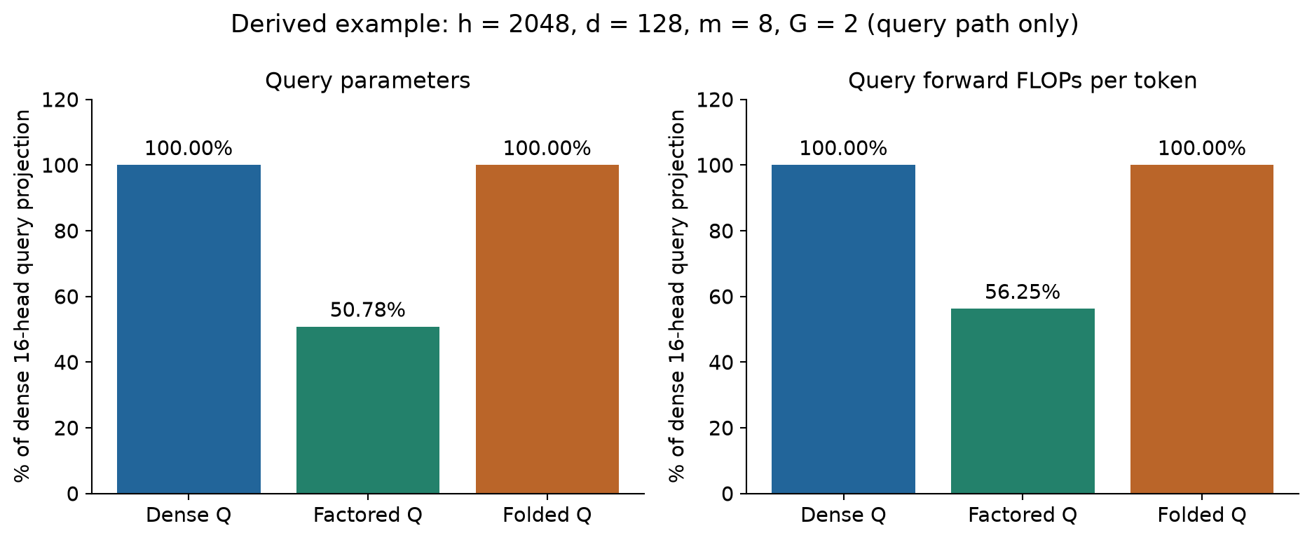
For the dense query projection, the parameter count is $Gmhd$. For the factored representation it is $mhd+Gd^2$. Dividing gives

$$\rho_{\mathrm{param}} =\frac{mhd+Gd^2}{Gmhd} =\frac1G+\frac{d}{mh}. \tag{10}$$

Count one multiply and one add as two FLOPs. The physical query projection costs $2Smhd$. Applying each $P_g$ to all $m$ physical query heads costs $2SGmd^2$. Therefore the corresponding forward-arithmetic ratio is

$$\rho_{\mathrm{Q,FLOPs}} =\frac{2Smhd+2SGmd^2}{2SGmhd} =\frac1G+\frac dh. \tag{11}$$

The difference comes from reuse: each group transform has only $d^2$ parameters, but is applied to $m$ heads. With $h=2048,d=128,m=8,G=2$, the factored query has 2,129,920 parameters versus 4,194,304, or 50.78%. Its forward arithmetic is 4,718,592 FLOPs per token versus 8,388,608, or 56.25%. These calculations describe the query path alone. They do not predict a 43.75% reduction for the complete Transformer.

6.2 Whole-model training estimates are much smaller

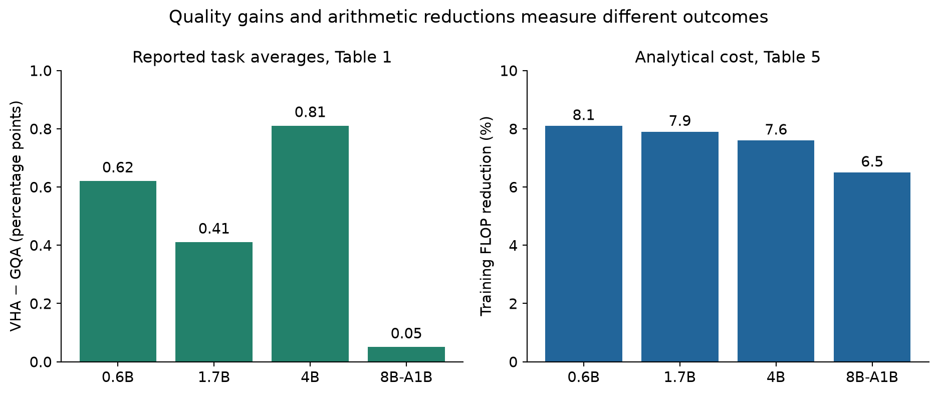
Table 5 includes the other Transformer work and reports training FLOP reductions of 8.1%, 7.9%, 7.6% and 6.5% against the selected GQA baselines at 0.6B, 1.7B, 4B and 8B-A1B. The 1.7B numbers are 10.61 versus 9.78 GFLOPs per token at sequence length 4,096. Recomputing from those rounded values gives about 7.8%; the table’s 7.9% should be understood with its reported precision.

The cost comparison also depends on the baseline architecture. MHA has a larger cache but lower reported training FLOPs than VHA in several rows. Thus the attractive result is a cache–quality–compute trade-off, not a claim that VHA minimizes every resource against every alternative. MFA is especially useful in this comparison: its 1 KiB cache matches VHA’s, but its reported 1.7B training cost is 15.90 GFLOPs per token and its task mean is 54.06.

After full folding, the query-factor savings in Equation 11 are no longer available to an ordinary expanded query GEMM. The two-KV-head design still saves KV-projection work relative to an eight-head baseline. But the factored training/prefill graph and the fully folded inference-prefill graph should be measured separately. The paper’s compatibility argument is strong; its arithmetic accounting should not be casually transplanted across these graph choices.

6.3 Less cache traffic does not imply the same end-to-end speedup

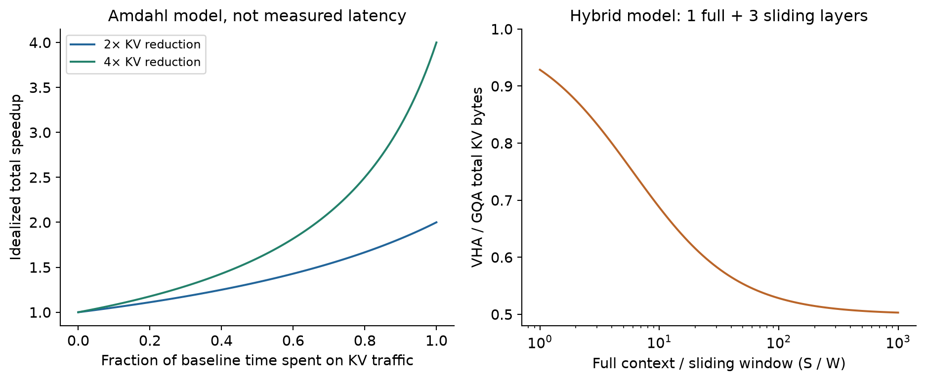
The paper discusses a theoretical two-to-fourfold gain for memory-bound decoding, motivated by fewer KV bytes. Suppose, as a deliberately simplified model, that a fraction $f$ of baseline time is proportional to KV traffic and that this portion shrinks by a factor $c$. The total speedup is

$$\mathrm{speedup}_{\mathrm{ideal}} =\frac{1}{(1-f)+f/c}. \tag{12}$$

For $c=4$, an 80% KV-traffic share gives 2.5×, while a 50% share gives 1.6×. These are analytical examples, not measurements of VHA. Weight reads, feed-forward work, communication, launch overhead and memory-access efficiency can all limit the benefit. A smaller cache can also enable a larger batch; that is a throughput opportunity with its own latency implications, rather than a fixed speed multiplier.

6.4 Hybrid sliding-window models need a different memory denominator

The long-context study changes full-attention KV heads from four to two, but leaves sliding-window layers at eight KV heads. Its full-to-sliding layer ratio is 1:3. If the full context is $S$ and the sliding window is $W$, ignoring common factors, the cache ratio becomes

$$\frac{M_{\mathrm{VHA}}}{M_{\mathrm{GQA}}} =\frac{\tfrac14(2S)+\tfrac34(8W)} {\tfrac14(4S)+\tfrac34(8W)} =\frac{0.5S+6W}{S+6W}. \tag{13}$$

It approaches one half only when full-context storage dominates. At the illustrative ratio $S=W$, it is approximately 0.929. The exact window and allocation policy determine a real model’s total bytes. Reducing the full-attention component by two therefore cannot be advertised as halving all hybrid-model cache memory without specifying the context and window.

7. Experimental evidence: which comparisons answer which questions?

7.1 The main small-scale study tests a practical trade-off

The main Qwen3-family experiments train 0.6B, 1.7B, 4B and 8B-A1B models on 50B FineWeb-Edu tokens, at context length 4,096 with BF16 training. Table 1 averages eight downstream tasks. Its results are summarized below; the deltas are percentage-point differences between reported mean scores.

Scale	GQA mean	VHA mean	VHA − GQA	GQA / VHA KV KiB
0.6B	50.42	51.04	+0.62	4 / 1
1.7B	54.09	54.50	+0.41	4 / 1
4B	56.90	57.71	+0.81	4 / 1
8B-A1B	54.86	54.91	+0.05	2 / 1

The ordering is consistent for these aggregate scores, but the effect size varies substantially. The 8B-A1B difference is only 0.05 points. Individual benchmarks also disagree: at 1.7B, VHA’s BoolQ score is 60.64 versus GQA’s 62.11, and its Winogrande score is 54.70 versus 55.25. An average improvement is not evidence that every capability improves or that the smallest delta exceeds run-to-run variation.

The same table compares MHA, MLA and MFA. At 1.7B, their means are 53.24, 52.49 and 54.06 respectively. Plotting these numbers against cache bytes makes VHA’s appeal visible: it occupies a favorable point at a small cache size. However, the architectures use different head configurations to remain near the targeted parameter scale. The figure is a comparison of complete designs, not an isolation of one operator under identical internal dimensions.

7.2 Head-count and component ablations are complementary

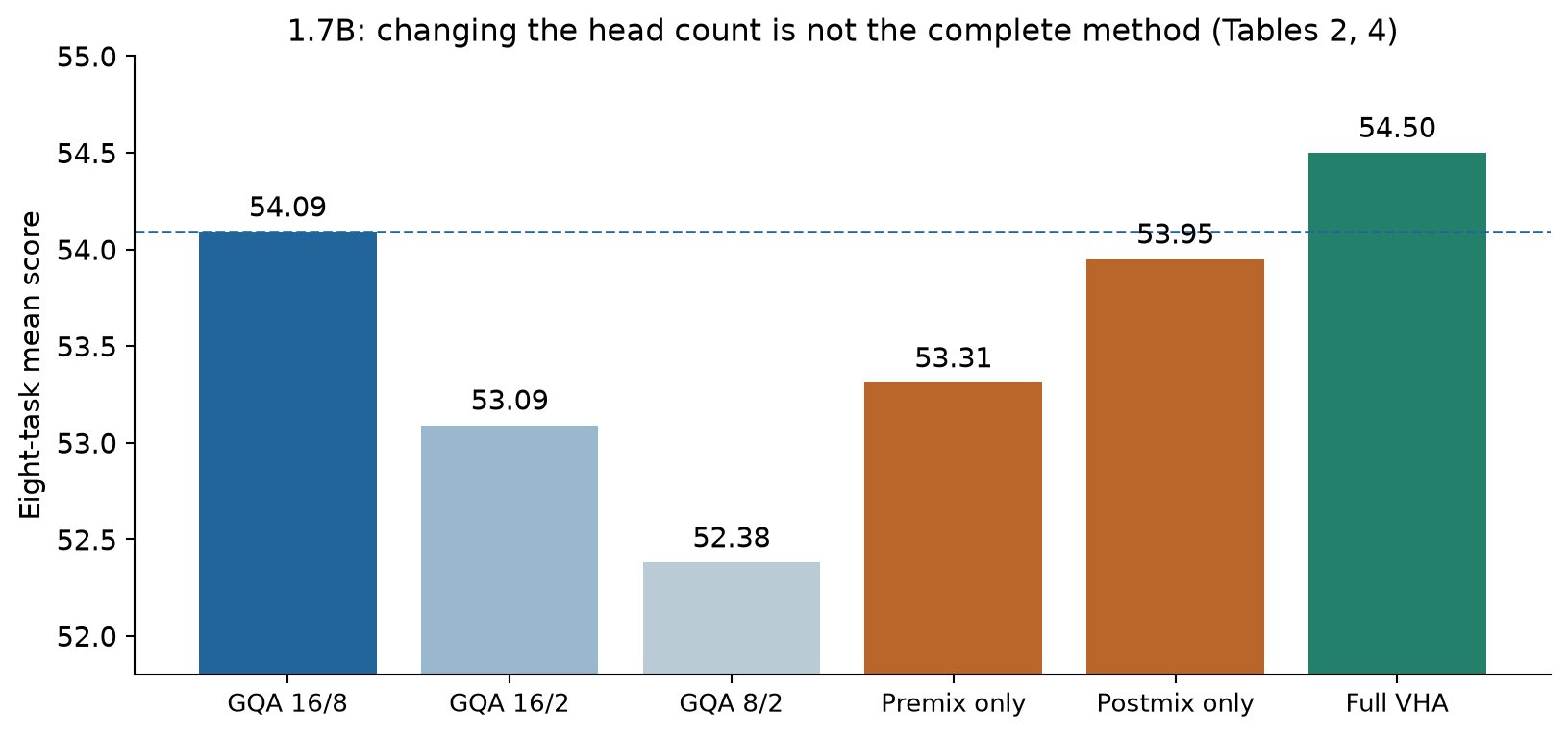
Table 2 is especially informative. Ordinary GQA with 16 query heads and 8 KV heads scores 54.09. Reducing KV heads to two while retaining 16 query heads gives 53.09. Reducing both to 8 query heads and 2 KV heads gives 52.38. VHA uses 8 physical query heads and 2 KV heads, but expands to 16 virtual attention heads, and scores 54.50.

The first low-cache comparison asks whether VHA training helps a two-KV-head inference architecture. The second shows why merely shrinking the physical projection is not the complete solution. It would be misleading to describe VHA and the 8-query-head baseline as having identical effective attention capacity: virtual expansion restores sixteen distributions. The larger query count is part of the method’s computation, even though its initial projection is shared.

Table 4 then separates Premix and Postmix. At 1.7B, Premix alone scores 53.31 and Postmix alone 53.95, versus 54.50 together and 54.09 for the GQA baseline. At 4B, the corresponding values are 56.62, 57.22, 57.71 and 56.90. The full design is strongest in both cases. But Postmix alone already beats the 4B baseline, so a statement that neither component ever helps on its own would be false.

7.3 Larger-scale evidence is useful but uses another training setting

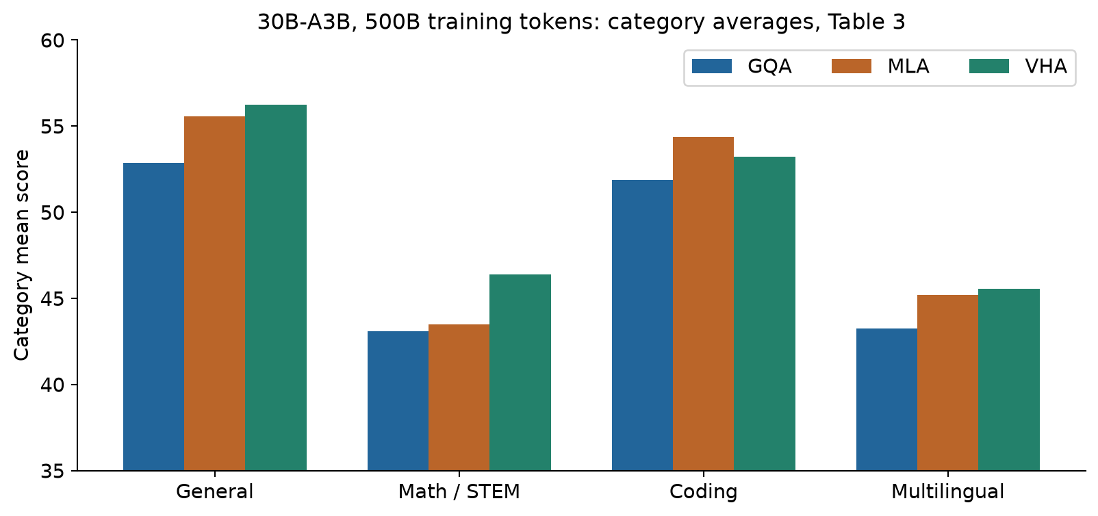
The 30B-A3B experiment uses an ERNIE-style MoE model, 500B tokens from an internal corpus, context length 8,192 and FP8 training. Its GQA configuration has 48 query heads and 4 KV heads; VHA has 24 physical queries, 48 virtual queries and 2 KV heads. Cache figures in the comparison use BF16 accounting. FP8 training precision should not be silently substituted into that cache formula.

Table 3 groups twelve benchmarks into four categories and then averages those category means. This is a category macroaverage, not an unweighted mean over twelve tasks. GQA, MLA and VHA obtain 47.76, 49.66 and 50.36 respectively. VHA improves by 2.60 points over GQA and 0.70 over MLA. Its coding category, however, is 53.23 versus MLA’s 54.37.

The detailed table explains why the aggregate needs context. VHA’s HumanEval+ score is 47.56, below GQA’s 50.00 and MLA’s 52.44, while its MATH score is 48.84, above 38.18 and 43.42. The result supports a favorable overall balance in this training configuration, but not uniform improvement. Because the corpus and architecture differ from the smaller experiments, one should not fit a simple scaling trend through all these scores.

7.4 Long-context gains come from a third experimental family

The long-context study uses a separate 10B-A1B model with a MiMo-2.5-Flash-style hybrid attention layout. One quarter of layers use full attention and three quarters use sliding-window attention. Only the full-attention modules receive the two-versus-four-KV-head change. Treating these measurements as a longer-context evaluation of the 30B model would conflate different experiments.

Training proceeds through an 8K stage with 500B tokens, then a 32K stage with 100B, and a 128K stage with another 100B. RoPE bases change across stages. At the final 128K checkpoint, the RULER overall scores at evaluation lengths 8K, 16K, 32K, 64K and 128K are 90.1, 88.5, 85.3, 81.3 and 76.8 for VHA, compared with 79.1, 78.2, 72.6, 69.5 and 65.7 for GQA. The mean difference across those lengths is about 11.4 points. [1, Table 6]

Variable tracking is an especially large contributor. At 128K, VHA scores 83.0 versus 3.0 for GQA. The benchmark has thirteen tasks; if the overall uses equal task weights, an 80-point gain on one task contributes roughly 6.15 points to the overall difference. That arithmetic does not invalidate the overall result. It identifies a specific capability that deserves closer investigation instead of treating the aggregate as a uniform improvement across all retrieval behaviors.

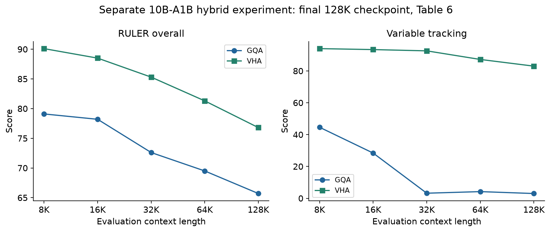
Other long-context benchmarks temper the picture. At the final checkpoint, LongBench-v2 is 24.2 versus 18.9 and BABILong is 38.2 versus 31.1, while InfiniteBench is 31.5 versus 31.8. HELMET categories favor VHA for retrieval-augmented generation, long QA and summarization, but not uniformly for in-context learning. The preceding 32K checkpoint is less favorable: LongBench-v2 is 22.3 for VHA versus 28.0 for GQA, and InfiniteBench is 27.3 versus 29.9. Stage dependence is part of the result, not a detail to omit after selecting the final checkpoint.

7.5 What the robustness appendix actually adds

Appendix B repeats 0.6B training in a different efficient training setup. Four VHA runs have a mean score of 50.40 with standard deviation 0.07; three GQA runs average 50.00 with standard deviation 0.34. This supports the small-scale ordering under repeated runs, while also showing that one GQA run, at 50.39, is close to the VHA mean. These scores should not be pooled with the main Table 1 scores because the training setting differs.

The initialization study compares default identity perturbation, a larger perturbation and fully random Premix. All remain numerically stable during the reported early 2,000-step check, while the default gives better downstream quality in that setup. This supports a useful initialization preference. It does not prove numerical instability for every alternative, nor establish that early stability guarantees a favorable final model.

8. Limitations and failure boundaries

The central limitation is the gap between an analytical resource advantage and a measured system advantage. The paper provides detailed FLOP estimates and cache formulas, but not a matrix of end-to-end prefill and decode measurements across batch sizes, sequence lengths, devices and export choices. Kernel compatibility makes adoption easier; it does not determine the magnitude of speedup. Very small KV-head counts may also interact with parallel work partitioning in ways that byte counts alone do not capture.

A second limitation is training coverage. The largest experiment uses 500B tokens, and the long-context study has a staged 700B-token curriculum. These are substantial experiments, but they do not establish behavior at much longer pretraining budgets, across all model families, or after extensive reinforcement learning. The paper itself leaves larger-scale training and combinations with quantization or sparse attention for future work. Existing evidence should not be stretched into a guarantee about those combinations.

Third, architecture comparisons involve multiple simultaneous choices. Matching approximate model size, cache bytes and training tokens does not necessarily match total FLOPs, optimizer state, expressivity or the best hyperparameters for each baseline. The controlled head-count and component ablations help, but they do not eliminate every alternative explanation. A parameterization that is favorable at one learning rate may lose its advantage after a baseline receives its own tuning budget.

Fourth, seed uncertainty is unevenly characterized. The appendix adds small-model repetitions, while the larger and long-context studies still lack a broad multi-seed account. A difference of 0.05 points and a difference of 11.4 points should not be discussed with the same confidence. Benchmark composition also matters: an overall average can be dominated by a few task types, and category macroaverages differ from per-task macroaverages.

Finally, exact algebraic folding has a precise domain. Constant learned linear matrices can be composed; nonlinearities, token-dependent mixing or an incorrect RoPE order generally break the simple argument. Finite precision introduces additional numerical questions. The paper establishes a deployable architecture and promising empirical results, not an unrestricted equivalence between all compressed and uncompressed checkpoints.

9. Critical analysis: the strongest explanation is about optimization

9.1 Redundant linear factors can change the learning trajectory

A standard dense output projection already combines information across attention heads. Postmix does not create the first opportunity for cross-head communication in the layer’s final output. Because its linear transform can be absorbed into $W_O$, it does not enlarge the unconstrained output projection’s linear function class. Its benefit must instead concern the route by which training finds an effective output matrix, the regularization imposed by the factors, or their interaction with the shared query design.

A simple derivation clarifies why forward equivalence does not imply training equivalence. Consider one product $F=WP$ and let $D=\partial\mathcal L/\partial F$. Under a simultaneous plain-SGD step of size $\eta$,

$$W_+=W-\eta DP^\top,\qquad P_+=P-\eta W^\top D. \tag{14}$$

Multiplying the updated factors gives

$$\begin{aligned} F_+={}&F-\eta\left(DP^\top P+WW^\top D\right)\\ &+\eta^2DP^\top W^\top D. \end{aligned} \tag{15}$$

This differs from the direct update $F-\eta D$. The factor norms and orientations transform the effective update. Shared factors in VHA add further coupling across heads. Equation 15 is an explanatory toy derivation, not the actual AdamW update used in the paper, and it does not prove improvement. It shows exactly why a richer training graph can matter even when export removes it.

9.2 Raw matrix differences are not a complete diversity measurement

The paper visualizes Premix matrices moving away from identity and differing across groups. Those observations are useful descriptions of the learned parameters, but factorized representations have a change-of-basis freedom. For any common invertible $T$,

$$W_i\longmapsto W_iT,\qquad P_g\longmapsto T^{-1}P_g \quad\Longrightarrow\quad W_iP_g\ \text{unchanged}. \tag{16}$$

Distances between raw factors can therefore change while every effective query projection remains identical. Weight decay and initialization can favor some factorizations, but they do not make raw factor distance a direct measure of functional diversity. Stronger evidence would compare effective query–key operators, attention distributions on matched inputs, and targeted interventions on the learned factors. This is a proposal for mathematical and experimental analysis, not a claim that new experiments were performed here.

Likewise, off-diagonal Postmix entries demonstrate that the learned residual mixes head coordinates. They do not by themselves show a new representational capacity unavailable to a dense output projection. The more interesting question is whether the low-rank branch offers a better-conditioned or better-regularized path to a useful final matrix.

9.3 The bottleneck sweep needs a rank cap

The paper tests $r=4,32,128$ at 1.7B and reports means of 54.50, 54.24 and 54.15. A larger bottleneck can lower training loss while worsening evaluation, which is consistent with a regularization interpretation. However, the residual matrix is only $16\times16$, so

$$\operatorname{rank}(BA^\top)\leq\min(r,16). \tag{17}$$

The $r=32$ and $r=128$ cases cannot produce residual ranks of 32 and 128. Both can represent a full-rank sixteen-head residual; they differ in overparameterization and optimization geometry. Calling this entire sweep simply “increasing the matrix rank” obscures that distinction. Seed repetitions and a sweep around $r=1,2,4,8,16$ would more cleanly separate a rank restriction from redundant factor width.

9.4 A folded model trades one convenience for another

VHA is particularly appealing if a model developer can change pretraining but wants a conventional serving graph. A deployment team receiving only an arbitrary existing checkpoint cannot obtain the same benefit by mechanically attaching and folding identity modules. Training has to exploit the shared factors and small KV representation first.

Even for a trained VHA model, the best graph may depend on workload. Folding removes extra operators and simplifies kernel integration, while retaining factors preserves the narrower physical query projection. The appropriate comparison is a measured Pareto curve over prefill latency, decode latency, batch capacity and numerical agreement. Reporting both paths would strengthen the systems case without weakening the architectural contribution.

The paper’s most durable contribution is this separation of training and inference parameterizations. The empirical advantage is plausible because the parameterization changes learning, not because matrix multiplication grants extra nonlinear capacity for free. Recognizing that makes the result more interesting and its boundaries easier to test.

10. Conclusion

VHA trains a two-KV-head attention layer through shared physical queries, group-specific linear expansion and a low-rank residual head mixer. It then folds those constant transformations into ordinary query and output projections. The result is a familiar GQA inference structure with a training history that differs from directly optimizing its final dense matrices.

The reported evidence supports a favorable cache–quality trade-off, modest reductions in estimated training FLOPs, and strong gains on some long-context retrieval tasks. It does not establish a measured two-to-fourfold end-to-end speedup, uniform improvement on every benchmark, or lossless conversion of arbitrary pretrained checkpoints. I would view VHA as a promising pretraining architecture whose next decisive evidence should connect its elegant folding argument to workload-specific system measurements and more controlled optimization studies.

References

1. Xibo Ding, Guoxia Wang, Jinle Zeng, Jiabin Yang, Sirui Tao, Chao Yang, Dianhai Yu. Virtual Head Attention, arXiv:2610.17959v1, 2026-10-13. Paper record · Reviewed full PDF · Full text. All reported VHA measurements in this review come from this version, including its appendices.
2. Official VHA resource, linked by the authors. Included as a resource entry point.