KV-CoRE: What Does the Rank of a KV Cache Actually Tell Us?

Review date: 2026-10-31 · Author: Zhongzhu Zhou
Paper reviewed: KV-CoRE: Benchmarking Data-Dependent Low-Rank Compressibility of KV-Caches in LLMs
Paper authors: Jian Chen, Zhuoran Wang, Jiayu Qin, Ming Li, Meng Wang, Changyou Chen, Yin Chen, Qizhen Weng, Yirui Liu
arXiv: 2602.05929 · Version: v2, 2026-02-07

1. A diagnostic question before a compression policy

A low-rank cache method needs an answer to a deceptively simple question: how many directions must be retained? A fixed rank can be wasteful in one layer and destructive in another. A rank selected on English instruction data can also behave differently on medical text, code, or another language. KV-CoRE studies this variation by measuring the singular spectra of the actual key and value activations produced by a model on a dataset.

This is primarily a diagnostic framework. It constructs data-dependent low-rank projections and tests the resulting degradation, but it does not establish an end-to-end serving speedup. Its main contribution is a structured way to compare representational concentration across layers, models, and datasets. The relevant question is not merely whether a cache can be made smaller, but whether a spectral summary identifies the settings in which doing so is less damaging.

The distinction from yesterday’s iS-KV reading is useful. iS-KV maintains a truncated representation while new token blocks arrive, updating the historical coordinates when the basis changes. KV-CoRE accumulates a full feature Gram matrix over a dataset and decomposes it at the end. Both use low-rank geometry, but their temporal responsibilities differ: an online approximation must manage information already discarded, whereas a dataset diagnostic can retain the complete second-order statistic needed for its final spectrum.

The paper reports several informative patterns. Keys often have more concentrated spectra than values. The rank profile varies by layer, and architectural KV width matters. Dataset-level normalized effective rank correlates with an aggregate measure of perplexity sensitivity, particularly for values. These results make spectra worth measuring. They do not turn normalized effective rank into an automatic rank selector, a guarantee of answer preservation, or a measurement of serving latency.

This review separates three levels of evidence: exact linear-algebra statements, numerical observations reported by the paper, and proposed follow-up experiments. All model results below come from the paper; the small analytic examples and table arithmetic are calculations in this review, not new model experiments. Reading the appendices also exposes reporting ambiguities that matter for interpretation, including inconsistent judge-model descriptions and several summary values that cannot be recovered from the visible table rows.

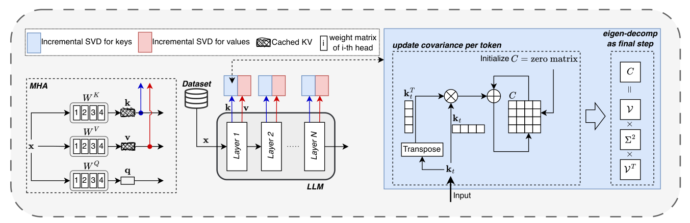
Figure 1. Cropped from paper Fig. 1, p. 3. The right panel accumulates outer products and performs an eigendecomposition at the end. This is the statistic behind the dataset-level spectrum. Source: Chen et al., arXiv:2602.05929v2, CC BY 4.0.

2. Prerequisites: what is being compressed?

2.1 The physical cache and the feature matrix

At one layer, let a sequence contain $L$ tokens, with $H_{kv}$ physical KV heads and head width $D$. Concatenating those heads gives a feature width $d=H_{kv}D$ and two matrices $K,V\in\mathbb R^{L\times d}$. A row denotes a token; a column denotes a feature coordinate. For a dataset, rows from multiple examples can be stacked for spectral analysis, even though examples remain separate causal sequences during model evaluation.

That distinction prevents an easy conceptual error. Combining rows to estimate a spectrum does not mean that tokens from unrelated prompts attend to each other. It means that one feature-space basis is estimated from a collection of activations. The weighting of examples is nevertheless important: stacking all tokens weights long examples more heavily unless a different sampling or weighting scheme is specified.

For one attention head, using already position-processed queries and keys, the calculation is

$$a=\operatorname{softmax}\left(\frac{qK^\top}{\sqrt D}\right),\qquad o=aV. \tag{1}$$

The cache avoids recomputing historical keys and values. It still has to be read during decoding. Reducing the number of cached scalars can relieve capacity pressure, but whether it reduces time depends on the representation, kernels, reconstruction, and batching. Storage accounting and latency accounting answer different questions.

If each cached scalar occupies $b$ bytes, a conventional cache for one sequence over $N_{\ell}$ equal-width layers uses approximately

$$M_{\mathrm{dense}}=2bN_{\ell}Ld. \tag{2}$$

The factor two counts keys and values. Real systems add allocation, alignment, and metadata costs. Grouped-query attention shares KV heads among multiple query heads; the correct width in this expression is the number of physical KV heads, not the larger number of query heads. Otherwise the baseline memory is overstated before any compression is considered.

2.2 Data-dependent activation compression versus weight compression

Write $K=XW_K$, where $X\in\mathbb R^{L\times d_e}$ contains hidden states and $W_K\in\mathbb R^{d_e\times d}$ is the projection. Compressing $W_K$ under its own Frobenius norm treats all input directions equally. Compressing the observed $K$ weights errors by the hidden states that actually occur.

For any weight perturbation $E=W_K-\widetilde W_K$, the activation error is

$$\|XE\|_F^2=\operatorname{tr}(E^\top X^\top XE). \tag{3}$$

Thus two weight approximations with the same $\|E\|_F$ can have very different effects on the data. A direction with large weight error may be almost unused; a small weight error may align with a frequently excited hidden-state direction. The matrix $X^\top X$ supplies this data-dependent geometry.

The benefit also defines the failure boundary. A basis fitted to one distribution is optimal only for the activations included in that objective. A new domain can activate neglected directions. The paper’s diagnostic is therefore most useful when the calibration distribution and its intended deployment distribution are described together, rather than when a single model-wide number is presented as an intrinsic property of the weights.

3. The exact optimization result, step by step

3.1 Truncated SVD solves a reconstruction problem

Let the nonzero singular values of $K$ be $\sigma_1\geq\cdots\geq\sigma_r>0$. A thin singular value decomposition is $K=U\Sigma B^\top$, where the columns of $U$ and $B$ are orthonormal. This review uses $B$ for the right singular vectors so they are not confused with the value cache $V$.

For a retained rank $k\leq r$, define $K_k=U_k\Sigma_kB_k^\top$. The Eckart–Young result gives

$$\min_{\operatorname{rank}(A)\leq k}\|K-A\|_F^2 =\|K-K_k\|_F^2 =\sum_{i=k+1}^{r}\sigma_i^2. \tag{4}$$

One way to understand this is to rotate the approximation into the singular-vector coordinates. Orthogonal changes of coordinates preserve Frobenius norm. In those coordinates, the matrix is diagonal and its squared energy is the sum of squared singular values. A rank-$k$ approximation can retain at most $k$ independent directions; retaining the largest singular values leaves the smallest possible discarded energy. The spectral-norm residual is separately $\sigma_{k+1}$.

This theorem is powerful because the objective is explicit. It says nothing about the importance of a discarded direction to a rare query, nor about errors accumulated when every layer is altered. The original matrix is the optimization target. Answer correctness is a different, downstream target.

3.2 The optimal activation projection can be realized through the weights

The paper proposes the data-dependent weight approximation

$$\widetilde W_K=W_KB_kB_k^\top. \tag{5}$$

Substituting it into the model projection gives the desired truncated activations:

$$\begin{aligned} X\widetilde W_K &=XW_KB_kB_k^\top \\ &=KB_kB_k^\top \\ &=U\Sigma B^\top B_kB_k^\top \\ &=U_k\Sigma_kB_k^\top=K_k. \end{aligned} \tag{6}$$

The third line uses orthonormality: multiplying by $B_k$ selects the first $k$ singular directions. Also, $\operatorname{rank}(W_KB_kB_k^\top)\leq k$. Consequently the approximation is feasible for a rank-at-most-$k$ weight constraint and attains the globally optimal rank-$k$ activation reconstruction error on this $X$. No training or gradient optimization is needed to establish that result.

The use of “at most” avoids a technical distraction when the data or weights are already rank deficient. There can also be multiple optimal weight matrices: components in the null space of $X$ do not change the observed activations. The theorem identifies an optimal construction, not necessarily a unique set of model weights.

3.3 What the factorization does not automatically buy

The factors $W_KB_k$ and $B_k^\top$ suggest caching $k$ coordinates per token. If one retains the reconstructed dense $K_k$ instead, there is no persistent-cache memory saving despite the low rank. If one stores coordinates but reconstructs a dense cache for every attention operation, the persistent footprint can fall while bandwidth, workspace, or latency remains unfavorable.

The head structure introduces a further constraint. KV-CoRE concatenates head features before finding a shared basis. A singular direction can therefore mix several physical KV heads. Standard attention expects separate head-specific key and value spaces and separate softmax distributions. A general cross-head projection does not automatically preserve that organization or fit an existing fused kernel.

A per-head or block-diagonal basis is an alternative. It is easier to align with the attention layout, but its feasible approximation set is smaller, so the unconstrained SVD optimality guarantee no longer applies at the same total rank budget. The joint spectrum is a useful diagnostic of available redundancy; realizing all of that redundancy efficiently may require a different architecture or a more constrained compression problem.

Positional transformations need the same care. If $R_t$ denotes a position-dependent rotation and $P=B_kB_k^\top$, then generally $R_tP\neq PR_t$. A projection estimated before rotary position encoding cannot simply be moved after it. A deployment proposal must state whether its feature matrix contains pre-rotation or post-rotation keys and explain how the positional path is represented. Appendix A’s discussion of decoupled positional components in latent attention is relevant background, not a proof that an arbitrary fitted SVD can be absorbed into any existing model.

4. Incremental computation: accumulate the Gram matrix

4.1 Why the full activation matrix is unnecessary

For $N$ dataset tokens, explicitly holding $K\in\mathbb R^{N\times d}$ can be expensive. Yet the right singular vectors and singular values can be recovered from a $d\times d$ matrix:

$$C=K^\top K=B\Sigma^2B^\top. \tag{7}$$

If $K$ is partitioned into row blocks $K_1,\ldots,K_T$, ordinary matrix multiplication yields

$$C=\sum_{t=1}^{T}K_t^\top K_t. \tag{8}$$

There are no cross-block terms: stacking rows and multiplying by the transpose on the left sums independent row outer products. For one row $k_t$, the update is $C\leftarrow C+k_t^\top k_t$. In practice a block matrix multiplication is more appropriate than a Python loop over individual tokens, but the mathematical statistic is the same.

After accumulation, diagonalize $C=B\Lambda B^\top$. Its eigenvalues satisfy $\lambda_i=\sigma_i^2$, so $\sigma_i=\sqrt{\lambda_i}$. This recovers the spectrum and right singular vectors without storing the left singular vectors or the entire dataset cache. It is exact in exact arithmetic as long as the full Gram matrix is retained.

Algorithm 1. Dataset spectrum and a rank-k projection

The following pseudocode expresses the mathematical procedure; numerical tolerances are decisions that must be recorded with the result.

Input: frozen model, dataset batches, layer/path, retained rank k
1. Initialize C as a d-by-d zero matrix in accumulation precision.
2. For each batch, run the frozen model and collect valid KV rows A.
3. Exclude padding and select the documented representation locus.
4. Update C <- C + transpose(A) * A; then release A.
5. Symmetrize C <- (C + transpose(C)) / 2.
6. Eigendecompose C; sort eigenpairs by descending eigenvalue.
7. Check negative eigenvalues against a numerical tolerance.
8. Set justified roundoff-scale negatives to zero; take square roots.
9. Record the numerical-rank rule, spectrum, and effective rank.
10. Retain B_k; return W * B_k and transpose(B_k) if needed.
Output: dataset spectrum, diagnostic metrics, projection factors

The paper calls this incremental SVD. The important operational detail is that its displayed algorithm updates the Gram statistic and decomposes at the final step. It does not repeatedly truncate a moving basis after every token. Replacing it with a rank-limited streaming sketch could reduce cost, but would change the exactness claim and introduce approximation error into the diagnostic itself.

4.2 Time, memory, and numerical conditioning

Accumulating $N$ rows costs approximately $O(Nd^2)$ arithmetic, followed by $O(d^3)$ for a dense eigendecomposition. Persistent storage is $O(d^2)$ plus a batch buffer. This scales well with dataset length compared with retaining all activations, but the quadratic dependence on feature width can be significant.

As illustrative accounting, one FP32 Gram matrix at $d=1024$ occupies 4 MiB; at $d=4096$ it occupies 64 MiB. Retaining both key and value matrices for 32 layers at the latter width requires 4 GiB just for those statistics. At $d=256$, the corresponding single matrix is 0.25 MiB. These are storage calculations, not measured memory peaks from the paper. Processing layers in groups can trade model passes for lower simultaneous storage.

The paper uses the word covariance, but the displayed statistic is the uncentered second moment $K^\top K$. Subtracting a feature mean would change the spectrum and the approximation objective. If a centered decomposition is desired, the mean has to be stored and reconstructed as part of the representation; it is not an innocuous preprocessing substitution.

Gram construction also squares the condition number of a full-rank matrix. Very small singular directions can become numerically difficult to distinguish from zero. A numerical-rank threshold therefore affects both the spectrum tail and the denominator of normalized effective rank. Accumulation precision, eigenvalue tolerances, and normalization choices should accompany comparisons. Clamping tiny negative eigenvalues caused by roundoff is reasonable; silently clamping a large negative value would conceal an invalid numerical result.

5. Normalized effective rank: useful, but not a budget

5.1 From a spectrum to an entropy

Given the nonzero singular values, KV-CoRE normalizes their magnitudes into a probability distribution and computes its entropy:

$$p_i=\frac{\sigma_i}{\sum_{j=1}^{r}\sigma_j},\qquad H=-\sum_{i=1}^{r}p_i\log p_i. \tag{9}$$

Exponentiating entropy gives the effective rank, and dividing by matrix rank gives the paper’s normalized effective rank:

$$\operatorname{erank}(K)=\exp(H),\qquad \operatorname{NER}(K)=\frac{\exp(H)}{r}. \tag{10}$$

The definition uses singular values, not squared singular values. If the calculation begins with eigenvalues of $C$, the square root must be taken before forming $p_i$. Normalizing eigenvalues directly would produce an energy-entropy statistic with a different numerical meaning.

For a flat spectrum with $r$ equal nonzero values, each $p_i=1/r$, so $H=\log r$, effective rank is $r$, and NER is one. If almost all mass concentrates in one singular value while the other $r-1$ remain positive, entropy approaches zero, effective rank approaches one, and NER approaches $1/r$. Thus NER summarizes how evenly the nonzero directions share singular-value mass.

Multiplying the entire matrix by a nonzero scalar does not change $p_i$. Orthogonal changes of feature coordinates do not change singular values. NER is consequently insensitive to overall scale and orthogonal orientation. This is attractive for comparing spectral concentration, but it also means the statistic discards information that can affect downstream error.

5.2 The denominator creates a real interpretive trap

Consider three analytic examples, shown in Figure 2. Eight equal singular values give effective rank eight and NER one. The spectrum $(12,1,1,1,1,1,1,1)$ gives effective rank about 3.96 and NER about 0.494. A matrix with exactly two equal nonzero singular values and six zeros has effective rank two, but its actual rank is two, so its NER is again one.

The third matrix can be represented exactly with two dimensions even though NER is maximal. This is not a contradiction: NER measures flatness relative to the nonzero rank. It is not normalized by ambient feature width unless actual rank equals that width. A high NER alone cannot distinguish a broadly used 1,024-dimensional space from a perfectly flat two-dimensional subspace.

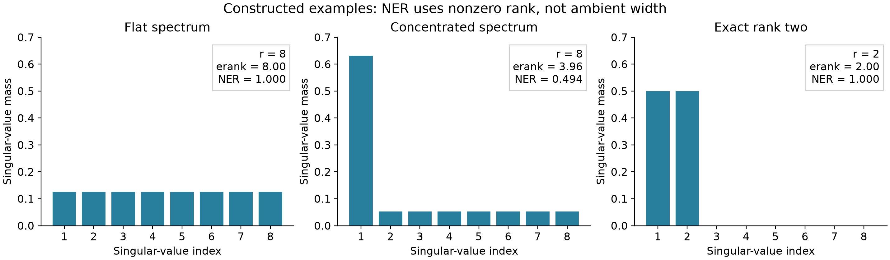
Figure 2. Original analytic illustration. Zero singular values are excluded from the rank denominator. The rank-two example shows why NER must be reported with actual or numerical rank and ambient width. These are constructed matrices, not model measurements.

This also creates sensitivity near a rank threshold. Adding an arbitrarily small nonzero direction can increase the mathematical rank while barely changing entropy. In floating-point work, different thresholds can therefore change NER appreciably even when the dominant spectrum is nearly identical. A numerical convention is unavoidable; silently changing that convention across models is not.

The zero matrix is a separate edge case. Both the singular-value normalization and the rank denominator are undefined. Assigning it NER zero might be a practical reporting convention, but it must be identified as a convention rather than an evaluation of Equation 10.

5.3 NER is different from retained energy

The Frobenius truncation objective depends on squared singular values. A natural reconstruction diagnostic at budget $k$ is the relative residual

$$\epsilon_F^2(k)=\frac{\sum_{i>k}\sigma_i^2}{\sum_{i=1}^{r}\sigma_i^2}. \tag{11}$$

NER compresses a whole spectrum into one entropy number; Equation 11 describes a budget-dependent tail. Different spectra can share similar entropy but place different amounts of energy beyond a specific rank. There is no general rule that a cache with NER 0.4 should retain exactly 40% of its width.

A useful diagnostic report therefore includes at least the ambient width, numerical rank, effective rank, NER, and a tail-energy curve. The entropy number helps organize comparisons. The curve answers the more operational question of what reconstruction loss a proposed budget incurs. Neither by itself certifies task quality, but keeping both prevents an avoidable loss of information.

6. Experimental design and metric semantics

6.1 What is compared

The paper examines Qwen3-4B and Qwen3-8B, Mistral-7B, Gemma-1.1-2B and 7B, Phi-3-mini-128k, and LLaMA-2-7B in its main table. The five English datasets are Alpaca, MedAlpaca, CodeAlpaca, WizardCoder, and FunctionCall. Its multilingual analysis uses query text from VisRBench. The intended coverage is fifteen non-English languages alongside English.

The document’s coverage descriptions are not completely consistent. The model paragraph does not enumerate LLaMA-2 although the table evaluates it. The language list includes Danish, while the displayed multilingual portion of Table 1 contains fourteen language rows and no Danish row. These discrepancies do not invalidate the visible measurements, but they prevent treating the prose counts as a complete inventory of the reported results.

The experiments are gradient-free. The model produces activations and is then evaluated under SVD-based truncation. The hardware description mentions a server with eight A800 80 GB GPUs and says evaluations use a single GPU. This establishes the experimental environment; it is not evidence of multi-GPU speedup or a serving throughput improvement.

6.2 Perplexity measures predictive likelihood

For a fixed tokenized evaluation sequence, perplexity is the exponential of average negative log likelihood:

$$\operatorname{PPL}=\exp\left[-\frac{1}{T}\sum_{t=1}^{T} \log p(x_t\mid x_{<t})\right]. \tag{12}$$

It measures how well the model predicts observed tokens under that evaluation protocol. It is sensitive to tokenization, text distribution, and the tokens included in the loss. Comparing compressed and uncompressed versions of the same model on the same examples is much easier to interpret than comparing absolute PPL across unrelated tokenizers or languages.

PPL also does not directly measure the quality of free-running generated answers. During likelihood evaluation, the context is typically the reference sequence. During generation, one changed token alters subsequent inputs. Small average likelihood changes can coexist with noticeable differences in reasoning trajectories or answer usefulness.

6.3 ND-PPL averages pairwise degradation, not only baseline degradation

Let $P(k,v)$ denote perplexity at retained key and value ranks $k$ and $v$. The paper’s key-side aggregate averages relative changes over less-to-more compressed key pairs and over value settings. An equivalent compact expression is

$$\operatorname{ND\!PPL}_K= \frac{1}{|\mathcal V|\,|\mathcal P_K|} \sum_{v\in\mathcal V}\sum_{(k_i,k_j)\in\mathcal P_K} \frac{P(k_j,v)-P(k_i,v)}{P(k_i,v)},\quad k_i>k_j. \tag{13}$$

Here $\mathcal P_K$ contains the ordered pairs with the larger retained rank first. The value-side metric is defined analogously. The denominator is the less-compressed member of each pair, not always the full-cache baseline. This matters when comparing the metric with a conventional percentage increase over the original model.

The aggregate depends on the chosen rank grid. Adding many aggressive settings can change it substantially, even when a practically relevant operating point is untouched. Perplexity can also vary non-monotonically, making some pairwise terms negative. A large aggregate should be interpreted alongside the surface from which it was computed, especially when the lowest value-rank settings produce extreme outliers.

Algorithm 2. Evaluate a fitted projection without hiding distribution shift

This is a proposed evaluation protocol extending the paper’s diagnostic; the held-out and paired checks below are recommendations, not claims about additional experiments performed by the authors.

Input: calibration split, disjoint test split, model, rank grid
1. Fit key/value bases per layer using calibration activations only.
2. Freeze those bases and all numerical-rank conventions.
3. Evaluate the full model on the same test examples as the reference.
4. For each key/value rank pair, evaluate likelihood and generation.
5. Record tail energy, PPL, answer metrics, and actual memory costs.
6. Compute pairwise ND-PPL using an explicitly saved rank grid.
7. Repeat on held-out domains/languages without refitting the bases.
8. Compare against a refitted-basis result to isolate adaptation value.
9. Report paired uncertainty and the exact judge prompt/model if used.
Output: in-distribution tradeoff, shift sensitivity, systems evidence

The separation in steps 1 and 7 matters because fitting and testing a basis on the same distribution answers an easier question than deploying a fixed basis under shift. The paper’s data-dependent construction is sound for its stated objective, but the published description does not fully resolve all calibration-versus-evaluation split choices. Those choices should remain an uncertainty, rather than being filled in by assumption.

7. What the spectra reveal across models and layers

7.1 Keys and values should receive separate budgets

On Alpaca, Table 1 reports key/value NER pairs of 0.428/0.724 for Qwen3-4B, 0.452/0.753 for Qwen3-8B, 0.612/0.900 for Gemma-2B, 0.359/0.469 for Gemma-7B, 0.449/0.773 for Mistral-7B, 0.409/0.616 for Phi-3, and 0.023/0.464 for LLaMA-2-7B. Within these displayed pairs, key spectra are more concentrated than value spectra.

This suggests that forcing equal retained ranks for keys and values is not obviously efficient. The two paths also play different functional roles: keys influence attention weights, whereas values carry the content combined by those weights. Spectral concentration provides a reason to investigate asymmetric budgets, but the final choice should depend on end-to-end quality and cost. A small key direction can still be decisive for a particular query.

The architecture comparisons need physical dimensions. The paper describes Gemma-7B with sixteen KV heads of width 256, giving $d=4096$, versus one width-256 head in Gemma-2B. A lower normalized rank in the larger space can coexist with a larger absolute number of useful directions. Qwen3-4B and 8B instead share a much closer KV configuration, with eight heads of width 128. Parameter count alone is therefore an inadequate explanation of the observed NER differences.

The English-domain results are fairly stable for some models, but not uniformly so. Qwen3-4B’s key entries across the five displayed English rows range from 0.421 to 0.432. LLaMA-2-7B ranges from 0.023 to 0.265. A conclusion that domains barely matter for every model would erase an important exception in the table itself.

7.2 The layer profile is a measurement, not a universal template

Figure 3 shows Qwen3-4B’s layerwise NER. Values tend to lie above keys, and the datasets often trace similarly shaped profiles. There are conspicuous local peaks and troughs. The model does not simply transition from low to high rank in a monotonic sequence, and one global compression ratio ignores that heterogeneity.

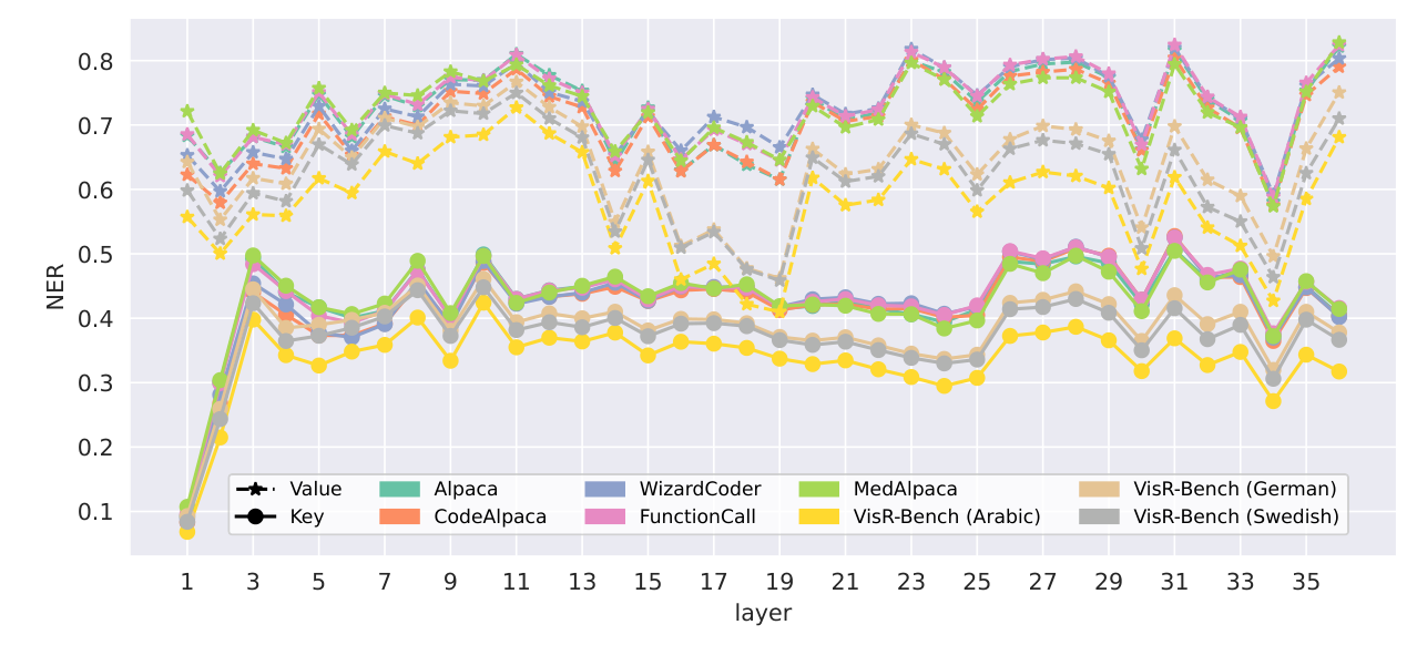
Figure 3. Cropped from paper Fig. 2, p. 8. Solid key curves and dashed value curves share architecture-dependent structure, with dataset-specific shifts. Source: Chen et al., arXiv:2602.05929v2, CC BY 4.0.

The appendix strengthens the point that layer allocation should be measured for the specific model. Its Qwen3-8B, Mistral, Phi-3, and Gemma plots have different shapes. In particular, Phi-3’s profile rises through much of the network, while the Gemma models show pronounced local variation. “The middle layers need more rank” is a possible summary of some curves, not a model-independent allocation algorithm.

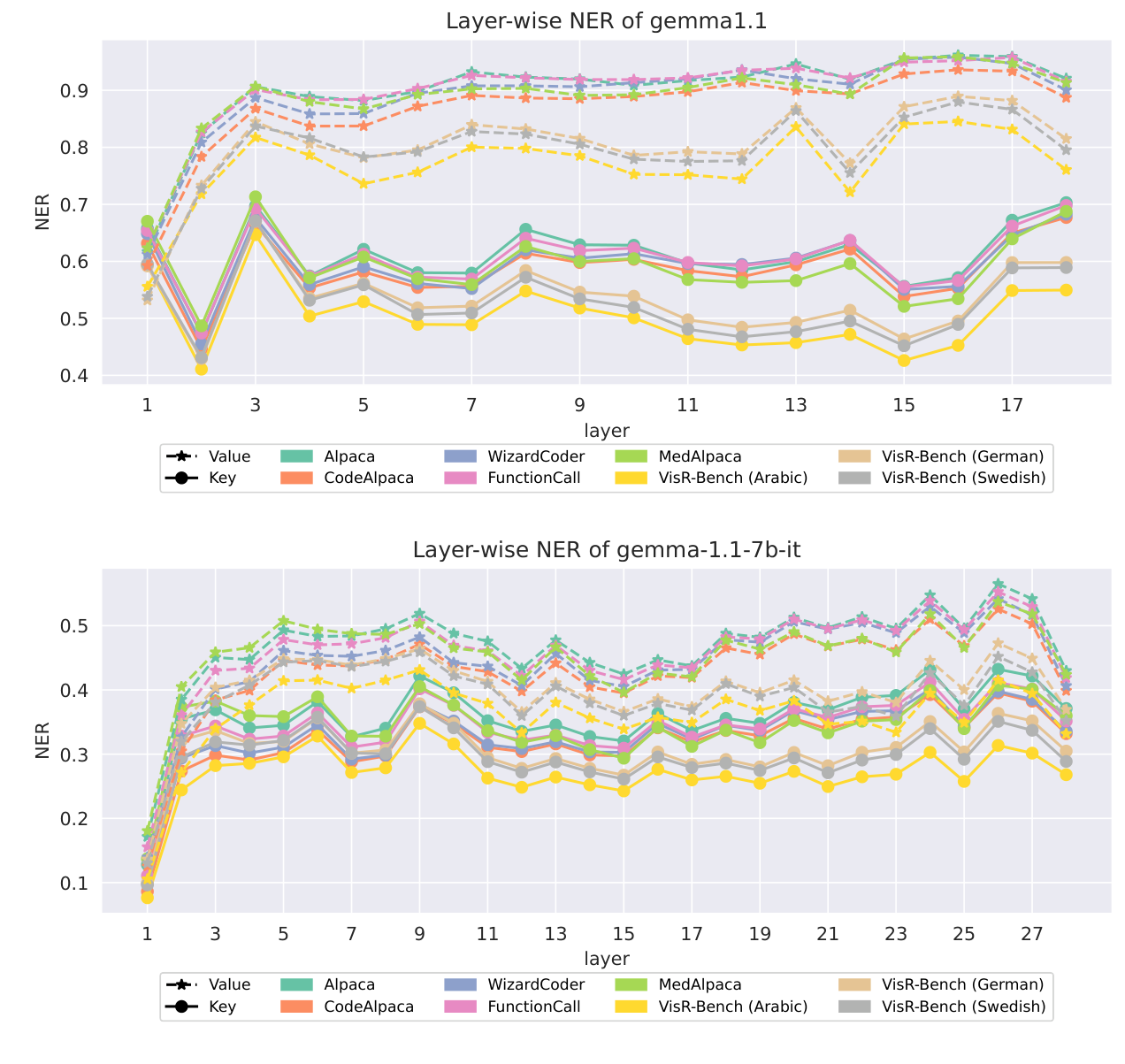
Figure 4. Cropped from paper Fig. B.3, p. 16. The two Gemma variants have different absolute NER ranges and layer patterns. Their KV feature widths also differ, so normalized rank alone is not a memory budget. Source: Chen et al., arXiv:2602.05929v2, CC BY 4.0.

If a total storage budget is available, a reconstruction-based allocation could compare the next retained singular direction in each layer: adding one direction reduces squared residual by that direction’s $\sigma^2$. However, directions have different storage costs when sequence lengths, widths, or layouts differ, and equal activation error across layers does not imply equal output sensitivity. This allocation idea is an analytic extension, not an algorithm validated by KV-CoRE.

7.3 Language variation and the limits of the coverage hypothesis

For Qwen3-4B, the visible multilingual key NER entries run from 0.337 for Arabic to 0.383 for Czech and German; corresponding value entries include 0.582 for Arabic and 0.640 for German. The paper interprets lower effective rank in some languages as possibly reflecting weaker representational coverage.

That is a plausible hypothesis, but the observation alone cannot identify its cause. Prompt length, tokenization, topic distribution, repeated templates, and the sampling of query text can all change an activation spectrum. Lower rank might indicate narrower input diversity rather than deficient language understanding. Establishing a training-data-coverage explanation would require matched data, independent proficiency measurements, and controlled comparisons.

There is also no general rule that the easiest distribution to compress is the one on which the model performs best. If an underused representation is low dimensional, compression may cause a small additional change to an already weak model. A diagnostic should therefore pair compression sensitivity with the uncompressed model’s quality, so that preserving poor behavior is not mistaken for successful capability retention.

8. From a low-rank cache to actual model behavior

8.1 Reading the perplexity surface correctly

Figure 5 varies retained key rank vertically and retained value rank horizontally. Larger ratios retain more dimensions. For Qwen3-4B on Alpaca, the full/full point has PPL 8.72. At 0.55/0.55, PPL is 10.69, an increase of approximately 22.6% calculated from those reported cells. LLaMA-2-7B moves from 6.04 to 6.30 at the same nominal ratios, approximately 4.3%.

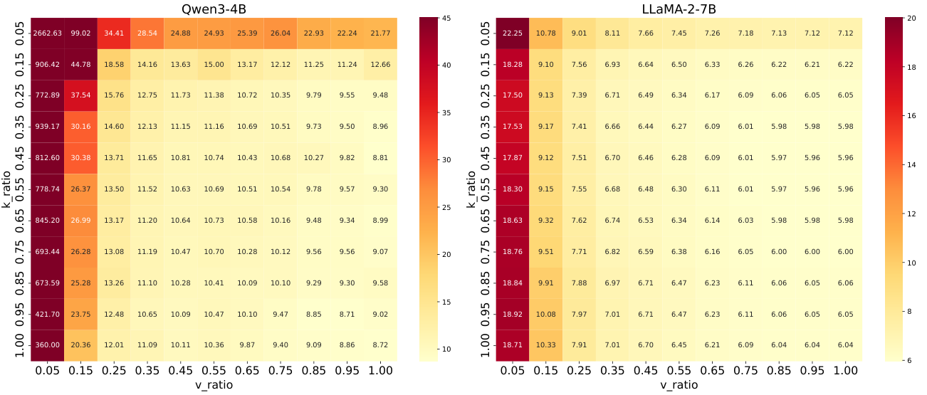
Figure 5. Cropped from paper Fig. 3, p. 8. Numerical cell labels must be read with the color scale: extreme Qwen values exceed the plotted color range. The two model panels also use different color limits. Source: Chen et al., arXiv:2602.05929v2, CC BY 4.0.

The asymmetry is substantial at the aggressive edge. Qwen3-4B with full key rank and value ratio 0.05 has PPL 360.00; with key ratio 0.05 and full value rank it has 21.77. With both ratios 0.05 the value reaches 2662.63. In LLaMA-2-7B, the corresponding three cells are 18.71, 7.12, and 22.25. These figures support separate treatment of K and V and explain why extreme value compression can dominate an aggregate sensitivity statistic.

Two cautions prevent overreading the comparison. First, equal retained fractions across models do not imply equal bytes, equal basis overhead, or equal absolute rank. Second, the heatmaps are not perfectly monotonic. Small improvements relative to a neighboring point may reflect evaluation variation or an incidental regularizing effect. They are not a reason to infer that throwing away more information universally improves the model.

8.2 Answer equivalence is a stricter test than mild PPL change

The paper additionally evaluates generated responses on 100 Alpaca instructions with a binary judge score. Figure 6 reports an average of 0.57 for Qwen3-4B at retained ratios 0.55/0.55, and 0.61 for LLaMA-2-7B. The latter is especially instructive: a roughly 4.3% increase in PPL accompanies only 61% judged equivalence under the paper’s protocol.

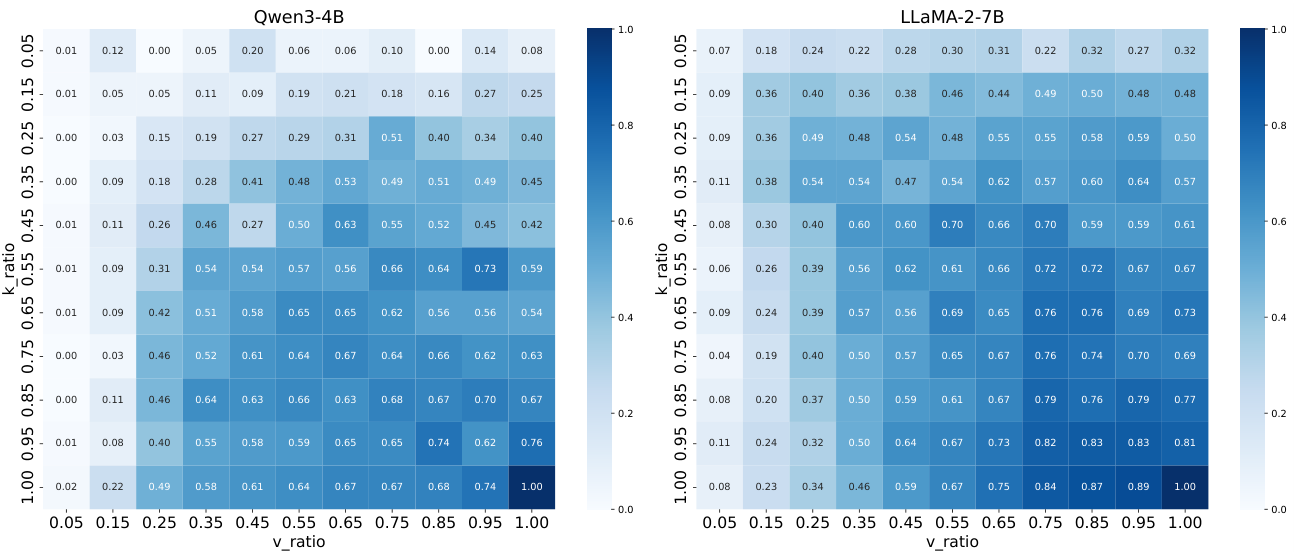
Figure 6. Cropped from paper Fig. 4, p. 9. A cell is the mean of binary judgments, not a continuous accuracy score. The full/full corner is 1.00; moderate truncation can visibly change generated answers. Source: Chen et al., arXiv:2602.05929v2, CC BY 4.0.

This does not mean that 39% of the compressed answers are objectively wrong. The judge compares quality against the full model according to a prompt, and the reference model is not an oracle. It does mean that near-baseline likelihood is insufficient evidence of response preservation. The two metrics illuminate different failure modes and should not be substituted for one another.

The judge description needs clarification before small differences can be trusted. Section 3.3 names GPT-4o and then GPT-5 in the same explanation. Appendix C also contains two rules whose priority is unclear: poor responses on both sides can count as equivalent, while the compressed response is elsewhere required to be reasonable. A precise model identifier, consistent rubric, generation settings, and repeated or paired uncertainty estimates would materially improve interpretability.

For scale, a binary proportion measured on 100 independent items has a maximum standard error of 0.05, giving a rough normal 95% interval of about plus or minus 0.10 near one-half. This is only an illustrative sampling calculation, not a confidence interval supplied by the authors; item dependence, repeated comparisons, and judge variability can add further uncertainty. Differences of one or two percentage points in this heatmap should consequently not be treated as decisive rankings.

8.3 Correlation is encouraging, but it is not a calibrated controller

Figure 7 connects dataset-level NER with ND-PPL for Qwen3-4B. The reported Pearson correlations are 0.88 for values and 0.64 for keys. A more dispersed spectrum is associated with greater degradation across the sampled compression settings, which is consistent with the intuition behind the diagnostic.

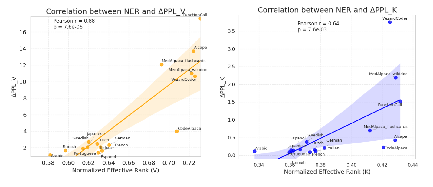
Figure 7. Cropped from paper Fig. 5, p. 9. The plots concern one model across datasets. The fitted association should not be read as a universal cross-model rank policy or a causal statement about language coverage. Source: Chen et al., arXiv:2602.05929v2, CC BY 4.0.

A useful next step would predict degradation on held-out datasets or models, with rank and architecture included as covariates. That would test whether the statistic generalizes as a decision aid rather than merely describing the samples from which the relationship was observed. A fitted correlation on the displayed points does not provide such a test.

The distinction is particularly relevant to the value-side correlation. ND-PPL aggregates a grid that includes very aggressive truncation. A predictor of catastrophic behavior at the extreme may be less informative about small quality differences near a deployment threshold. Reporting correlation separately for mild, moderate, and severe rank reductions would show which decision region the metric actually helps.

9. Why reconstruction optimality does not preserve attention

9.1 Follow the error through the operation

Let the approximate caches be $\widehat K=K+\Delta K$ and $\widehat V=V+\Delta V$ for a single head and a fixed query. The attention-logit perturbation is

$$\Delta s=\frac{q\Delta K^\top}{\sqrt D},\qquad \|\Delta s\|_2\leq\frac{\|q\|_2\|\Delta K\|_2}{\sqrt D}. \tag{14}$$

Even a relatively small cache residual can matter if a query aligns with it. Frobenius-optimal compression averages squared errors over rows and features; the future query determines which of those errors enters the logits.

For $a=\operatorname{softmax}(s)$, the Jacobian is $J=\operatorname{diag}(a)-aa^\top$. Its spectral norm is at most one-half. Integrating the Jacobian along the segment between two logit vectors gives

$$\|\widehat a-a\|_2\leq\frac12\|\Delta s\|_2. \tag{15}$$

This is a general worst-case bound for a fixed query. It does not exploit the actual attention distribution and can be loose. It nevertheless makes clear which intermediate quantities are relevant: query magnitude and direction, key residual, and softmax sensitivity.

The output difference can be decomposed without approximation:

$$\widehat o-o=(\widehat a-a)V+\widehat a\Delta V. \tag{16}$$

Consequently,

$$\|\widehat o-o\|_2 \leq\|\widehat a-a\|_2\|V\|_2 +\|\widehat a\|_2\|\Delta V\|_2. \tag{17}$$

Keys affect the weighting of values; value errors enter directly after weighting. The two terms interact, and subsequent layers change their queries as the hidden states change. A one-layer reconstruction guarantee is therefore neither an end-to-end error bound nor a task-preservation guarantee. The derivation is an explanatory analysis in this review, not a theorem claimed by KV-CoRE about full-model behavior.

9.2 What a useful rank policy would have to add

A practical controller needs a target: maximum quality loss, memory limit, or latency objective. NER alone specifies none of them. One possible sequence is to inspect NER for broad concentration, inspect tail energy for candidate ranks, test task sensitivity at those ranks, and then measure the actual serving implementation. Each stage removes a different uncertainty.

A query-weighted reconstruction objective could be closer to attention-logit fidelity than unweighted Frobenius error. A head-constrained basis could be closer to kernel compatibility. An online adaptive basis could reduce distribution mismatch. These are meaningful alternatives, but each changes the problem and has costs: extra calibration, reduced approximation freedom, or basis-update overhead. The clean diagnostic theorem should not be transferred to them without re-deriving the relevant guarantee.

For a single matrix stored as coordinates and a basis, a rough factor count is $Lk+dk$ versus $Ld$ dense scalars. Saving storage requires

$$Lk+dk<Ld \quad\Longleftrightarrow\quad k<\frac{Ld}{L+d}. \tag{18}$$

This illustrative formula includes a sequence-specific basis. A fixed basis shared across requests can amortize its cost differently. Either way, the shortcut “retained rank fraction equals memory fraction” misses an overhead term. At short contexts, that term can dominate. At long contexts, coordinates dominate, but reconstruction workspace and computation may still determine whether the representation is useful.

10. Limitations of the present evidence

The first limitation is scope. The diagnostic measures the low-rank structure of activations from selected models and datasets. It does not cover every architecture, serving workload, or long-context reasoning regime. A dataset-level spectrum can hide example-level outliers, including rare retrieval tokens or language switches that matter disproportionately to users.

The second limitation is the surrogate objective. Frobenius reconstruction treats all entries according to squared magnitude. It ignores the future query distribution, downstream sensitivity, and semantic importance of particular tokens. The paper’s perplexity and judge experiments partially bridge this gap, but do not eliminate it.

The third limitation is numerical and statistical specification. Rank thresholds, token weighting, split design, and the precise judge setup influence reproducibility and interpretation. The reported associations are useful observations, but they are not a calibrated out-of-distribution guarantee. A single scalar NER also loses the detailed shape of the truncation curve.

The fourth limitation is systems evidence. The paper supplies a memory-efficient way to collect spectra relative to storing all activations, and a mathematical low-rank construction. It does not report an end-to-end serving speedup demonstrating that arbitrary fitted bases reduce total latency. Persistent cache bytes, peak workspace, prefill time, decode time, and throughput should remain separate measurements.

Finally, the dataset-coverage interpretation is observational. Lower NER in a language does not by itself prove undertraining, and lower degradation under compression does not establish strong baseline capability. The diagnostic becomes more informative when paired with independent language-quality and input-diversity measurements.

11. Critical analysis: what should be trusted, and what needs repair?

11.1 Preserve the mathematics, narrow the operational claim

The strongest part of KV-CoRE is the connection between a data-dependent activation objective and a tractable full Gram statistic. Equation 6 makes the optimal projection construction explicit; Equation 8 explains how to recover its spectrum without retaining all token rows. Those claims survive the experimental reporting issues because they can be checked directly as matrix identities.

The operational interpretation should be narrower. Spectral concentration is evidence of reconstructive redundancy. It is not evidence that an arbitrary retained rank is safe, that language coverage caused that concentration, or that a factorized cache will be faster. The framework is valuable precisely as an early diagnostic in a larger decision process.

11.2 Table summaries need reconciliation with the displayed rows

A concrete arithmetic check reveals discrepancies in Table 1. For Qwen3-4B, averaging the five visible English key entries gives 0.4270, while the printed Average entry is 0.424. The corresponding value mean is 0.7224, versus printed 0.717. Those differences are larger than ordinary rounding of three-decimal inputs would explain.

For LLaMA-2-7B, the five English key entries average to 0.1254, versus the printed 0.088. The value entries average to 0.3728, versus printed 0.141. More strongly, 0.141 is below every one of the five displayed value entries, so it cannot be any nonnegative weighted average of just those rows.

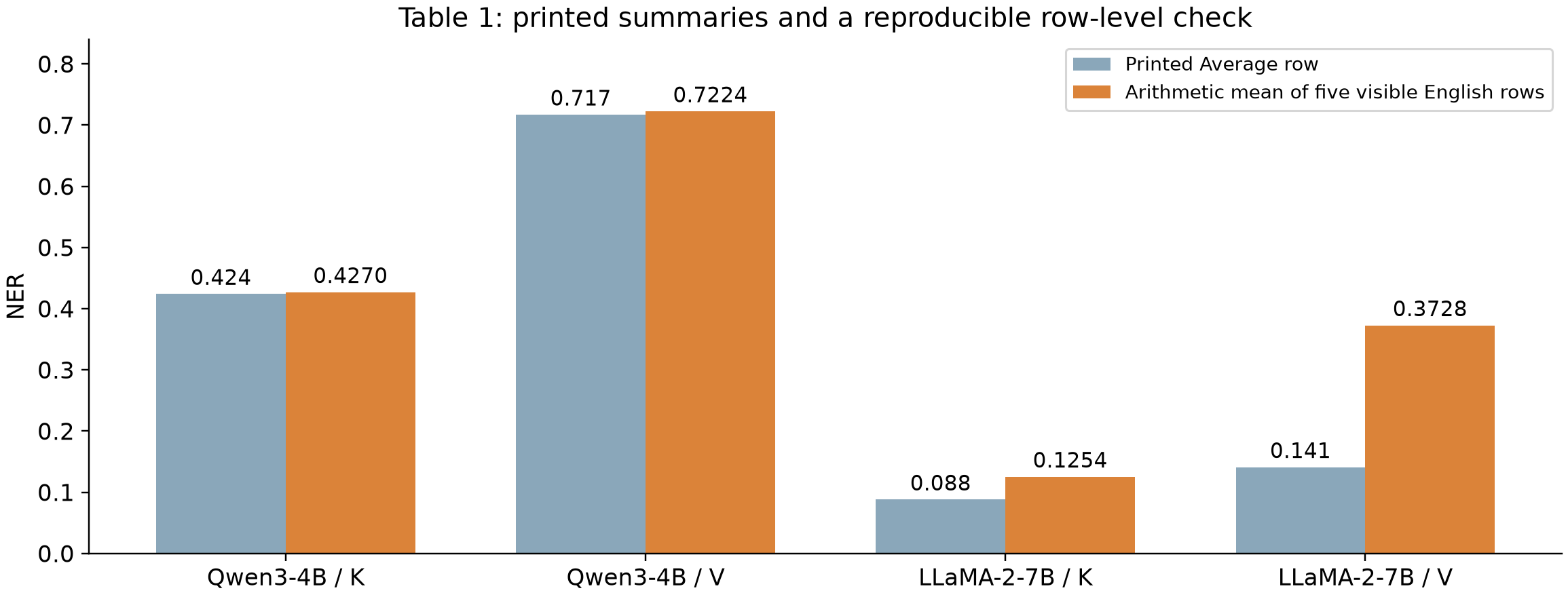
Figure 8. Original arithmetic using paper Table 1, p. 7. The orange bars are simple means of the five displayed English dataset rows; the blue bars reproduce the printed Average row. This identifies a reporting inconsistency and does not replace or re-estimate the underlying model measurements.

There is a similar problem in the visible Qwen3-4B multilingual summary. The printed key average is 0.387 although every displayed language key entry is at most 0.383; the printed value average is 0.653 although every displayed value entry is at most 0.640. An omitted population or a different aggregation procedure could potentially explain a different statistic, but the table does not make such a procedure clear.

The appropriate response is to rely on explicitly identified row-level values and label the summary discrepancy. It would be unjustified either to discard the entire study because of it or to silently substitute a guessed corrected table. A revised table with its complete population and weighting rule would resolve the issue directly.

11.3 Separate diagnostic validation from a coverage story

The correlation plots support testing NER as a compression-sensitivity feature. They do not establish that training coverage is the causal mediator. A stronger study would match token counts and text genres across languages, report tokenizer-dependent length differences, and compare baseline capability with compression sensitivity.

A particularly useful design would fit bases on one distribution and evaluate both the original and compressed models on another. Comparing that result with a basis refitted on the target distribution would separate transfer failure from intrinsic target-domain compressibility. It would also tell us when an online method such as iS-KV offers value beyond a fixed dataset projection.

11.4 Improve the quality comparison before ranking close settings

The judge-model naming inconsistency and rubric ambiguity deserve correction before the binary heatmap becomes a ranking benchmark. The reported 100-item sample is sufficient to show large degradations, but small differences need paired comparisons, repeated judgments or an independent task metric, and a clearly specified generation protocol.

The full model should remain a reference behavior, not a correctness oracle. An approximation may sometimes improve an answer or preserve an equally poor answer. A quality evaluation should distinguish correctness, usefulness, and equivalence rather than assume that any change is harmful or that any match is good.

11.5 The most useful extension is a budget-to-quality map

A deployment-oriented successor should report how NER, numerical rank, tail energy, head constraints, and query sensitivity jointly predict quality at a specified byte budget. It should compare rank policies against simple alternatives such as uniform ranks and per-layer energy thresholds. The systems measurement should include basis storage and reconstruction workspace as well as persistent coordinates.

That would turn the present observational framework into a more actionable predictor. It is also a falsifiable goal: if NER adds little beyond width and tail energy on held-out workloads, its role should remain descriptive. A diagnostic earns its place by helping a decision, not by having a compact scalar definition.

12. Conclusion

KV-CoRE provides a useful way to ask where low-rank KV compression is likely to be promising. Its full Gram accumulation recovers a dataset-conditioned spectrum, and its projection construction attains the optimal Frobenius reconstruction for the observed activations. The experiments show meaningful variation across paths, layers, architectures, and datasets, with a positive relationship between NER and aggregate compression sensitivity.

The practical lesson is to measure before assigning ranks, while keeping the target of each measurement explicit. NER describes the distribution of singular-value mass relative to rank; tail energy describes a reconstruction budget; perplexity and answer metrics describe different aspects of model behavior; serving measurements describe actual cost. None of these can stand in for all the others.

The paper is therefore a useful companion to online cache-compression work. It helps characterize the geometry that such methods try to exploit. It does not establish lossless compression, a universal safe rank fraction, or a realized inference speedup. Its strongest findings remain valuable when these boundaries and the reporting inconsistencies are stated plainly.

References and reading scope

1. Jian Chen et al. KV-CoRE: Benchmarking Data-Dependent Low-Rank Compressibility of KV-Caches in LLMs, v2, 2026-02-07. Full 19-page PDF read, including Appendices A–C. Method: Sections 2.1–2.4; evaluation: Sections 3–4; additional profiles and PPL surfaces: Appendix B; judge prompt: Appendix C.
2. Yiren Zhao et al. iS-KV: Online Low-Rank KV Cache Compression via Block-Incremental SVD, v1. Used as the adjacent reading for the distinction between a maintained truncated cache and a complete dataset statistic.
3. Paper figures reproduced as attributed crops under the source’s CC BY 4.0 license. Figures 2 and 8 of this review are original explanatory calculations. No newly measured model-quality or serving-performance result is asserted.