HyScale: Replaying Sparse Selections

Review date: 2026-10-29
Paper: HyScale: Scaling Long-Context Training for Learned Sparse Attention
Authors: Yangshen Deng, Xinjing Huang, Yulong Wang, Yunzhuo Liu, Jun Hu, Shuyong Tan, Chun-Chih Tseng, Mingji Han, Ray Ying, Key Zhang, Luo Mai
Version and date: arXiv:2610.32057v2, 2026-10-26
Resources: Paper record · Reviewed PDF · Full text

1. Sparse attention can leave a dense training bottleneck

Selecting a small subset of tokens is only useful if finding that subset does not become the dominant cost. Learned sparse attention makes this tension concrete. A relatively cheap indexer scores the context, selects a small set of entries, and lets the expensive attention operation read those entries. The attention is sparse; the indexer’s search can still be dense. During training, activation recomputation can then repeat the same search before the backward pass.

HyScale attacks the representation and lifetime of selection results. The useful persistent object is the set of selected indices. The full score table is a temporary means of obtaining that object. If the indexer loss is evaluated only over selected entries, the backward pass also has no reason to revisit all the rejected scores. This creates two opportunities: avoid writing the full table during the first scan, and avoid repeating the scan during recomputation. [1, Sections 2–3]

The first opportunity becomes HyTopK, an exact top-k procedure with sampled thresholds and recovery. The second becomes selection replay, which saves forward-pass indices and recomputes only selected scores. Communication scheduling and sparse-kernel locality then address costs that remain after selection becomes cheaper. The design is interesting because the central change is semantic—what must survive from forward to backward—while much of its practical value depends on GPU execution details.

The headline result is a reported 2.07× training speedup for full GLM-5.1 at one million tokens on 512 H20 GPUs. The paper also reports 2.01× and 1.57× speedups for individual CSA and QSA layers on 32 H800 GPUs. Those are different scopes of measurement. The latter numbers are not full DeepSeek or Qwen training speedups. Likewise, the 22.3× result at eight million tokens is a context-parallel single-layer comparison, not the headline full-model experiment. [1, Figures 6, 8, 10]

This review treats benchmark values as author-reported measurements. The memory arithmetic, correctness examples, gradient explanations and cost models below are analytical readings of the paper. They are not additional training experiments. The most useful question is not whether every sparse model becomes twice as fast, but when discrete decisions can replace large transient activations without changing the intended computation.

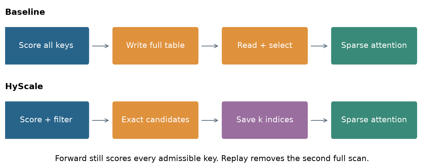
Figure 1. Explanatory diagram based on [1, Figures 2–3]. HyScale still scores all admissible keys in the forward pass. It avoids the full table and later reuses the resulting indices. Arrows show dependencies, not measured durations.

2. Prerequisites: three different kinds of state

Queries, indexer keys and attention latents

The indexer and the attention operator are related but distinct. In the paper’s DSA example, an indexer query has multiple heads, while each context entry supplies a shared indexer key. An inexpensive score aggregates rectified dot products across these heads. The main attention operator uses a separate query and the selected attention KV states. With multi-head latent attention, or MLA, these states are represented using compressed latents and positional components.

Mixing the two key representations obscures the systems argument. Selection needs indexer keys before it can decide what to keep. Attention needs the KV latents after the decision. The two data transfers therefore do not need to finish at the same point. Similarly, the indexer’s gradients and the main attention gradients have separate consumers. This distinction is the basis of the communication-overlap design, not merely a naming convention.

Let $L$ be the context length, $P$ the context-parallel size, and $n=L/P$ the nominal number of local queries. The admissible context of query $t$ contains $L_t$ entries after causal and sequence-boundary restrictions. The paper often writes dense rectangular costs using $L$ as an upper bound. Early queries and block-level selection can have smaller actual candidate universes. A faithful implementation must respect those masks even when it changes how results are stored.

Activations, decisions and checkpoints

Activation recomputation trades computation for memory. A training system saves a layer input, discards internal results, and reruns the layer when backward needs them. This is usually sensible for large continuous tensors. A top-k index set, however, is much smaller than the score table that produced it. Recomputing the table merely to rediscover the same indices can be wasteful.

There are three separate objects: the full table of candidate scores, the selected index set, and numerical quantities evaluated on that set. Saving indices does not magically save every intermediate required by backward. Conversely, needing selected numerical values does not imply needing every rejected value. HyScale’s replay policy exploits this middle ground.

Exactness has a scope

Exact top-k means returning the same selected entries under a defined ordering of scores and ties. It does not mean reproducing dense attention, because the model itself uses sparse attention. Nor does exact support selection by itself establish bitwise reproducibility of a distributed training run. Floating-point accumulation, collectives and other kernels can have their own nondeterminism.

The paper specifically addresses nondeterminism caused by candidate-buffer insertion order and selected-entry ordering. Keeping that scope clear makes its claim stronger: there is an identifiable source of variation, a specific remedy, and a tractable contract. It would be much harder to justify a blanket guarantee for every training component.

3. The mathematical contract that makes replay possible

For admissible entries $u\in\mathcal U_t$, write the DSA indexer score, selection and sparse attention output as

$$\begin{aligned} z_{t,h,u}&=(q^I_{t,h})^\top k^I_u,\\ I_{t,u}&=\sum_{h=1}^{H_I}w_{t,h}\operatorname{ReLU}(z_{t,h,u}),\\ T_t&=\operatorname{TopK}_{u\in\mathcal U_t}(I_{t,u}),\\ o_t&=\operatorname{Attn}\bigl(q_t,\{c_u:u\in T_t\}\bigr). \end{aligned} \tag{1}$$

Here $q^I$ and $k^I$ belong to the indexer, while $q$ and $c$ belong to attention. $H_I$ is the number of indexer heads. The selector chooses entries, not differentiable probabilities. Away from score ties or rank crossings, its output is locally constant. The model’s training rule differentiates through the selected scores, rather than through an infinitesimal motion of the selected indices. [1, Equations 1–4, Appendix A]

Let $p_t$ be the detached target distribution obtained from the sparse attention weights, averaged over heads. The indexer predicts a distribution only over the selected entries:

$$\begin{aligned} \widehat p_{t,u}&=\frac{\exp(I_{t,u})}{\sum_{v\in T_t}\exp(I_{t,v})},\quad u\in T_t,\\ \mathcal L_I&=\lambda\sum_t\sum_{u\in T_t} p_{t,u}\log\frac{p_{t,u}}{\widehat p_{t,u}}. \end{aligned} \tag{2}$$

To derive the score gradient, first treat $p_t$ and $T_t$ as fixed. The term involving $p\log p$ is constant. Expanding the other term gives a weighted negative score plus the log-sum-exp over selected scores. Differentiating the former yields $-\lambda p_{t,u}$; differentiating the latter yields $\lambda\widehat p_{t,u}$ because the target probabilities sum to one. Consequently,

$$g_{t,u}=\frac{\partial\mathcal L_I}{\partial I_{t,u}} =\begin{cases} \lambda(\widehat p_{t,u}-p_{t,u}),&u\in T_t,\\ 0,&u\notin T_t. \end{cases} \tag{3}$$

The zero is not a universal theorem about every learned selector. It follows from this particular loss and differentiation convention. If a different loss normalizes over all context entries, uses a full-context teacher distribution, or differentiates through a soft routing mechanism, rejected scores may matter. Replay must preserve the actual objective, not just the visible top-k output.

For the paper’s objective, define $\delta_{t,h,u}=g_{t,u}w_{t,h}\mathbf 1[z_{t,h,u}>0]$. The chain rule then gives

$$\begin{aligned} \frac{\partial\mathcal L_I}{\partial w_{t,h}} &=\sum_{u\in T_t}g_{t,u}\operatorname{ReLU}(z_{t,h,u}),\\ \frac{\partial\mathcal L_I}{\partial q^I_{t,h}} &=\sum_{u\in T_t}\delta_{t,h,u}k^I_u,\\ \frac{\partial\mathcal L_I}{\partial k^I_u} &=\sum_{t:u\in T_t}\sum_h\delta_{t,h,u}q^I_{t,h}. \end{aligned} \tag{4}$$

Every sum is restricted to selected entries. Backward still needs selected per-head inner products or equivalent information for the rectifier gates; the small scalar score alone does not erase that requirement. In the default index-replay path, the relevant values are regenerated from the saved input and selected indices. Since the indexer’s inputs are detached in this architecture, these gradients train its projection weights without sending the indexer loss back through the main attention pathway.

This derivation explains why selection replay is more than a conventional checkpoint configuration. It changes which entries an operator recomputes. An ordinary policy that saves top-k output but reruns the entire scoring operator cannot exploit Equation (4).

4. The memory–computation trade-off in concrete units

Consider the paper’s one-million-token example: $L=2^{20}$, $n=2^{13}$, $k=2^{11}$, $H_I=32$, and $d_I=128$. If scores are FP32 and indices are 32-bit integers, their persistent storage differs dramatically:

$$\begin{aligned} M_{\rm table}&=4nL=32\ \mathrm{GiB},\\ M_{\rm index}&=4nk=64\ \mathrm{MiB},\\ M_{\rm index+score}&=8nk=128\ \mathrm{MiB},\\ \frac{M_{\rm table}}{M_{\rm index}}&=\frac Lk=512. \end{aligned} \tag{5}$$

These are analytic sizes for one layer on one GPU, not total training memory. They exclude layer inputs, temporary buffers, attention states and other model components. Index replay’s attractive 64 MiB number should therefore not be confused with HyTopK’s measured peak allocation, which includes its candidate buffers. The paper reports 1.5–1.9 GiB for that selection operation. [1, Table 1, Figure 11]

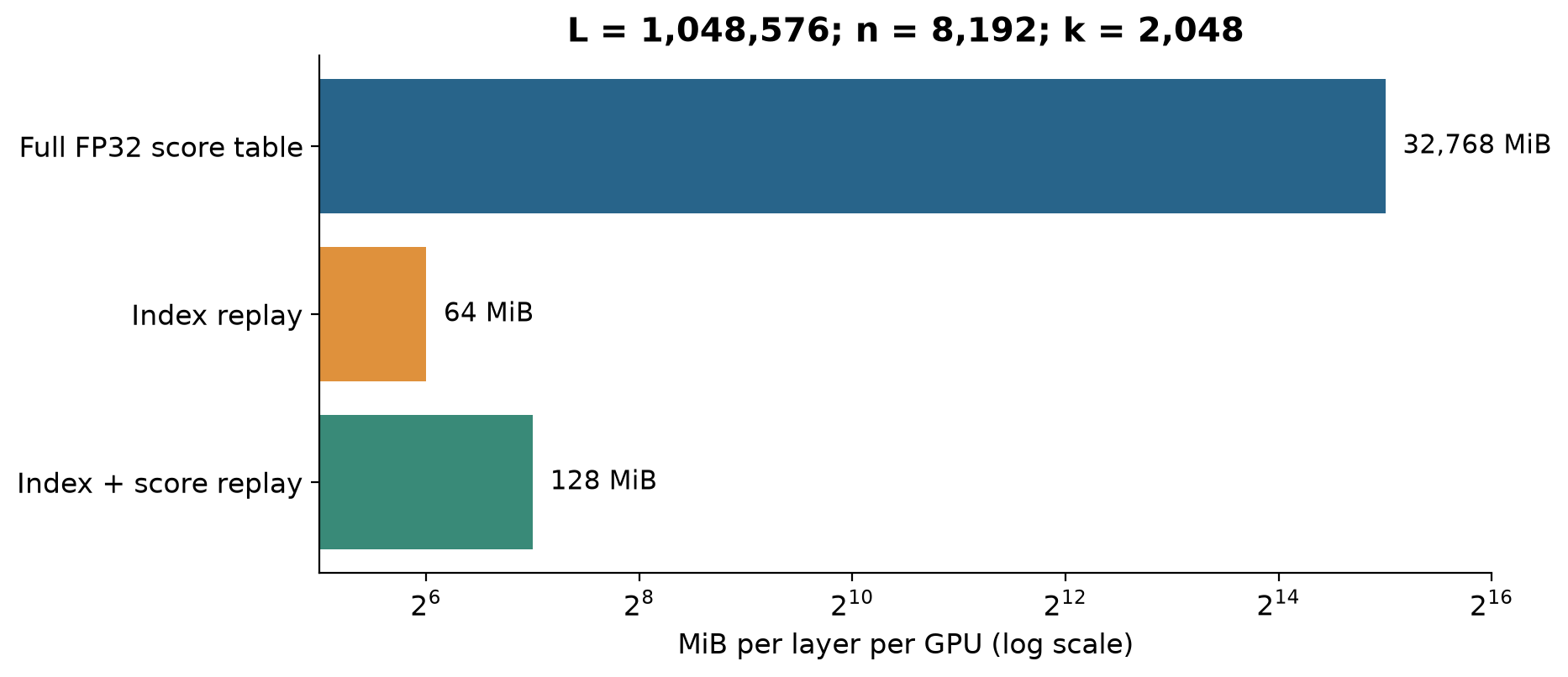
Figure 2. Analytic storage from [1, Table 1], using binary units. The logarithmic axis prevents the two small replay states from disappearing. This is not a chart of whole-model peak memory.

Ignoring small bookkeeping terms, the dominant dot-product recomputation changes from $2nLH_Id_I$ to $2nkH_Id_I$. The factor of two counts a multiply and an add. Under the dimensions above, these counts are approximately 70.37 trillion and 0.1374 trillion operations. Their ratio is 512, but no 512× wall-clock speedup follows: gathers, projections, attention, communication and fixed launch overhead remain.

The operator-level alternatives each retain an unwanted cost. Full recomputation saves no selection state but regenerates the full search. Saving only the indexer inputs avoids some projections but still scores all keys. Saving the full score table avoids the dot products but pays its large memory footprint and still needs selection. Saving top-k indices is useful only if the recomputed scoring operation actually restricts itself to those indices.

HyScale distinguishes index replay from score replay. The former stores indices and regenerates selected scores; the latter additionally retains those scores. The paper prefers index replay because its selected rescoring accounts for at most 1.6% of a training step and saves about 5 GiB per GPU relative to score replay in its GLM-5.1 configuration. That is an empirical configuration-specific argument, not a rule that extra recomputation always wins. [1, Section 3.3]

One further option is to offload indices to pinned host memory. The forward copy overlaps sparse attention; the return copy overlaps projections during recomputation. This is attractive only if the copies finish before their consumers and do not interfere too severely with other transfers. The saved object is compact, but it is still real traffic with a lifetime and ownership that the runtime must track.

5. HyTopK: use an optimistic threshold without approximating the answer

Why sampling is useful

Suppose a query has a million scores but retains only 2,048. Writing every score to device memory is expensive. A fused scorer can instead compare each computed score with a threshold and write only passing candidates. An exact selection over that smaller set completes the operation. The threshold is therefore a device for shrinking an intermediate representation.

A conservative threshold below the true k-th score guarantees that every desired entry survives, but can admit too many candidates. A threshold based on nearby queries’ selections can be particularly weak when their preferences differ. Context parallelism also complicates dependence on neighboring queries, since their decisions may be produced simultaneously on different GPUs. HyTopK samples from each query’s own admissible context instead. [1, Section 3.2]

For a sufficiently long context, the paper chooses the sample count and order statistic as

$$\begin{aligned} M_t&=\min\bigl(\max(4096,L_t/128),8192\bigr),\\ r_t&=\left\lceil\frac{3kM_t}{L_t}\right\rceil,\\ \tau_t&=\text{the }r_t\text{-th largest sampled score}. \end{aligned} \tag{6}$$

The factor three aims to admit roughly $3k$ candidates under a representative sample. This is an expectation-based motivation, not a distribution-free buffer bound. At $L_t=2^{20}$ and $k=2048$, the rule yields $M_t=8192$ and $r_t=48$. The 48-th sampled score estimates a cutoff near the 6,144-th population rank. The default buffer has 16K slots, giving further room for sampling error.

Several adjacent queries can share sampled key positions and score them in one matrix multiplication. That is different from borrowing a neighbor’s selected set: each query still obtains its own scores against sampled context entries. For very short causal prefixes, one cannot sample more distinct admissible keys than exist, and $r_t$ must be a valid sample rank. Equation (6) describes the long-context regime; a complete generalized algorithm needs an exact short-context path or equivalent boundary handling.

Why a bad threshold need not produce a wrong top-k

Let $C_t$ be all entries whose scores pass the threshold. If the scan is complete, no candidate was lost to overflow, and $|C_t|\ge k$, then the top-k entries of the full universe are contained in $C_t$. Every omitted entry lies below the threshold, while at least k included entries meet it. Selecting the exact top-k from $C_t$ therefore gives the exact full result. Ties require a consistent inclusive comparison and secondary ordering.

This is a useful distinction: an optimistic threshold may fail to produce a usable candidate set, yet the overall algorithm can remain exact by detecting that failure. Too few candidates means the threshold was too high. Too many candidates for the buffer means the recorded set cannot be trusted. Both cases trigger rescoring and exact selection for that query.

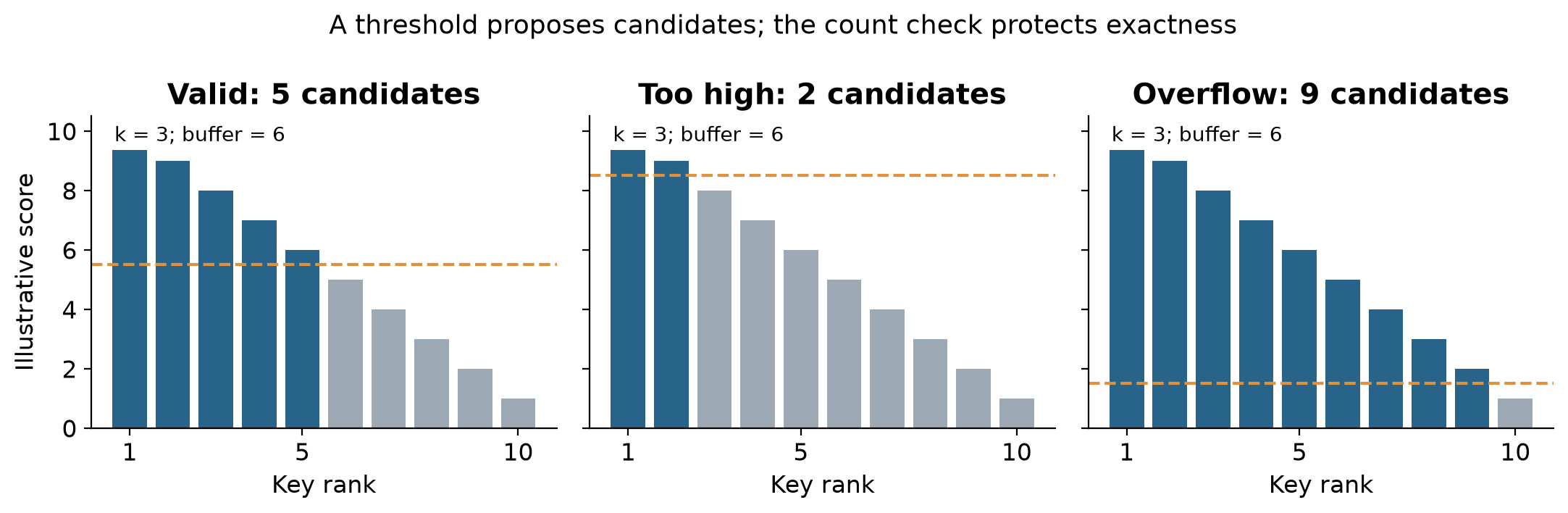
Figure 3. Constructed example, not paper measurements. With k = 3 and a six-entry buffer, the middle and right cases require recovery. In the left case, exact top-k over five candidates recovers the true result.

Algorithm 1. Exact selection with optimistic filtering

The following is explanatory pseudocode. It expresses the correctness conditions and includes a conservative short-context fallback; it is not a transcription of a particular kernel.

1. For each query, form its admissible key universe U.
2. If U is too short for the sampling rule, select exactly.
3. Otherwise score a strided sample and estimate threshold tau.
4. Scan every key in U; append every score >= tau to candidates.
5. Record the true candidate count and any buffer overflow.
6. If count < k or overflow occurred, mark this query failed.
7. For valid queries, select k candidates by (score, position).
8. For failed queries, rescore U and select its exact top-k.
9. Order each final selection by score, breaking ties by position.
10. Save the ordered indices for attention and later replay.

The key invariant is that no query consumes a truncated or undersized candidate set. Host-free recovery checks failures on the GPU, stores their count there, and launches a fixed chain of recovery kernels. These return immediately when no failures exist. Up to 64 failed queries are handled by the targeted path; the paper states that more than 64 triggers a full rescore fallback. In the observed selections, no more than four queries failed. [1, Sections 3.2, 4.6]

The distinction between a cheap common path and a correct rare path matters more than a claim that failures never happen. Correctness comes from complete recovery. Average speed depends on the failure distribution and recovery cost. A workload with many ties, unusual score concentration, or a poorly representative stride can remain correct while losing much of the speed advantage.

6. Determinism and replay are related, but solve different problems

Atomic appends can put the same passing candidates into a buffer in different orders. If the k-th score is tied, that order can change the selected set. Even with the same set, a different order of accumulation can change floating-point results. Sorting every candidate by position would restore order but can be unnecessarily expensive.

HyTopK instead makes ordering decisions only where they affect the answer. Among keys tied at the cutoff, it retains the smallest positions. It then orders the k retained entries by score and position. The paper uses radix selection for cutoff ties and radix sorting for the final set. Candidate insertion may remain nondeterministic internally, while the visible selection contract is deterministic. [1, Section 3.2]

A small example clarifies why both steps matter. Suppose scores are $(9,8,8,8)$ and k is two. Position-based tie handling chooses the earliest of the three eights. Merely sorting whichever two elements an atomic buffer happened to retain would not fix set membership. Conversely, selecting the right two positions but leaving their output order unspecified does not define the later floating-point accumulation order.

Replay then avoids having to make the decision again. With the same layer input and relevant stochastic state, recomputation loads the forward indices and regenerates selected numerical values. It does not ask a possibly different search execution to rediscover the support. This is especially useful around ties: the backward pass follows the support actually used in forward, rather than a newly chosen support that happens to have equal scores.

Algorithm 2. Index replay through a training layer

1. Forward: compute indexer and attention projections.
2. Gather required indexer keys; run exact HyTopK.
3. Save the selected indices, optionally to pinned host memory.
4. Run sparse attention and the selected-entry indexer loss.
5. Discard recomputable activations according to checkpoint policy.
6. Recompute: restore the same layer input and required RNG state.
7. Restore saved indices and recompute the needed projections.
8. Gather and score only the selected entries for each query.
9. Recompute sparse attention on the identical selected support.
10. Backward: accumulate selected-entry gradients and reduce-scatter.

The saved indices must belong to the correct layer, microbatch, sequence layout and forward invocation. Reusing a stale set across optimizer updates would define a different training procedure. Replay is reuse within one forward/backward computation, not cross-step approximation. Likewise, changes in masks, sequence packing or index permutation must be reflected consistently in the saved representation.

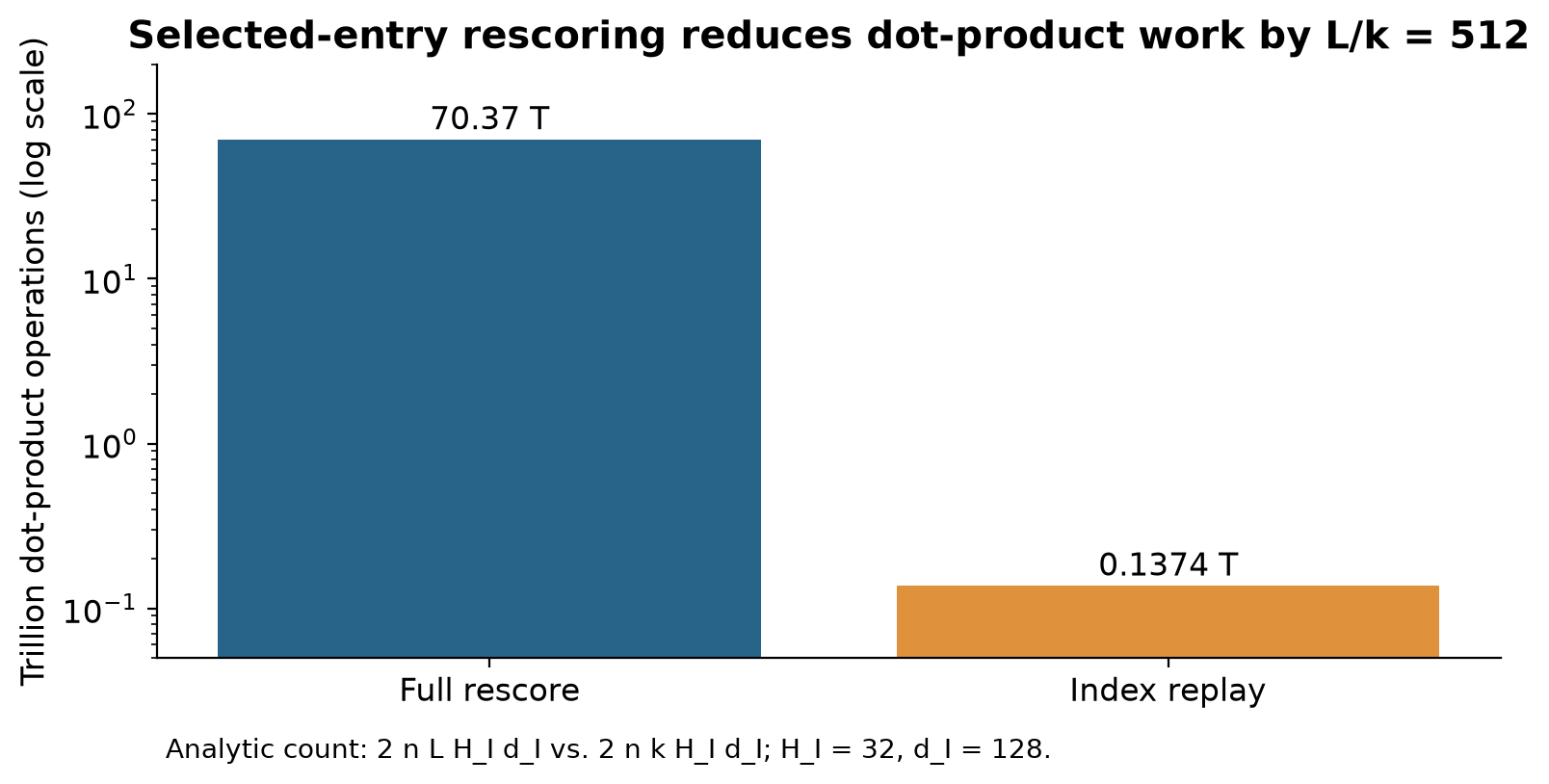
Figure 4. Analytic operation counts using [1, Table 1]. The 512× ratio applies to the indicated dot-product work, not total layer time or total training time.

7. Sparse attention backward needs the same support

Appendix A completes the argument by examining the main attention path. For one head, let $\ell_u=q^\top c_u/\sqrt d$ on the saved support, $a=\operatorname{softmax}(\ell)$, and $o=\sum_u a_uc_u^V$. For an upstream gradient $\bar o$, first differentiate the weighted sum with respect to its weights. The result is $\bar a_u=\bar o^\top c_u^V$. Multiplying by the softmax Jacobian subtracts the attention-weighted average of these values:

$$\begin{aligned} \bar\ell_u &=a_u\left(\bar a_u-\sum_{v\in T}a_v\bar a_v\right)\\ &=a_u\left(\bar o^\top c_u^V-\bar o^\top o\right),\quad u\in T,\\ \bar q&=\frac1{\sqrt d}\sum_{u\in T}\bar\ell_u c_u. \end{aligned} \tag{7}$$

The latent gradient has a key contribution proportional to $\bar\ell_u q/\sqrt d$ and a value contribution proportional to $a_u\bar o$, with the latter applied to the value part of the latent. These contributions accumulate across all queries and heads that selected the entry. No unselected entry is needed for this layer’s sparse-attention backward. The detached target of the indexer loss also avoids an additional gradient path through the main attention probabilities. [1, Appendix A]

Under context parallelism, each rank computes partial key and latent gradients from its local queries. Reduce-scatter sums those contributions and returns each position’s gradient to its owner. Saving the selected support does not remove this collective. It changes the local work leading up to it, which can in turn change what communication is exposed on the critical path.

This distinction also explains why replay is not simply a sparse backward implementation. Sparse backward already restricts its sums. The waste arises earlier, when generic recomputation reconstructs a dense selection process so that sparse backward can begin. HyScale aligns recomputation with the dependency set that backward actually needs.

8. Communication overlap follows consumers

The baseline gathers indexer keys and attention KV states before selection. That creates a stronger synchronization barrier than the dataflow requires. Selection consumes only the indexer keys. Attention needs KV states later, once selection has finished. HyScale separates these transfers and waits for each at its first consumer. Indexer-key communication can overlap query projections, while KV communication can overlap projections and selection. [1, Section 3.4.1]

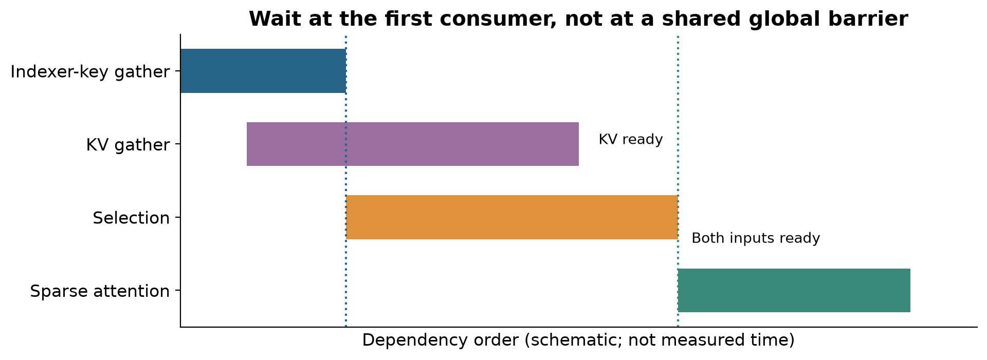
Figure 5. Explanatory dependency schedule based on [1, Figure 3]. Bar lengths are illustrative. The diagram does not claim all communication is hidden in a measured run.

For intuition, suppose projections are complete and ignore resource interference. If selection takes $S$, KV gathering takes $G$, and attention takes $A$, a serialized path takes $S+G+A$. Starting the gather alongside selection gives an idealized path

$$T_{\rm overlap}=\max(S,G)+A, \qquad \Delta T_{\rm ideal}=\min(S,G). \tag{8}$$

This is a dependency bound, not a performance prediction. Communication can compete with kernels for memory bandwidth and execution resources. The indexer-key gather has its own prerequisites. Moreover, reducing selection time can expose KV communication that was previously hidden. An optimization can therefore improve computation while reducing the amount of available overlap.

Backward offers complementary opportunities. The KV-gradient reduce-scatter can run during indexer backward; the indexer-key-gradient reduce-scatter can overlap query-projection backward. The important condition is that the overlapped computation does not consume the unfinished collective result. Adding streams without respecting that condition would either be incorrect or introduce an equivalent wait elsewhere.

The paper also explains why familiar dense-attention strategies do not directly solve this case. Ring-style overlap has little attention computation available per selected subset. Head partitioning does not necessarily reduce transfers when all heads share the same indexer key and MLA latent. The relevant question is the physical representation each partition must receive, not the nominal number of attention heads assigned to it.

9. Locality-aware kernels exchange extra arithmetic for fewer loads

Two adjacent queries often select overlapping keys. Processing them independently loads those keys twice and issues separate gradient atomics. HyScale builds their union once, processes both queries in one thread block, and masks entries that belong only to the other query. Shared gradient contributions can be combined before the global atomic update. [1, Section 3.4.2]

If each set has k entries and their intersection is $\rho k$, then

$$|T_t\cup T_{t+1}|=(2-\rho)k, \qquad \frac{\text{union loads}}{\text{separate loads}} =\frac{2-\rho}{2}=1-\frac\rho2. \tag{9}$$

The paper measures average overlap of 71% over 21 of GLM-5.1’s 78 layers on real documents of 128K and 192K tokens. Substituting that value gives a union of $1.29k$, or 64.5% as many distinct per-pair key loads as two independent lists. The implied 35.5% reduction concerns this idealized load count, not all L2 traffic or kernel time. [1, Section 3.4.2]

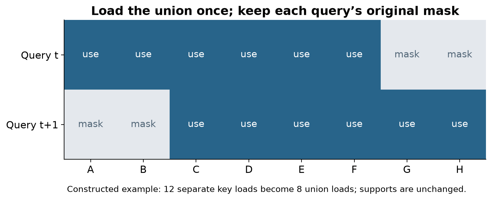
Figure 6. Constructed six-key-per-query example. The first query masks G and H; the second masks A and B. Union processing changes data reuse while retaining each original support.

Why tolerate masked arithmetic? Profiling in the paper shows memory stalls and underused tensor cores in the relevant backward kernels. At 512K on H800, reported L2 throughput is 53–65% of peak, memory stalls occupy 40–44% of warp cycles, and tensor-core activity is only 21–32%. Spending otherwise idle arithmetic capacity can be worthwhile when it saves shared-key loads and atomics.

This is not guaranteed to help every selector. If neighboring queries share few keys, the union approaches $2k$, preprocessing remains, and masked work may dominate. Grouping more than two queries could increase reuse but also enlarge unions, masks and register requirements. The pairwise design is a concrete compromise. Its success depends on the selected-set geometry and hardware bottleneck, not sparsity alone.

10. What the full-model experiment actually measures

The main end-to-end experiment starts from released GLM-5.1 weights and uses 512 H20 GPUs. Each H20 has 96 GB memory; the cluster has eight 400 Gb/s RoCE NICs per eight-GPU node. Global work is fixed at four million tokens per step, with 8K tokens per GPU and one sequence per sample. Both systems use BF16, full activation recomputation, balanced MoE routing and momentum-free SGD with the distributed optimizer. Step times average steps four through ten. [1, Section 4.1, Figure 6]

Those last details matter. A short steady-state timing window demonstrates execution performance under the chosen configuration. It does not demonstrate convergence over a long training run, quality after extensive continued training, or identical behavior under an optimizer with different state costs. Balanced routing also removes one source of irregularity that could matter in other MoE workloads.

Context	Parallel configuration reported	Full-model speedup
256K	PP8 × CP32 × DP2; EP64	1.23×
512K	PP8 × CP64; EP64	1.44×
1M	PP4 × CP128; EP128	2.07×

Expert parallelism is reported as part of the configuration; it should not be naively multiplied with every other axis to infer a larger GPU count. The total remains 512 GPUs. The change in pipeline depth at one million tokens is also part of the experimental setting, so these points are not a pure sweep of sequence length with every parallelism dimension held constant.

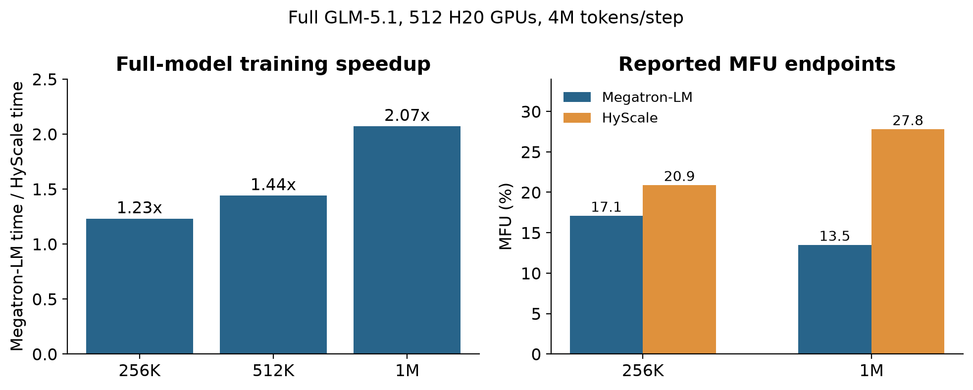
Figure 7. Redrawn from [1, Figure 6 and Section 4.2]. MFU endpoints are reported values; the missing middle MFU value is deliberately not inferred from the plotted curves.

HyScale’s step time grows 1.27× from 256K to 1M, compared with 2.13× for the baseline. Its reported MFU rises from 20.9% to 27.8%, while the baseline falls from 17.1% to 13.5%. Peak GPU memory is similar with replay-index offloading enabled; the paper states that retaining the indices on device would add at most 11%. These are whole-configuration results, not the 512× analytic memory ratio of one temporary table.

At 1M, the profiled first pipeline stage shows forward selection falling from 35.9 to 20.8 seconds and recomputed selection from 37.0 to 1.0 second. Pipeline wait falls from 106.6 to 51.7 seconds. This makes clear why system-level gains cannot be reconstructed by adding isolated kernel speedups: shorter stages change waiting elsewhere in the pipeline. The profiled 264-versus-125-second step shown in Figure 7 is also a separate measurement from the multi-step mean underlying the 2.07× headline.

11. Scaling, ablations and transfer to block selectors

The scaling experiment benchmarks a single GLM-5.1 attention layer on 8–512 H20 GPUs. Strong scaling fixes context length and adds ranks; weak scaling fixes local query count and increases total context. Timings include forward, recomputation and backward on the slowest rank. This makes the experiment useful for diagnosing context parallelism, but narrower than full-model training. [1, Figure 8]

HyScale continues improving as GPU count doubles, although gains fall beyond 256 GPUs because too few local queries remain to hide transfers. The reported doubling gains are 1.65–1.96× up to 256 GPUs and 1.18–1.54× beyond that. The baseline eventually stops improving and can slow down. The paper attributes much of that behavior to rebuilding context-parallel layouts with rank-dependent host synchronization; HyScale caches that layout per microbatch.

The 22.3× comparison at 8M context uses 16K local queries and a single layer. It reflects a baseline that becomes increasingly inefficient as well as improvements in selection. Calling it a universal 22× training acceleration would hide both facts. A useful follow-up would compare against a baseline that already has the layout cache, thereby isolating the remaining selection and communication effects.

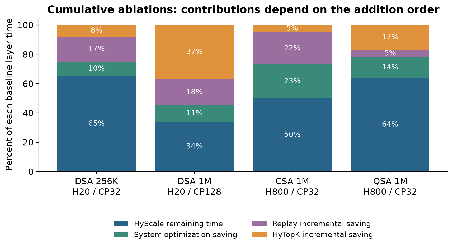
Figure 8. Redrawn from the rounded percentages in [1, Figures 9–10]. Segments show the incremental savings in the reported cumulative sequence: HyTopK, replay, then other system optimizations. Each column uses its own layer baseline.

At 1M on H20, the DSA layer retains 34% of baseline time after all changes. HyTopK accounts for 37 percentage points of savings, replay for another 18, and other optimizations for 11. Together the first two explain roughly 84% of the total 66-point reduction. These are order-dependent incremental contributions. Replay’s marginal gain is measured after the selection path has already been accelerated, so it is smaller than one might expect from comparing an unoptimized full rescan with selected-entry rescoring.

For block-level architectures, the authors instantiate CSA and QSA layers from their papers and evaluate them at 1M on 32 H800 GPUs. The resulting 2.01× and 1.57× layer speedups support transfer beyond token-level DSA. Blocks reduce the selection universe—fourfold in the discussed configurations—so removing dense selection materialization contributes less than in DSA. This is evidence for a common systems principle, with architecture-dependent returns.

12. The rare path deserves as much attention as the fast path

The selection microbenchmark replays captured decisions across all 78 GLM-5.1 layers and context-parallel ranks. With 8K local queries and k = 2048, HyTopK is 1.22–1.71× faster than the baseline’s default memory-limited selection across 256K–1M contexts. Its peak memory stays around 1.5–1.9 GiB. Allowing the baseline a full score table improves its speed but raises peak memory to 12–48 GiB; it remains 3–10% slower in the reported comparison. [1, Figure 11]

The separate recovery experiment injects failed queries deliberately. Sorting alone adds 0.8% relative to base selection. Sorting plus recovery adds 1.8% with one failed query and 4.3% with 64. These are measured overheads under injected failures, not observed probabilities of failure. The observed maximum of four failures per selection belongs to the captured workload, not to a guarantee for every future training distribution.

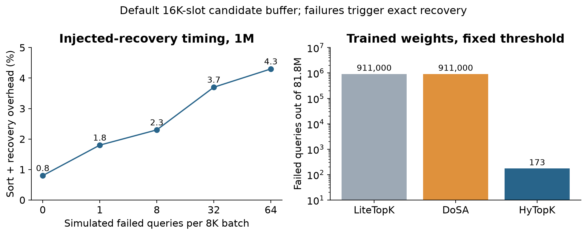
Figure 9. Left: injected-recovery timing from [1, Figure 11b]. Right: failure counts at the default 16K-slot buffer, trained weights and fixed thresholds, from [1, Figure 12a]. The two panels answer different questions.

For the 81.8 million queries captured from one 1M training step, the default-buffer fixed-threshold experiment counts 173 failures for HyTopK versus 911K for each of the two alternative sampling schemes. That is about $2.1\times10^{-6}$ of queries for HyTopK, or approximately 0.00021%, calculated from the reported aggregate count. The number is small, but aggregate averages do not describe clustering by layer, rank or microbatch. Clustering determines whether a fixed 64-query recovery path is sufficient for a particular batch.

With random indexer weights, fixed-threshold HyTopK has zero failures at the default buffer in this experiment. With rising thresholds and trained weights, the reported default-buffer counts are 48 for HyTopK and 483 for each alternative. These distinctions matter: the results do not establish that random initialization, fixed thresholds and trained-weight rising thresholds are interchangeable conditions. They support a specific argument that sampling each query’s own context is more robust than assuming neighboring selections remain representative.

An approximate expectation for runtime helps separate the pieces:

$$\mathbb E[T]\approx T_{\rm scan}+T_{\rm compact} +T_{\rm sort}+\mathbb E[T_{\rm recovery}(F)], \tag{10}$$

where $F$ is the number of failed queries in a selection batch. This expression is explanatory, not a fitted model. Exactness can survive large $F$ through fallback, while expected speed deteriorates. Tail latency and worst-rank completion can deteriorate faster than the mean, especially in synchronized training.

13. Limitations and failure boundaries

The first limitation is objective dependence. The clean replay argument relies on a top-k support treated as fixed during differentiation and an indexer loss defined on that support. A loss that requires all scores invalidates the same storage reduction. A straight-through or differentiable routing estimator needs its own derivation. Reusing the idea requires checking mathematical dependencies, not only finding a top-k call in a model diagram.

Second, the forward search is still dense in its candidate universe. HyTopK removes score-table materialization and improves selection execution; it does not make all indexer dot products disappear. At still larger contexts, the remaining forward scan and global key communication can dominate. Combining replay with methods that reduce the search universe may help, but those methods can introduce approximation or other semantic changes that should be evaluated separately.

Third, the strongest full-model timing evidence covers a short window on one main model and hardware family. The paper does not provide a long-horizon quality trajectory that establishes all convergence behavior under every change. Algebraic equivalence of the intended operations is valuable evidence, but it is not a substitute for characterizing numerical drift, recovery tails and data-dependent locality over prolonged training.

Fourth, locality is measured on a subset of layers and particular document lengths. Learned selectors can change their overlap structure during training or across content types. Highly irregular agent traces, multilingual boundaries or unusual sequence packing could change both locality and sample representativeness. These are plausible stress cases to test, not failures demonstrated by the paper.

Finally, storage and overlap savings have shared resources behind them. Pinned-host offloading competes for transfer capacity; candidate buffers consume real memory; concurrent communication can contend with kernels; cached layouts must remain valid for the actual microbatch. None of these invalidate the design, but they define the conditions under which a clean dependency graph becomes an efficient schedule.

14. Critical analysis: the contribution is a better checkpoint boundary

The most general idea is to checkpoint the sufficient discrete result of an expensive decision. In this layer, the support is the small object that connects forward semantics to backward dependencies. Saving it lets the system discard a large transient search representation while regenerating only the selected numerical values. The boundary between retained state and recomputation moves inside an operator, from whole-tensor policy to entry-level policy.

This perspective also clarifies what is not new by itself. Sparse attention backward already sums over selected entries, and caching indices is an intuitive memory optimization. The stronger contribution is connecting that observation to an exact fused forward selector, a training-compatible recovery procedure, and a distributed schedule. The evidence that these pieces work together is more persuasive than presenting any one of them as a universal solution.

There is an important attribution question in the scaling results. Some gains come from avoiding score-table traffic and repeated scoring; others come from eliminating baseline synchronization or improving kernel locality. These improvements are all useful, but they answer different scientific questions. A reader comparing future systems should distinguish the semantic replay idea from baseline housekeeping improvements. Otherwise, a large speedup against an unoptimized baseline can be mistaken for the intrinsic benefit of sparse selection replay.

I would prioritize three additional measurements. First, show gradient and loss comparisons over a substantially longer training interval, including tied-score cases and varied packed sequence boundaries. Second, report failure-count distributions by layer and rank, including the frequency and time cost of the greater-than-64 fallback under deliberately adverse score distributions. Third, repeat the full-model comparison after giving the baseline the independent layout and boundary caches. These would test numerical behavior, tail robustness and attribution respectively. They are proposed experiments, not results already obtained here.

A fourth question concerns optimization interactions. Faster selection shortens the window that hides KV transfer. Better locality may change bandwidth pressure and the usefulness of overlap. Host offload may consume resources needed by other work. Cumulative ablations establish the quality of one composition, but do not reveal every interaction. A small factorial ablation over replay, overlap and locality would show whether benefits add, substitute for one another, or occasionally interfere.

For a training-system designer, the adoption criterion should therefore be expressed as a contract: the saved support is exactly the one used in forward; recomputation reconstructs all selected numerical dependencies; invalid candidate sets always recover; masks and ownership survive layout transformations; and any performance claim names its workload and scope. HyScale offers a compelling instance of that contract. Its broader value is teaching us to ask which internal decisions deserve to be retained even when ordinary activations are discarded.

15. Conclusion

HyScale shows that learned sparse attention can remain expensive because training systems handle its selection like a large ordinary activation. Its two central mechanisms address different moments in the lifecycle: HyTopK avoids materializing the full score table during the forward scan, and selection replay avoids repeating that scan during recomputation. The selected support remains exact, with explicit recovery when optimistic filtering fails.

The paper’s reported 2.07× full-model speedup at 1M tokens is supported by a coherent account of memory, recomputation and communication. Its larger single-layer scaling gains and block-selector results are useful complementary evidence with narrower scopes. The transferable lesson is to retain the small decision that backward actually depends on, then rebuild only the values needed on that decision’s support.

References

1. Yangshen Deng et al. HyScale: Scaling Long-Context Training for Learned Sparse Attention. arXiv:2610.32057v2, 2026-10-26. Record · PDF. Primary source for the method, all reported measurements and Appendix A derivations.
2. V. A. Korthikanti et al. Reducing Activation Recomputation in Large Transformer Models. 2023. Paper. Background reference cited by HyScale for checkpoint policies.
3. Z. Yin et al. LiteTopK: Exploiting the Curse of Dimensionality for a Fused Indexer-TopK Kernel in Long-Context Sparse Attention. arXiv:2607.11976. Paper. Related sampling approach discussed in HyScale; comparisons here follow HyScale’s experiments.