DFlash: Why a Diffusion Drafter Can Accelerate an Autoregressive Model

Review date: 2026-10-10
Paper: DFlash: Block Diffusion for Flash Speculative Decoding
Paper authors: Jian Chen, Yesheng Liang, Zhijian Liu
Version: arXiv:2602.06036v2, 2026-05-28; first submitted 2026-02-05
Resources: Paper, project, official code
Reading scope: All 13 PDF pages, including Appendix A. Numerical results below refer to v2. New explanatory derivations and illustrative examples are identified separately from the authors’ measurements.

1. The question I think DFlash answers

A speculative decoder can spend surprisingly much time speculating. The large model verifies many positions together, but a small autoregressive drafter still generates its candidates one after another. Making that drafter deeper may improve agreement with the target, yet every extra layer is paid repeatedly along the draft sequence. A method intended to remove a serial bottleneck has inherited a smaller serial bottleneck of its own.

DFlash changes the draft computation. It predicts a block of masked positions in one forward pass, using a small diffusion-style Transformer conditioned on hidden states from the target. The target remains the authority for accepted output. That division of responsibilities lets the drafter make aggressive approximations without turning draft mistakes into unverified final answers.

I find three ideas essential. First, parallel block prediction changes the cost of increasing draft depth. Second, target features enter the key/value inputs of every draft layer, so the small model does not have to reconstruct the whole task from token IDs alone. Third, training mirrors an actual speculative cycle: one clean anchor followed by masked positions, with more loss weight on early predictions.

The result is compelling but conditional. In Table 1, Qwen3-8B reaches 6.08× on MATH-500 at temperature zero with the Transformers backend. Its seven-task average is 4.86×, and MT-Bench is 2.75×. Table 3 reports different experiments on B200/SGLang; there, Qwen3-8B MATH-500 falls from 5.1× at concurrency 1 to 2.8× at concurrency 32. These are complementary observations, not interchangeable performance claims.

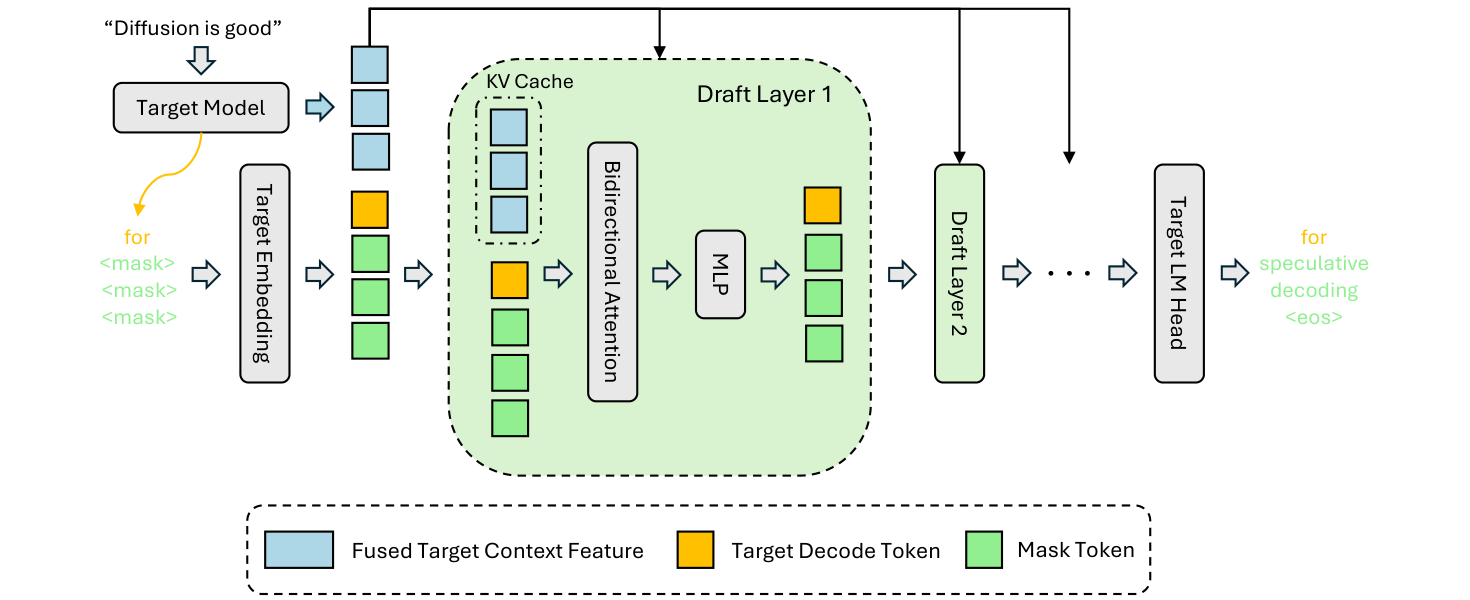
My main takeaway is a design principle: optimize the drafter for useful verified progress per unit time. Standalone language-model accuracy, average token agreement, accepted length, and wall-clock speed are related measurements, but none can substitute for the others.

2. Prerequisites: what is being accelerated?

2.1 Autoregression and the two kinds of parallelism

For a prompt $x$ and continuation $y_{1:T}$, the target distribution factors as

$$p(y_{1:T}\mid x)=\prod_{i=1}^{T}p(y_i\mid x,y_{<i}). \tag{1}$$

This factorization does not stop us from evaluating known candidate tokens in parallel. Given a proposed sequence, a causal Transformer can compute the conditional distribution at each position in one teacher-forced forward pass. What it cannot do in ordinary decoding is know those candidate tokens before sampling them. Speculation supplies the missing guesses.

At small batch sizes, decoding often moves large weight tensors for little arithmetic per step. Evaluating several speculative positions together can use that hardware more effectively. However, verification still has arithmetic, attention, output-projection and cache costs. Once a server is compute-bound, more candidate positions can compete with productive work from other requests. Parallel evaluation is an opportunity, not a promise of zero marginal cost.

2.2 What block diffusion means here

The word diffusion can suggest a long iterative denoising trajectory. DFlash instead uses a single denoising forward pass for drafting. A block starts with a clean token provided by the target; the remaining positions are masks. Bidirectional attention operates among these block inputs, and the drafter predicts the masked tokens together.

This is not equivalent to conditioning position 7 on the actual sampled token at position 6. In a single parallel pass, position 6 was still a mask when the representations were computed. The model can coordinate positional representations, but it does not receive the sampled intermediate continuation as an autoregressive drafter would. That distinction helps explain both the low latency and the limits on long coherent drafts.

For clarity, I use $B$ for the block size, $m=B-1$ for the number of newly proposed tokens, and $\lambda$ for the loss-decay scale. The paper uses $\gamma$ in more than one role. Keeping these quantities separate avoids confusing a speculation budget with a training hyperparameter. A block size of 16 includes the clean anchor; it is not a guarantee of 16 newly accepted draft tokens.

2.3 Accepted length is a prefix statistic

Let $A$ be the number of consecutively accepted draft tokens before the first rejection. Ignoring sequence termination for this derivation, a cycle also produces one target correction or bonus token. The expected output progress is

$$\tau=\mathbb E[A+1] =1+\sum_{k=1}^{m}\Pr(A\geq k). \tag{2}$$

This follows from writing a nonnegative integer as a sum of indicators: $A=\sum_{k=1}^{m}\mathbf1[A\geq k]$. Taking expectations gives the tail-sum expression. The result does not assume independent token errors.

If, only as a teaching approximation, each next token survives with the same conditional probability $a$, then $\Pr(A\geq k)=a^k$ and

$$\tau=1+\sum_{k=1}^{m}a^k =\frac{1-a^{m+1}}{1-a},\qquad a\neq1. \tag{3}$$

For $a=0.8$ and $m=15$, this gives about 4.86 tokens per cycle. For $a=0.9$, it gives about 8.15. These are illustrative calculations, not DFlash measurements. They show why a block of 16 can yield far fewer than 16 tokens and why an early error wastes otherwise plausible later predictions.

3. A latency model that prevents misleading comparisons

3.1 Deriving the break-even condition

Consider many cycles with total draft time $T_d$, verification time $T_v$, and orchestration/cache overhead $T_o$ per typical cycle. If $L_t$ is the baseline autoregressive time per token under the matched workload, the average latency and speedup are approximately

$$L=\frac{T_d+T_v+T_o}{\tau},\qquad S=\frac{\tau L_t}{T_d+T_v+T_o}. \tag{4}$$

The paper’s Equation 1 uses the first two time terms. I expose $T_o$ to make system costs visible; this is an explanatory extension. For variable cycles, the reliable aggregate is total time divided by total emitted tokens, rather than the unweighted average of each cycle’s time-per-token ratio.

Dividing by $L_t$ gives normalized costs $r_d,r_v,r_o$. Acceleration requires

$$S>1\quad\Longleftrightarrow\quad \tau>r_d+r_v+r_o. \tag{5}$$

For example, with $\tau=6$, $r_d=0.25$, $r_v=1.25$, and $r_o=0.10$, speedup is $6/1.60=3.75$. If a larger verification block raises $r_v$ to 2.0 while acceptance stays fixed, speedup falls to about 2.55. Again these are hypothetical costs. Their purpose is to show why a longer accepted prefix does not by itself establish a faster system.

3.2 Why a deeper parallel drafter can win

An autoregressive drafter pays approximately $m\,t_{\mathrm{step}}$ for a linear sequence. DFlash pays one block-forward latency $t_{\mathrm{parallel}}(m,d,L,b)$, which depends on block size, draft depth $d$, context length $L$, and batch size $b$. The dependence on $m$ can be weak over moderate blocks on an underutilized GPU. It is not mathematically constant for all hardware and workloads.

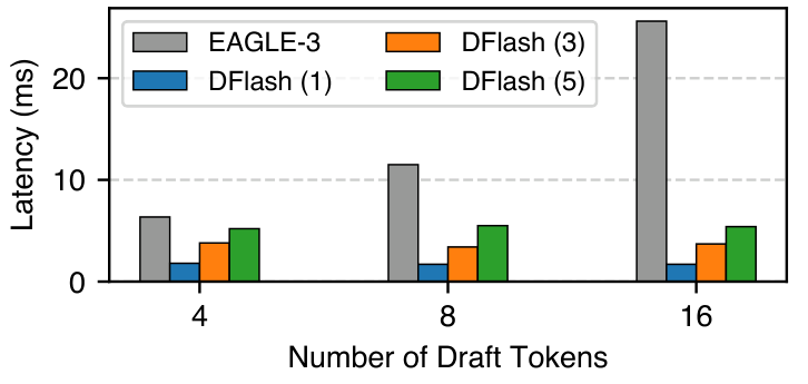
Figure 2 explains the architectural opportunity. A five-layer block drafter may finish before a one-layer autoregressive drafter that repeatedly runs across a longer candidate sequence. That permits spending some recovered latency on depth and better conditioning. The optimum is still finite: Table 6 shows that eight layers raise acceptance but do not consistently improve speed over five layers.

When evaluating a new draft architecture, I would compare a frontier of acceptance versus total cycle cost. Selecting the model with the highest agreement and only later checking its cost reverses the actual objective. Likewise, tree size and block size count different candidate structures; the same number does not guarantee matched verification work.

4. Why imperfect drafts can preserve the target distribution

4.1 Greedy verification is a prefix check

At temperature zero, the target evaluates the proposed sequence with a causal mask. Accept the longest prefix whose tokens agree with target argmax choices. At the first disagreement, emit the target choice and discard the remaining draft suffix. If all candidates agree, obtain a bonus target token. With matched tokenization, logits processing and deterministic tie handling, this recovers the target’s greedy continuation.

It would be wrong to retain correct-looking tokens after an earlier rejection. Their target distributions were computed under a candidate prefix that no longer belongs to the final output. The validity of parallel verification is conditional on the earlier candidates surviving.

4.2 Sampling requires a correction distribution

For nonzero temperature, greedy agreement is insufficient. The following is a derivation of the standard speculative-sampling mechanism cited by DFlash, not an additional algorithm claimed by its authors. At one position, let $q$ be the actual draft proposal law and $p$ the target law given the accepted prefix. Draw $y\sim q$ and accept with probability

$$\alpha(y)=\min\left(1,\frac{p(y)}{q(y)}\right). \tag{6}$$

Define $Z=\sum_z[p(z)-q(z)]_+$. On rejection, sample from the residual distribution

$$r(z)=\frac{[p(z)-q(z)]_+}{Z},\qquad Z=1-\sum_z\min(p(z),q(z)). \tag{7}$$

The accepted probability mass at $z$ is $q(z)\alpha(z)=\min(p(z),q(z))$. Rejection happens with probability $Z$, and residual sampling contributes $Zr(z)=[p(z)-q(z)]_+$. Thus the final mass is exactly

$$\Pr(\mathrm{output}=z) =\min(p(z),q(z))+[p(z)-q(z)]_+ =p(z). \tag{8}$$

If $Z=0$, rejection has zero probability and the residual need not be evaluated. Applying this argument successively to the committed prefix preserves the autoregressive joint law. A parallel drafter need not be an accurate standalone generator for that argument to hold; it must supply the correct proposal probabilities for the actual sampling procedure.

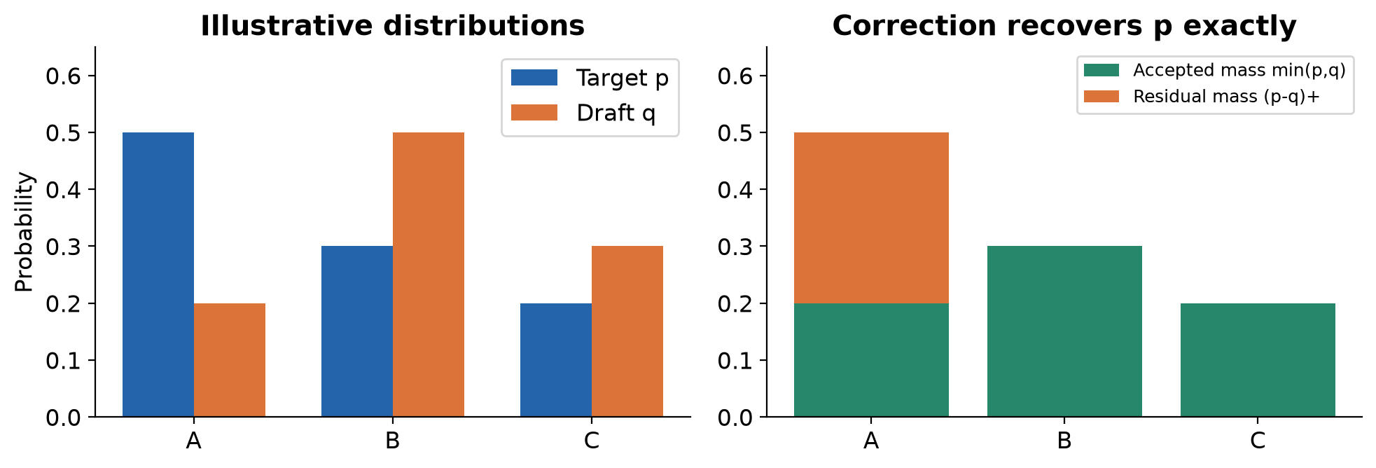
In the example, acceptance totals 0.7. The missing 0.3 mass belongs entirely to token A, so every rejection is corrected to A. Simply resampling from the unmodified target on rejection would generally give the wrong mixture. This small calculation is why I distinguish exact speculative verification from a generic draft-and-refine heuristic.

Algorithm 1. A conceptual exact speculative cycle

Input: committed prefix c, target features, clean anchor a
1. Form [a, MASK, ..., MASK] with block size B.
2. Run the conditioned drafter once; retain proposal laws q_i.
3. Sample the m = B - 1 candidates using those laws.
4. Run the target causally on a and the candidate sequence.
5. Scan positions from left to right under the surviving prefix.
6. At temperature zero, compare with target argmax.
7. For sampling, use min(1, p_i(y_i) / q_i(y_i)).
8. On rejection, emit a target correction (residual if sampling).
9. Discard the rejected suffix; keep only valid cache entries.
10. If all candidates survive, emit a target bonus token.
11. Reuse valid target features; continue from the new anchor.

This pseudocode specifies the mathematical boundary, not repository behavior. Cache bookkeeping must distinguish tokens already committed to output from tokens whose hidden states have actually been computed. The newly sampled correction or bonus token is a clean anchor, but its own target feature may only be computed during the next target pass. Supplying features from a rejected suffix would violate the conditioning assumptions.

5. Target features as persistent draft context

5.1 Fusion before injection

The target first performs prefill and produces the initial token. Hidden states from several selected layers are concatenated and projected to draft width. Appendix A.3 gives the fused representation in the form

$$H_t=\operatorname{RMSNorm}\!\left( W_c[H^{(\ell_1)};\ldots;H^{(\ell_5)}]\right). \tag{9}$$

The five selected features represent different depths of the same target context, not five newly generated continuations. In the main configuration, selected layers range uniformly from the second to the third-to-last target layer. Table 7 compares three with five selected features; five improve acceptance and speed on the three reported tasks.

Fusion happens once before the draft layers. Each draft layer then has its own learned key/value projections. Using the paper’s column-vector convention, the relevant computation is

$$\begin{aligned} Q_i&=W_i^QH_d,\\ K_i&=[W_i^KH_t;W_i^KH_d]_{\mathrm{seq}},\\ V_i&=[W_i^VH_t;W_i^VH_d]_{\mathrm{seq}}. \end{aligned} \tag{10}$$

Target features are memory entries addressed by draft queries. They do not travel through the draft query projection, attention update, output projection or feed-forward network as ordinary draft tokens. This is more precise than saying DFlash simply concatenates target embeddings at the input.

5.2 Why every layer sees the context

Input fusion places target information into the first draft representation and relies on subsequent layers to preserve it. KV injection gives each layer another opportunity to query the target-derived context. The paper motivates this as preventing dilution. I treat dilution as an architectural explanation supported by ablations, not a measured universal law about all deep draft networks.

The design also supports reuse. Context-side key/value entries can be cached across cycles when their underlying committed prefix stays valid. DFlash has a draft-side cache derived from target features; this should not be confused with reusing the target model’s own KV tensors without projection or storage. The two models have different layer computations and cache responsibilities.

5.3 Memory: small projection does not mean zero cache cost

Appendix A.3 uses width 2048, five features and BF16 to estimate projection parameters:

$$5\times2048^2\times2 =41{,}943{,}040\ \mathrm{bytes} \approx42\ \mathrm{MB}. \tag{11}$$

For batch one and sequence length 2048, concatenated inputs take approximately 40 MB and the projected output about 8 MB. These are decimal-MB approximations for that configuration. The paper also reports a temporary projection activation below 400 KB when decoding with block size 16.

These figures describe the fusion component, not the total memory footprint of the drafter and its per-layer caches. If a draft layer stores key/value width $d_{kv}$ for $L$ context tokens, a rough cache estimate across $d$ layers and batch $b$ is $2bdLd_{kv}s$ bytes, with $s$ bytes per stored element. This is my accounting model; head grouping and cache layout change the actual value. Long contexts and many concurrent requests can make a modest per-request addition operationally important.

6. Training the block that inference actually needs

6.1 One clean anchor, then a prediction problem

The training corpus combines roughly 800K prompts from Nemotron Post-Training Dataset V2 and CodeAlpaca, with responses regenerated by the target. Target-generated responses align the training continuation with the model whose tokens must later be accepted. This is a distinct choice from using any high-quality human response: semantically valid alternatives can still disagree with the target and hurt speculative efficiency.

DFlash samples anchor positions from a response. Each sampled anchor becomes the first clean token of a block, followed by $B-1$ masked positions. Unlike fixed segmentation, random starts expose the drafter to many different boundaries, including positions that might follow a rejection during inference.

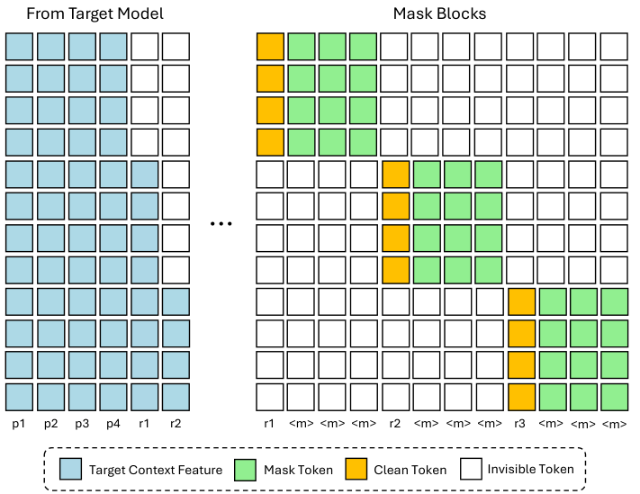
The target can process the clean training sequence once because its own attention is causal. But the draft attention mask must still hide target features containing future response tokens relative to each anchor. A causal target does not automatically make every one of its hidden states legal context for every training block. Blocks must also be isolated from each other: overlapping sampled spans cannot become a back door for clean future-token information.

6.2 Position-weighted cross entropy

Let $y_{a+k}$ be the token $k$ positions after anchor $a$. A compact expression for the training objective is

$$\mathcal L(\theta)= \mathbb E_a\left[ \sum_{k=1}^{B-1} \exp\!\left(-\frac{k-1}{\lambda}\right) \bigl[-\log q_{\theta,k}(y_{a+k}\mid c_a,y_a)\bigr] \right]. \tag{12}$$

Here $c_a$ denotes the legal target-feature context. This combines the paper’s stated cross-entropy training with its position weights in one expression; it is not a claim about a particular reduction or normalization in code. The exponential weight at the first predicted position is one. Later weights decrease, reflecting the fact that a failed early proposal cancels later candidates in a linear speculative prefix.

Equation 2 explains the intuition. Increasing an early conditional survival probability influences many tail probabilities. Increasing only the last survival probability affects the final tail term. Weighted loss is a practical proxy for that asymmetric value, though it is not the exact gradient of latency or expected acceptance. Actual survival probabilities depend on both target and draft distributions, and compute costs do not appear in the loss.

The appendix sets $\lambda=7$ for block size 16, 5 for block size 10, and 4 for block size 8. For $B=16$, the final predicted position has weight $e^{-14/7}=e^{-2}\approx0.135$. That is a substantial preference for the front of the block, not a hard exclusion of the tail.

Algorithm 2. Paper-level training procedure

Input: target-generated prompt/response examples; block size B
1. Keep the target model, shared embedding and LM head frozen.
2. Compute causal target hidden states, online or from a cache.
3. Fuse selected target-layer states into draft context features.
4. Randomly sample legal response anchors for this sequence.
5. Make each training block [clean anchor, B - 1 masks].
6. Allow within-block attention and legal context KV access.
7. Forbid future-context leakage and cross-block attention.
8. Predict masked positions in one draft forward pass.
9. Sum position-weighted cross-entropy losses on predictions.
10. Update trainable draft components; resample anchors later.

Appendix A.1 reports six epochs, AdamW, learning rate $6\times10^{-4}$, gradient clipping 1.0, cosine decay and warmup ratio 0.04. Maximum sequence length is 3072, or 4096 for Qwen3-Coder, with 512 sampled anchors per sequence. The paper also discusses 4K-context base drafters in its separate long-context experiment; I do not silently merge these configurations.

Fixing the number of sampled blocks bounds the amount of masked prediction work. It does not make total training independent of context length: generating or reading target states and attending to longer context still costs resources. Offline feature caching trades target computation for storage and I/O. More selected target layers increase that storage linearly before fusion.

7. Reading the experiments without changing the denominator

7.1 Main instruct-model results

The main Transformers evaluation uses NVIDIA H200 GPUs, thinking disabled and up to 2048 output tokens. EAGLE-3 has two tree budgets, 16 and 60, with seven draft steps and top-k ten. DFlash uses block size 16 for Qwen3, with five draft layers for the small models and eight for Qwen3-Coder in its main recipe.

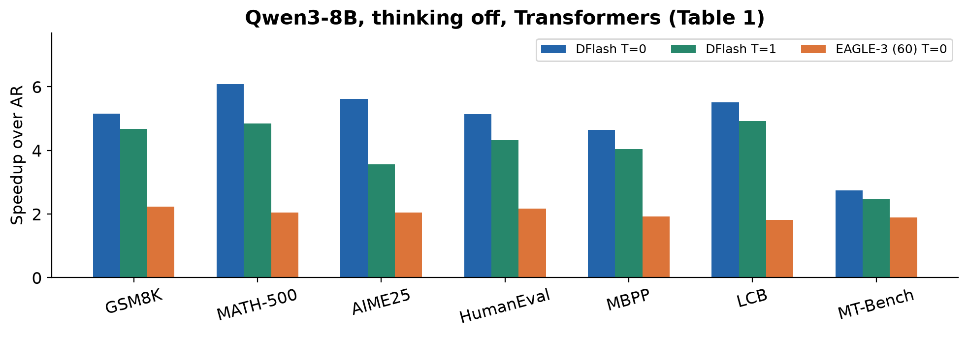
At temperature zero, Qwen3-8B’s DFlash average is 4.86× with $\tau=6.49$, versus EAGLE-3 (60) at 2.02× and $\tau=3.40$. At temperature one, DFlash averages 4.03× with $\tau=5.48$, while EAGLE-3 (60) averages 1.88× with $\tau=3.26$. Sampling makes continuation agreement harder, yet the speed advantage remains in this setup.

I would cite the table values rather than copy the nearby prose’s baseline label. The paper describes an approximately 2.4× improvement while naming EAGLE-3 (16), but dividing 4.86 by 2.02 gives about 2.41, which corresponds to the 60-node row. Dividing by the 16-node row’s 1.76 gives about 2.76. This appears to be a prose/table labeling inconsistency; it does not invalidate the measured rows, but it matters when describing the comparison.

Chat is the clearest counterweight to the headline. MT-Bench reaches 2.75× rather than 6×. Diversity of valid continuations and task-dependent acceptance can matter, although the table alone does not isolate their causal contribution. One should not describe all tasks as sharing the math benchmark’s maximum gain.

7.2 Reasoning is a separate training/evaluation mode

Table 2 evaluates models with thinking enabled, using draft models trained on target responses containing reasoning traces. Qwen3-8B reaches 4.17×, 4.64× and 4.51× on GPQA, MATH-500 and AIME25 at temperature zero. The corresponding temperature-one values are 3.75×, 4.03× and 3.70×.

These results support acceleration of long reasoning continuations in the tested mode. They do not demonstrate that an instruct-only draft checkpoint transfers unchanged to reasoning mode. Nor does faster decoding imply that the target reasons more accurately: the purpose of exact verification is to retain the target behavior while reducing the time required to sample it.

7.3 Serving throughput and concurrency

Table 3 moves to a single B200, SGLang, the stated FA4 attention backend and Spec-v2 scheduling overlap. Those details describe the paper’s experimental environment; they are not an independent recommendation or review of that backend.

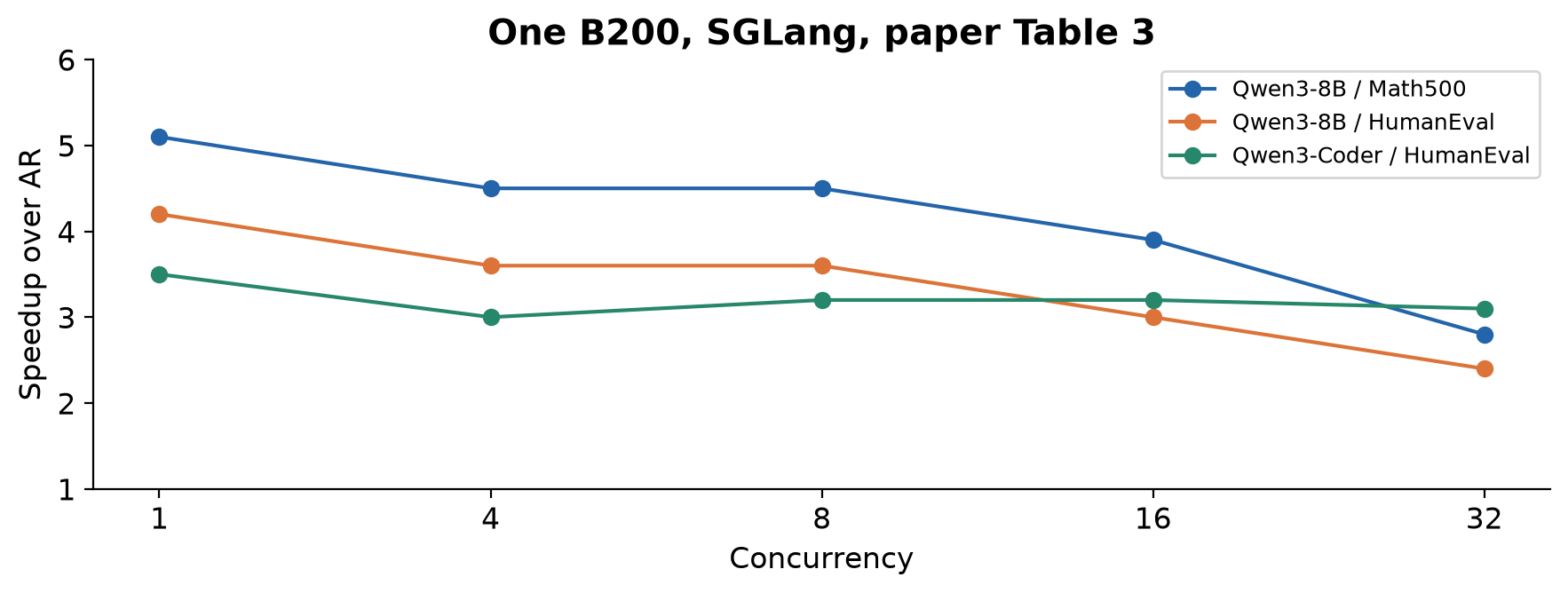
For Qwen3-8B MATH-500, throughput changes from 230 to 1175 tokens/s at concurrency one and from 5694 to 16076 tokens/s at concurrency 32. The latter is still substantial, but it is roughly 2.8×, not 5.1×. Aggregate tokens/s also does not directly specify each request’s time to first token, inter-token latency or tail completion latency.

Table 5 makes an especially useful comparison on LLaMA-3.1-8B with matched UltraChat/ShareGPT training data. It uses SGLang Spec-v1 without scheduling overlap because the paper states Spec-v2 does not support EAGLE-3’s tree drafting. At concurrency 32 on GSM8K, EAGLE-3 (60) falls to 0.6× while DFlash (10) reaches 1.6×. EAGLE-3’s higher average accepted length, 4.55 versus 4.32, does not rescue its speed. This is a concrete demonstration of Equation 4’s denominator.

Appendix A.4 extends to additional models and vLLM. At concurrency eight on SGLang, Qwen3.5-9B DFlash reports 3.5× on Math500 versus native MTP’s 1.7×. For GPT-OSS-120B, gains are 1.6× on Math500 and 1.3× on MT-Bench. These wider results are useful evidence of portability, while also showing that target-model choice changes the achievable gain substantially.

8. What the ablations establish

8.1 Long-context adaptation improves acceptance, not a measured latency guarantee

The authors fine-tune a Qwen3.5-27B drafter on 1.6K LongAlign examples for three epochs. Table 4 measures accepted length at increasing context lengths on LongBench tasks.

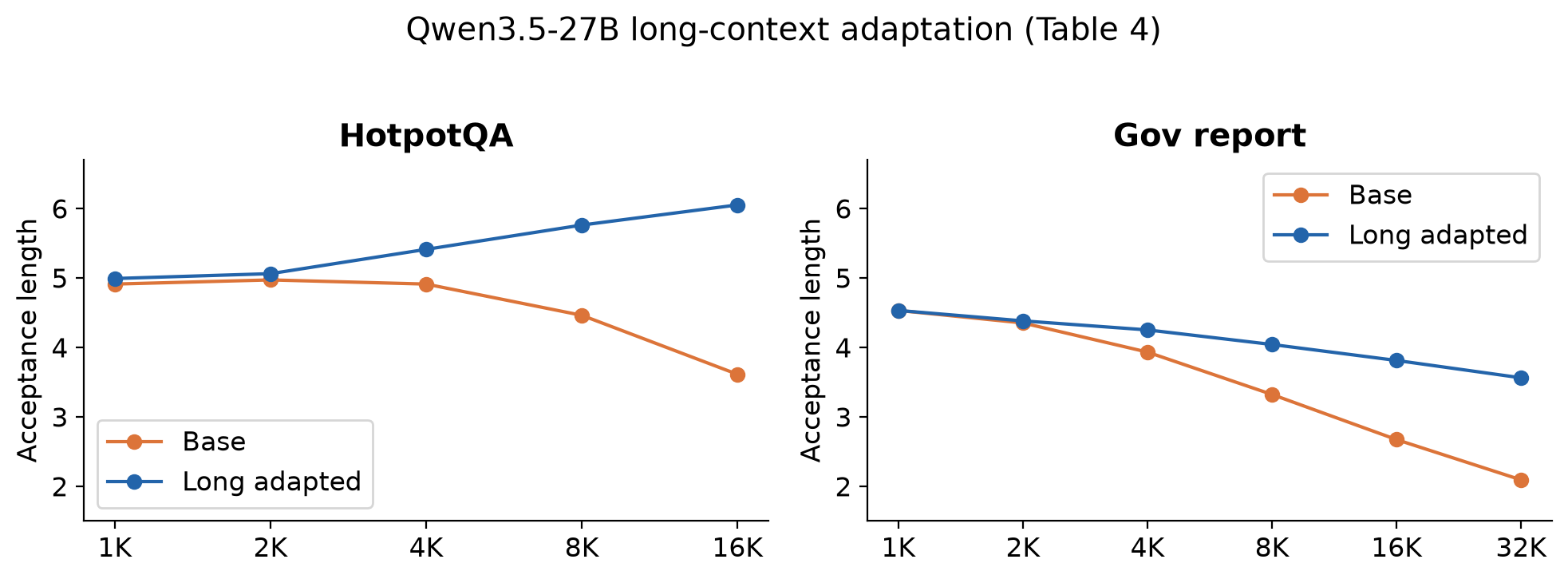
At 16K on hotpotqa, acceptance rises from 3.61 to 6.05 after adaptation. On gov report at 32K, it rises from 2.09 to 3.56. The result shows that a short-context drafter’s declining agreement is not necessarily a fixed limitation of target-feature conditioning. Yet it does not establish how much the longer KV cache costs, or what final speedup remains after that cost. Reporting acceptance as if it were latency would overstate the experiment.

8.2 Depth and selected features

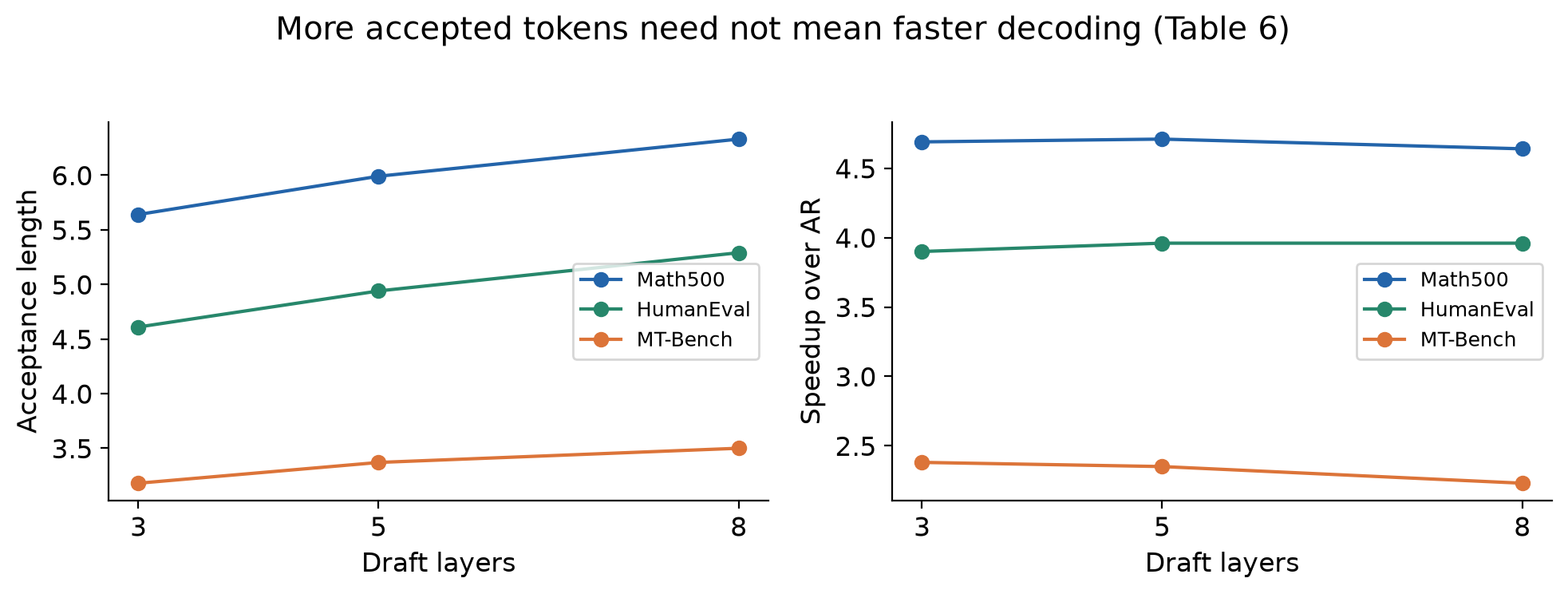
On Math500, moving from three to eight draft layers raises $\tau$ from 5.64 to 6.33, while speed shifts from 4.69× to 4.64×. Five layers reach 4.71×. The small difference between three and five layers should not be oversold without uncertainty estimates. The reliable qualitative conclusion is that greater expressive capacity can help acceptance while additional compute consumes the gain.

Table 7’s three-layer models improve from 4.49× to 4.69× on Math500 when selected target features increase from three layers to five. This supports cross-depth conditioning within the tested configuration. It does not establish that selecting every target layer is optimal, especially when offline storage, feature transport and projection costs matter.

8.3 Conditioning and parallelism are separate contributions

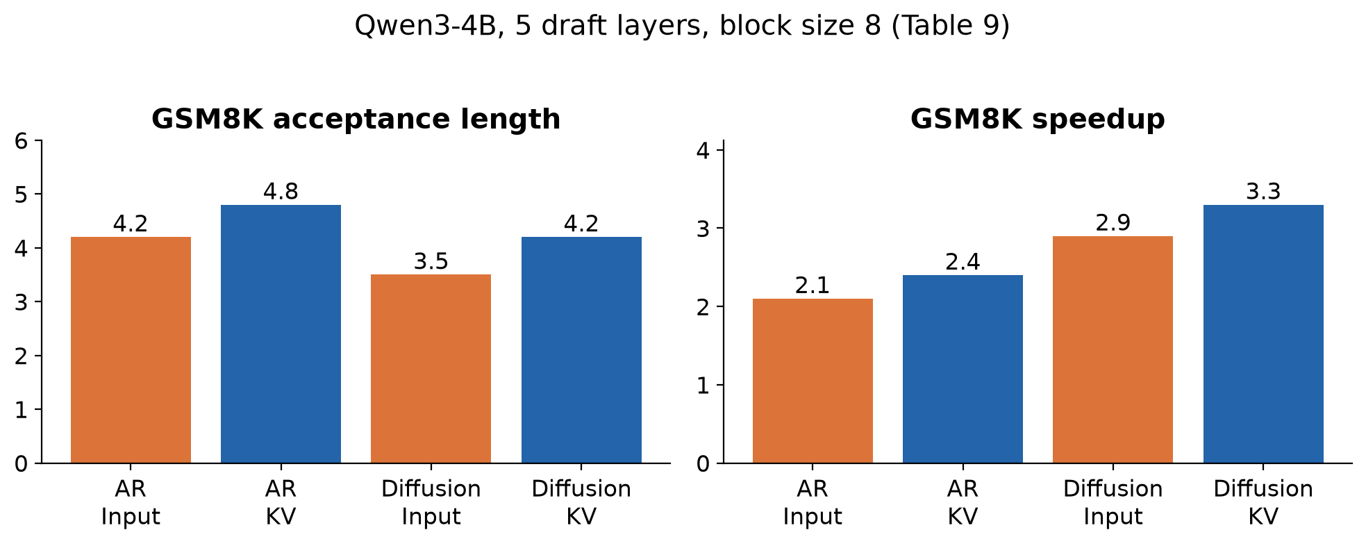
This two-by-two comparison is more informative than a single overall benchmark. Within autoregressive drafting, KV injection improves acceptance from 4.2 to 4.8 and speed from 2.1× to 2.4×. Within block diffusion, it improves acceptance from 3.5 to 4.2 and speed from 2.9× to 3.3×. Both changes help.

Equally revealing, the parallel KV variant has lower accepted length than the autoregressive KV variant, 4.2 versus 4.8, but higher speed, 3.3× versus 2.4×. DFlash’s claim need not be that parallel prediction is always more accurate. Its advantage is the combination of sufficient draft quality and less serial work.

8.4 Block size and random anchors

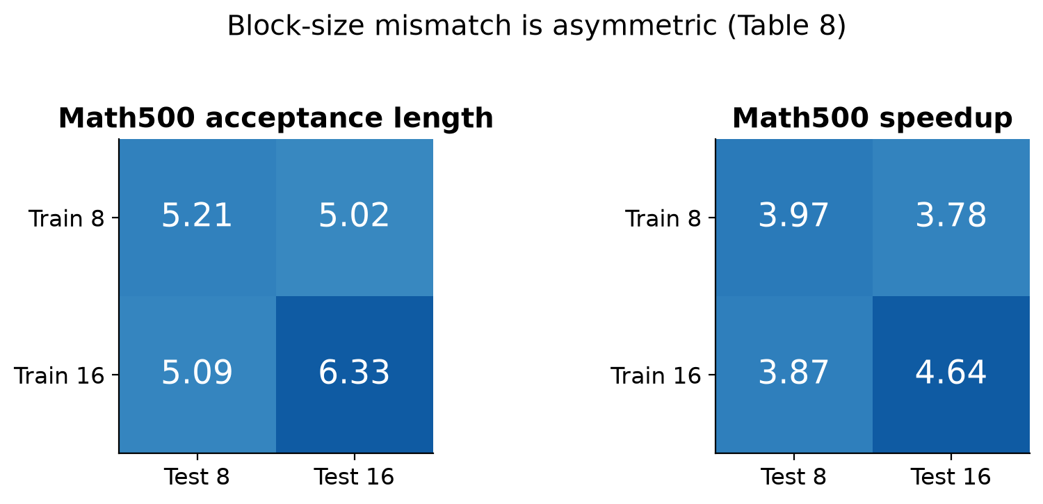
A model trained at 16 and evaluated at eight reaches $\tau=5.09$, close to the 8-to-8 model’s 5.21. Training at eight and evaluating at 16 gives only 5.02, far below the matched 16-to-16 value 6.33. Increasing the inference allocation does not teach the model to exploit a longer horizon. The paper leaves dynamic block-size scheduling for future work; it should not be described as an already demonstrated adaptive controller.

Table 13 compares fixed block construction with random anchors for three-layer models trained on the same 100K subset. On Math500, random sampling raises speed from 4.13× to 4.69× and acceptance from 4.94 to 5.64. On HumanEval, speed rises from 3.29× to 3.90×. This is evidence that matching the training boundary distribution matters in addition to architectural changes.

9. Design alternatives and a practical decision procedure

The natural alternative is a shallow autoregressive drafter. It conditions each position on actual sampled predecessors and may capture dependencies that a one-pass masked block misses. Its weakness is sequential latency. Another alternative is a large pretrained diffusion drafter: more independent capacity, but more resident weights and a larger forward cost. Multi-step denoising can improve draft coherence, yet each step needs to earn back its cost through longer accepted prefixes.

Input fusion is simpler than per-layer KV conditioning but changes the way context persists through depth. Larger blocks expose more parallel work but can waste verification at high concurrency. Multiple draft candidates or trees can recover branching uncertainty, at the price of candidate construction and more verification positions. None of these choices should be settled by acceptance alone.

Algorithm 3. A measurement plan for choosing a draft configuration

Input: target, workload mix, hardware, latency requirements
1. Fix tokenizer, sampling settings and output limits.
2. Measure the matched autoregressive baseline by request class.
3. Sweep a small set of draft depths and inference block sizes.
4. Record total draft, verify, orchestration time and output tokens.
5. Separate prompt processing from steady-state decoding.
6. Measure concurrency, context-length and response-length strata.
7. Track memory occupancy and latency percentiles, not only TPS.
8. Compare complete configurations at the required service level.
9. Keep the fastest feasible option for each measured regime.
10. Re-evaluate after a target-model or workload change.

This is a proposed evaluation plan, not an experiment conducted for this review. It asks whether the method’s advantage survives the actual service objective. A throughput-maximizing configuration can be unsuitable for interactive requests if it worsens tail latency; a low-batch latency win can be valuable even if it disappears near saturation.

10. Limitations and failure boundaries

Target dependence. Hidden-state access and target-generated training data bind a drafter to a target representation and deployment interface. A remote API that exposes only tokens or logits cannot directly supply the same conditioning. A new target revision may change feature behavior even if the output vocabulary remains unchanged.

Parallel proposal coherence. One-pass masked prediction can miss dependencies among sampled future tokens. Increasing block length eventually reaches diminishing returns, especially on diverse continuations. Exact verification protects the final law but cannot recover the time spent producing and checking rejected suffixes.

Workload-dependent cost. Long contexts, large batches, hardware differences and output-head cost can make block drafting or verification expensive. The paper provides useful concurrency and framework results, but those do not cover every service workload, context distribution or memory configuration.

Coverage of comparisons. The main paper states that several diffusion-speculation alternatives were omitted because their implementations were unavailable for that comparison. This limits claims of universal superiority. The matched-data LLaMA ablation strengthens the evidence, but it cannot control every difference across all reported models and backends.

Uncertainty and aggregation. Many tables report point estimates and averages without confidence intervals or detailed latency distributions. Small differences between closely related settings need cautious interpretation. A mean speedup across datasets also does not equal the speedup of a real traffic mix weighted by token counts and request lengths.

Meaning of lossless. Exact verification preserves the target sampling distribution under its mathematical assumptions; it does not prove identical strings for a particular random seed or improve the target’s factual accuracy. Numerical precision, sampling transformations and stopping rules are part of the equivalence boundary. The paper’s headline is an algorithmic property under correct verification, not a blanket claim about every deployment.

11. Critical analysis

11.1 The strongest result is a factorized explanation

I regard Table 9 as the clearest evidence for the mechanism. It separates stronger target conditioning from the removal of serial drafting. The parallel method can win despite a shorter accepted prefix than the autoregressive variant. That directly supports the latency model rather than relying on the visual appeal of a large headline speedup.

The random-anchor ablation contributes a second, less obvious lesson. An inference cycle begins at boundaries created by the verifier, not at neat fixed positions in a training sequence. Sampling anchors approximates that variability cheaply. This is still not full on-policy training on the verifier’s actual boundary distribution, but it addresses a concrete mismatch without requiring sequential rollout at every training step.

11.2 Some explanations are stronger than the evidence

Target features plainly improve the tested drafter, yet describing this as extracting future knowledge should not imply access to future tokens. These are causal representations encoding predictive information. That distinction matters when checking whether the training attention pattern leaks labels and when explaining the method to readers unfamiliar with feature-conditioned speculation.

Likewise, the phrase that parallel drafting cost does not scale with token count is useful only within a hardware regime. A proper claim is that additional positions may exploit spare parallel capacity more efficiently than additional sequential passes. Once attention, matrix multiplication or memory capacity becomes limiting, the apparent flatness can disappear.

The v2 tables are also more informative than the project page’s older numbers. I anchor this review to the versioned PDF and distinguish H200/Transformers from B200/SGLang. Otherwise it is too easy to assemble a fictional best configuration by combining the highest speedup, strongest overlap setting and cheapest memory number from different experiments.

11.3 The next decisive evidence would be end-to-end workload accounting

I would most like to see distributions of accepted-prefix lengths, decomposition of cycle time across concurrency, and matched service-level measurements over realistic mixtures of prompts and response lengths. Those would reveal when the draft model is saving target work and when it is mainly shifting the bottleneck to verification or cache traffic.

A second question is adaptation cost across target changes. The paper’s small long-context fine-tune is encouraging, but accepted length alone does not establish the full operational benefit. Measuring the data-generation, feature-storage and training costs alongside downstream serving savings would turn an attractive inference mechanism into a more complete deployment argument.

My conclusion from the current evidence is positive and bounded: DFlash provides a convincing architecture for converting target representations into cheap parallel proposals. Its most transferable contribution is the joint optimization of conditioning, draft parallelism and verifier-facing training, rather than any one universal speedup number.

12. Conclusion

DFlash works because the draft and target have different jobs. The draft proposes a useful block quickly; the target certifies the output. Persistent KV conditioning supplies rich causal context, one-pass prediction removes repeated draft forwards, and anchor-based weighted training emphasizes the positions that determine usable prefix length.

For my own reading, the essential equations are the prefix tail sum, the complete cycle-latency ratio and the accepted-plus-residual probability identity. Together they explain why the method can be fast, why it can remain exact, and why a larger block or more accurate drafter can still make the system slower. The experiments substantiate substantial acceleration within the tested configurations while leaving workload-aware adaptation and comprehensive service accounting as useful next questions.

References and figure provenance

1. Jian Chen, Yesheng Liang, Zhijian Liu. DFlash: Block Diffusion for Flash Speculative Decoding, v2, 2026-05-28. Main source for method and reported measurements; all 13 pages read.
2. Yaniv Leviathan, Matan Kalman, Yossi Matias. Fast Inference from Transformers via Speculative Decoding. Source of the standard speculative verification framework; Equations 6-8 here are my explanatory derivation of its probability-mass argument.
3. DFlash project and resources. Resource entry point; numerical claims in this review use the versioned paper instead of mixing project-page revisions.

Figures 1, 2 and 4 are cropped from the paper’s Figures 2, 3 and 4, respectively, under its CC BY 4.0 license; the crops remove surrounding prose and retain the visual content. Figure 3 is an original explanatory example. Figures 5-10 are my labeled redraws of Tables 1, 3, 4, 6, 9 and 8. No figure presents newly measured model performance.