SVDQuant: How a Small High-Precision Branch Makes 4-Bit Diffusion Practical

Review date: 2026-10-03
Author: Zhongzhu Zhou
Paper reviewed: SVDQuant: Absorbing Outliers by Low-Rank Components for 4-Bit Diffusion Models
Paper authors: Muyang Li, Yujun Lin, Zhekai Zhang, Tianle Cai, Xiuyu Li, Junxian Guo, Enze Xie, Chenlin Meng, Jun-Yan Zhu, Song Han
Paper ID and version: arXiv:2411.05007v4, 2025-11-08; first version 2024-11-07
Reading scope: Full paper and Appendices A-F. Numerical results below are author-reported unless explicitly identified as my arithmetic or an illustrative example.

1. What I take from this paper

SVDQuant uses a small high-precision computation to make a much larger low-precision computation viable. It protects a low-rank component of a diffusion model’s weights in 16-bit arithmetic and quantizes the remaining component, together with its input, to four bits. Its inference engine, Nunchaku, makes that additional branch affordable by sharing activation reads and output writes with the main branch.

I find the coupling between these two ideas more important than either idea alone. A low-rank approximation can improve a quantized model’s images while simultaneously making the model slower. Conversely, a very fast four-bit kernel is of little use if the denoising trajectory no longer produces a coherent image. The paper explicitly addresses both failure modes: the numerical arrangement of the two branches and their execution on the GPU.

The sequence matters. First, channel scaling moves activation outliers into the weights. Second, singular value decomposition extracts dominant directions from those scaled weights. Third, only the residual weights and the smoothed activations go through four-bit quantization. Finally, kernel fusion keeps the new high-precision branch from repeatedly moving large activation tensors through memory. These operations have different jobs and should not be compressed into the vague claim that SVD removes quantization error.

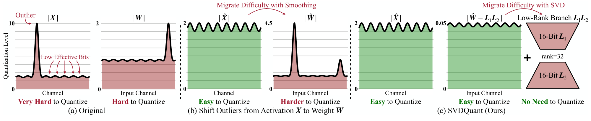
Figure 1 (paper Fig. 3): three numerical stages. Smoothing makes activations easier to quantize but magnifies weight outliers; the protected branch then takes responsibility for the dominant weight directions. The original schematic is reproduced as a crop.

There is also an important distinction from ordinary low-rank compression. SVDQuant does not discard the spectral tail. It retains that tail as a dense, low-bit residual. The full weight transformation is initially an exact decomposition; approximation enters through quantization and finite-precision arithmetic. In an ordinary rank-reduced model, by contrast, the tail itself is deleted. Consequently, the useful rank here can be very small: it buys protection for difficult directions, not a complete representation of the layer.

My reading of the evidence is that SVDQuant offers a strong practical route to four-bit diffusion inference on the tested models and hardware. It does not establish universally lossless generation, a universal speedup independent of workload, or optimality of the final quantized network. The main text, tables, and appendix also contain a few inconsistencies that are worth keeping visible instead of silently averaging away. Sections 9 and 12 explain which numbers I use and why.

2. Prerequisites: bits, matrix products, and denoising

2.1 W4A16 and W4A4 solve different bottlenecks

Let a layer receive $X\in\mathbb{R}^{b\times m}$ and use $W\in\mathbb{R}^{m\times n}$, producing $Y=XW$. Here $b$ is the number of activation rows participating in the product; in an image transformer it can include many spatial tokens even when the image batch size is one. The dense product requires approximately $bmn$ multiply-accumulate operations, or $2bmn$ floating-point operations under the usual counting convention.

W4A16 stores weights using four bits but keeps activations at sixteen bits. A compatible kernel generally expands the weights for higher-precision arithmetic. This can save weight bandwidth and, crucially, allow a model to fit in GPU memory. It does not automatically obtain the throughput of a native four-bit matrix product. W4A4 instead supplies low-bit operands on both sides, so suitable tensor cores can accelerate the dominant multiplication itself.

This distinction is particularly relevant to diffusion transformers: each denoising step processes many image tokens, and the same network runs repeatedly. Weight-only compression may be helpful without directly solving the compute bottleneck. I would therefore qualify the paper’s broad statement that weight-only quantization cannot accelerate diffusion models. Avoiding CPU offload can accelerate an application even when its arithmetic remains high precision. The more precise claim is that weight-only compression does not by itself unlock the W4A4 compute path.

2.2 Quantization grids and outliers

For a group of signed INT4 values, a simple symmetric round-to-nearest quantizer uses the largest magnitude to choose a scale. Ignoring the all-zero special case, its dequantized value is

$$s_Z=\frac{\max |Z|}{7},\qquad Q(Z)=s_Z\operatorname{round}(Z/s_Z). \tag{1}$$

The symmetric grid spans integer codes from $-7$ to $7$. This formulation intentionally leaves aside alternative use of the extra signed code. If a group contains one value of magnitude seven and many values near zero, the step size is one. Many of those small values then share the zero code. A smaller range can preserve distinctions that were previously lost, provided the large component is represented somewhere else.

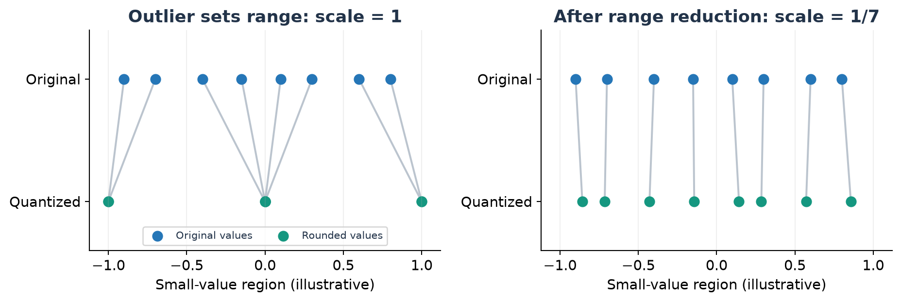
Figure 2 (original illustration): identical small values rounded using scales 1 and 1/7. This is a deliberately simple INT4 example, not an experiment on a diffusion model. The large value setting the left-hand scale is outside the displayed small-value region.

FP4 is not simply INT4 with a different maximum. Its representable values are nonuniform. The paper’s NVFP4 experiments also change scaling granularity: groups of 16 with FP8 scales, versus INT4 groups of 64 with 16-bit scales. Thus an observed NVFP4 advantage can involve both the numerical grid and the finer grouping. Treating it as an isolated proof about floating-point versus integer arithmetic would overstate the experiment.

2.3 Why local errors can change an image

A denoiser is repeatedly called along a trajectory. A useful abstract update is $z_{t-1}=a_tz_t+b_tf_\theta(z_t,t,c)$, where $c$ denotes conditioning. Quantization changes the denoiser’s output and, after the first changed step, also changes later denoiser inputs. A local linearization of the resulting trajectory error gives

$$\delta z_{t-1}\approx(a_tI+b_tJ_t)\delta z_t+b_t\epsilon_t, \qquad J_t=\frac{\partial f_\theta}{\partial z_t}. \tag{2}$$

This is my explanatory model, not a theorem established by SVDQuant. It shows why a small one-layer mean squared error is useful but incomplete evidence. Error may be amplified or damped along the trajectory, and text conditioning can alter which directions matter. It also explains why the paper evaluates both long-step models and their distilled short-step variants instead of assuming one result covers all samplers.

3. Move the difficult values before protecting them

3.1 An exact change of coordinates

Let $D=\operatorname{diag}(\lambda)$ be an invertible diagonal matrix over the input channels. Define a smoothed input and its compensating weight transformation as

$$\widetilde X=XD^{-1},\qquad \widetilde W=DW, \qquad \widetilde X\widetilde W=XD^{-1}DW=XW. \tag{3}$$

Each activation channel is divided by its scale, and the corresponding weight row is multiplied by the same scale. This redistributes numerical difficulty without changing the exact product. Under the row-vector convention $X\in\mathbb{R}^{b\times m}$ and $W\in\mathbb{R}^{m\times n}$, the scale must multiply $W$ on the left. Section 4.2 of the paper prints $W\operatorname{diag}(\lambda)$ in one sentence; that ordering is inconsistent with its stated dimensions. Equation (3) is the dimensionally consistent form used throughout this review.

The appendix uses a SmoothQuant-style family of channel scales,

$$\lambda_i=\frac{\bigl(\max |X_{:,i}|\bigr)^\alpha} {\bigl(\max |W_{i,:}|\bigr)^{1-\alpha}}. \tag{4}$$

These statistics come from calibration data. The migration strength $\alpha$ is searched per layer by examining output MSE after applying SVD. Larger activation-oriented scaling may reduce the dynamic range of $\widetilde X$ while expanding selected rows of $\widetilde W$. Zero or nearly zero channels require numerical safeguards in a practical specification; the conceptual expression assumes nonzero statistics. I do not infer a particular safeguard from the equation alone.

The alternative is to balance outliers between the two operands and stop there. That can work at eight bits, but four bits provide a much smaller representational budget. SVDQuant chooses an asymmetric strategy: concentrate the difficulty on the static weights, where an offline decomposition can find a compact protected component. This is appealing because activations vary with prompt and denoising step, whereas the transformed weight is fixed once calibration is complete.

3.2 What smoothing does not guarantee

The equality in Equation (3) holds before quantization. It does not imply that every choice of $D$ improves the quantized product. Scaling can worsen weight quantization, and calibration maxima can fail to cover a future prompt or timestep. The paper’s method depends on a favorable combination: activations become easier, and the resulting weight difficulty is concentrated in a small number of singular directions.

The phrase “absorbing outliers” is therefore a useful geometric description, not a guarantee that every exceptional entry disappears. A matrix can have many unrelated large entries whose energy is spread across a high-dimensional subspace. In that case a rank-32 branch may leave a substantial tail. This is one reason I would inspect residual distributions across layers rather than treating the paper’s illustrated layer as a universal diagnostic.

4. Derive the error argument before interpreting SVD

4.1 The two operands contribute coupled errors

Write $\Delta_X=X-Q(X)$ and $\Delta_W=W-Q(W)$. Add and subtract $XQ(W)$ inside the product error:

$$\begin{aligned} XW-Q(X)Q(W) &=X\bigl(W-Q(W)\bigr)+(X-Q(X))Q(W)\\ &=X\Delta_W+\Delta_XQ(W). \end{aligned} \tag{5}$$

The triangle inequality separates the terms. Submultiplicativity bounds each matrix product, and $\|Q(W)\|_F\leq\|W\|_F+\|\Delta_W\|_F$ gives

$$\begin{aligned} \|XW-Q(X)Q(W)\|_F &\leq\|X\|_F\|\Delta_W\|_F +\|\Delta_X\|_F\|Q(W)\|_F\\ &\leq\|X\|_F\|\Delta_W\|_F +\|\Delta_X\|_F(\|W\|_F+\|\Delta_W\|_F). \end{aligned} \tag{6}$$

This reproduces the reasoning of paper Proposition 4.1 and Appendix A.1. It makes the coupling clear: activation error is multiplied by a measure of weight magnitude. Protecting a dominant weight component can reduce the matrix through which low-bit activation errors propagate. Merely reducing the storage size of $W$ says nothing about that propagation.

The bound is deliberately conservative. It discards signs, correlations, and cancellation between error terms. It cannot rank all quantization strategies accurately, nor does a smaller upper bound prove a smaller realized error on every input. I use it to motivate a design choice and then look to the experiments for evidence that the choice helps.

4.2 Isolate the quantized residual

Suppose $\widetilde W=L_1L_2+R$, where the factors have shapes $m\times r$ and $r\times n$. The approximate output is

$$\widehat Y=(\widetilde XL_1)L_2+Q(\widetilde X)Q(R). \tag{7}$$

If we temporarily idealize the protected branch as exact, its contribution cancels when subtracting the approximation from the original product:

$$\widetilde X\widetilde W-\widehat Y =\widetilde XR-Q(\widetilde X)Q(R). \tag{8}$$

Equation (6) now applies with $R$ replacing the entire weight. The low-bit activation error multiplies $Q(R)$ instead of $Q(\widetilde W)$. This is the key benefit beyond simply storing a few large weights accurately. The large singular directions are evaluated using the unquantized, smoothed activation on the protected branch, so they are not exposed to the four-bit activation approximation.

The cancellation is algebraic, not a claim of exact sixteen-bit execution. Rounded factors, accumulation, and the final addition introduce further error. A complete implementation-level numerical analysis would retain a protected-branch term $\epsilon_{\mathrm{hp}}$. Here the paper’s simplification is useful for explaining why the dominant error sources become smaller, but it should not be read as a zero-error guarantee for the whole layer.

4.3 Why a smaller residual helps, and where the proof stops

For unclipped uniform nearest rounding, each scalar error is at most half a quantization step. If a single group contains $N$ values, then

$$\|R-Q(R)\|_F \leq\frac{\sqrt N}{2q_{\max}}\max|R|. \tag{9}$$

This follows by squaring the scalar bound, summing over $N$ elements, and taking a square root. If $\mathbb E\max|R|\leq c\,\mathbb E\|R\|_F$, taking expectations yields an upper bound proportional to residual Frobenius norm. The paper uses a looser coefficient without the factor of one half. For grouped quantization, the argument applies separately to each group, and squared group bounds can then be summed.

The distributional condition is where interpretation matters. Truncated SVD minimizes the Frobenius residual, but it need not minimize the maximum entry in every group or preserve the same constant $c$ across candidate decompositions. It also does not directly minimize activation-weighted output error. Thus the proof motivates reducing residual energy; it does not prove that the resulting quantized output is globally optimal.

There is a small mathematical caveat in the appendix’s Gaussian illustration. Bounding the maximum absolute value of $N$ centered Gaussian variables by a generic maximum inequality naturally introduces $2N$ signed variables. A safe standard estimate uses $\sigma\sqrt{2\log(2N)}$, whereas the printed argument uses $\sigma\sqrt{2\log N}$. The latter cannot hold for $N=1$. With a common zero-mean Gaussian marginal, combining the safe estimate with $\mathbb E\|R\|_F\geq\sigma\sqrt{2N/\pi}$ gives the sufficient constant $\sqrt{\pi\log(2N)/N}$. This correction leaves the design intuition intact, but makes the assumptions and constant explicit.

5. What SVD protects, and what refinement changes

For $\widetilde W=U\Sigma V^\top$, order singular values from largest to smallest. The rank-$r$ truncation and its residual satisfy

$$\begin{aligned} L_1&=U_{:,1:r}\Sigma_{1:r,1:r},&L_2&=V_{:,1:r}^{\top},\\ R&=\widetilde W-L_1L_2,&\|R\|_F^2&=\sum_{i>r}\sigma_i^2. \end{aligned} \tag{10}$$

Orthogonality makes the rank-one singular components orthogonal in the Frobenius inner product. Removing the first $r$ therefore leaves exactly the squared energy in the tail. Among all rank-at-most-$r$ matrices, truncated SVD minimizes this residual norm. The optimality concerns an unweighted matrix approximation, not the output distribution of a multi-step generator.

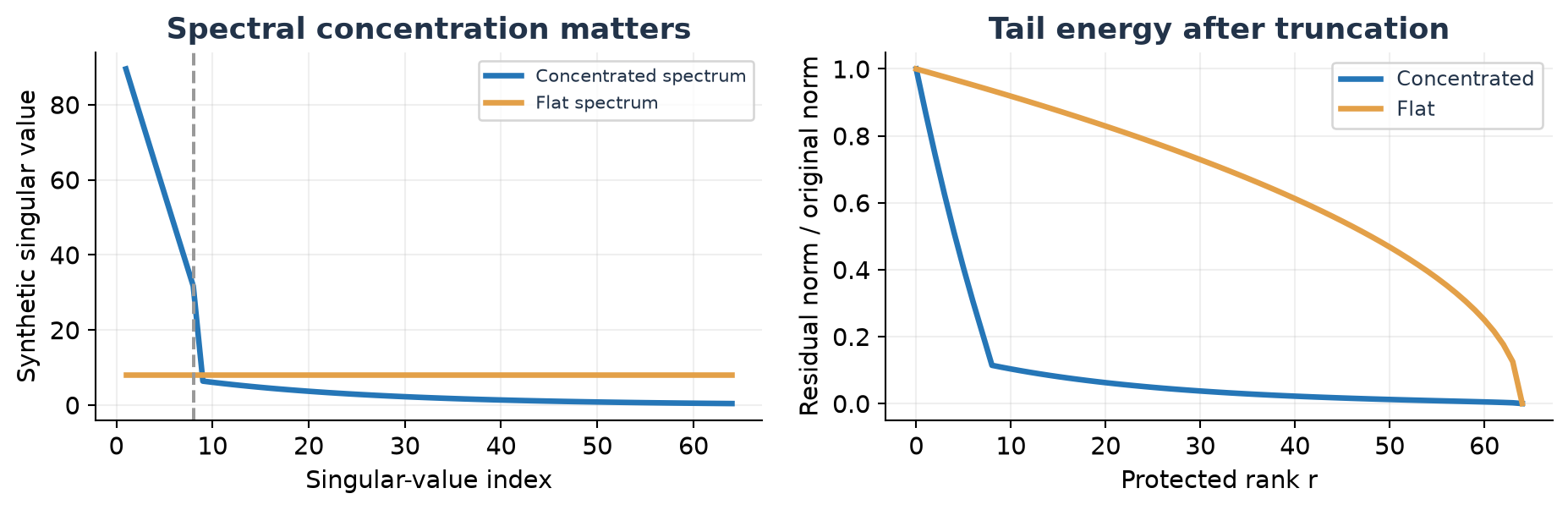
Figure 3 (original analytical illustration): a concentrated spectrum can be protected by a small rank; a flat spectrum cannot. The right panel computes normalized tail energy from the synthetic spectra on the left. No plotted spectrum was measured from a model.

This also explains why order matters relative to low-rank compensation after quantization. If rounding error is spread over many directions, a small correction branch cannot recover much of it. SVDQuant first extracts the structured high-energy component from the transformed weight, then quantizes the remaining matrix. In the paper’s ablation, this arrangement is more effective than simply applying a low-rank correction to an already quantized weight.

The initial SVD is not the whole calibration procedure. Section 4.2 describes alternating updates that decompose the difference between the target weight and the quantized residual, adjust the residual, and retain the smallest-error candidate. In consistent smoothed coordinates, this means using $\widetilde W-Q(R)$ as the candidate protected component. The appendix additionally uses GPTQ for residual weight quantization. Calling the final method “SVD plus nearest rounding” would omit an important part of the evaluated system.

Algorithm 1. Construct and select a protected layer

This is a conceptual transcription of the paper’s described procedure; the candidate set and refinement count are deliberately left as calibration choices rather than invented defaults.

1. Collect representative layer inputs across calibration trajectories.
2. For each candidate migration strength alpha, form D, X/D, and D*W.
3. Compute a rank-r truncated SVD of the transformed weight.
4. Set the residual to transformed weight minus the protected product.
5. Quantize the residual with the chosen group format and calibration.
6. Optionally update the factors from transformed weight - Q(residual).
7. Recompute the residual; retain the best evaluated candidate so far.
8. Select alpha and factors using calibrated layer-output error.
9. Store protected factors, quantized residual, scales, and transforms.

Alternating updates can reduce observed error without guaranteeing a global optimum. Quantization is discontinuous: changing a factor can move a residual entry across a rounding boundary. An iteration that improves an intermediate matrix objective can worsen actual output MSE, so retaining a measured best candidate is sensible. A clear experimental report should distinguish the objective used to select smoothing from the objective used to choose refinement iterates.

I would also keep the distinction between calibration and training. The method uses observed activations to choose transforms and quantize residual weights. That is not data-free compression. It avoids full quantization-aware model training, but calibration data still determine which activation distribution the approximation is designed to preserve. Prompt diversity, step coverage, and guidance settings are therefore part of the method’s applicability, not incidental preprocessing.

6. Nunchaku: a small matrix product can still be expensive

6.1 Count arithmetic and memory separately

The protected branch computes $Z=\widetilde XL_1$ and then $ZL_2$. Its arithmetic relative to the dense product is

$$\rho_{\mathrm{MAC}}=\frac{bmr+brn}{bmn} =\frac r m+\frac r n. \tag{11}$$

For a square $4096\times4096$ weight at rank 32, the ratio is 1.5625%. This is my arithmetic example, not a measured layer from the paper. It is tempting to conclude that the branch must cost about 1.6% extra time. That conclusion is wrong because the two small matrix products may be bandwidth-limited rather than compute-limited.

The down projection still reads a large $b\times m$ input. The up projection still produces a large $b\times n$ output. Reducing $r$ does not reduce those two dimensions. Separate kernels can read the input twice, write separate outputs, and require an additional sum. The paper reports a particularly visible example for QKV projection when the enlarged output exceeds the available cache. Launch overhead and unfavourable small-matrix utilization add further costs.

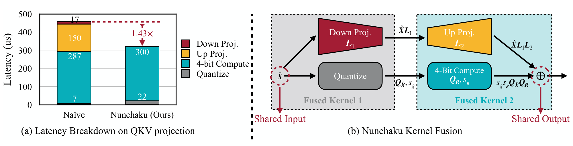
Figure 4 (paper Fig. 6): the down projection shares its input with activation quantization, and the up projection shares its output with the four-bit product. The figure’s 57% overhead refers to its illustrated projection experiment, not every layer or the entire generator.

Nunchaku pairs operations by the large tensor they share. The first fused kernel loads the high-precision activation once, produces its low-bit representation, and computes the down projection. The second combines the four-bit main product and the high-precision up projection before writing the output. The small intermediate $Z$ still exists; fusion does not mean every tensor or every memory access vanishes.

Algorithm 2. Fused execution of a quantized layer

The following describes the dataflow in paper Section 4.3, without assuming a particular thread layout or hardware instruction schedule.

1. Load a tile of the smoothed high-precision activation.
2. Reuse that tile to calculate the protected down projection Z.
3. Quantize the same tile and emit low-bit activation codes/scales.
4. Load the low-bit residual weights and the required activation tiles.
5. Accumulate the low-bit main product with the relevant scales.
6. Compute the protected up projection from Z and the second factor.
7. Combine both contributions before storing the output tile.
8. Apply the ordinary layer epilogue required by the surrounding model.

The fusion benefit is architectural, but not automatically portable. Register pressure, shared-memory use, tensor-core tile shapes, and the rank of additional adapters can change how much useful work fits in a kernel. The paper’s reported 5-10% local overhead should be understood within the tested arrangements. In particular, very high rank can break the premise that the protected computation fits comfortably beside the main operation.

6.2 Storage accounting

For a dense four-bit residual plus sixteen-bit factors, ignoring scales, alignment, bias, and other model tensors, the weight storage ratio is

$$\rho_{\mathrm{bytes}}= \frac{mn/2+2r(m+n)}{2mn} =\frac14+\frac r m+\frac r n. \tag{12}$$

The same $4096$-wide, rank-32 example uses 26.5625% of dense BF16 weight bytes, giving about 3.76-fold ideal compression. Actual model compression is smaller once metadata and retained high-precision components are counted. The paper reports a transformer size reduction from 22.2 GiB to 6.1 GiB, including approximately 0.3 GiB for the low-rank branch. That is about 3.64-fold by direct division.

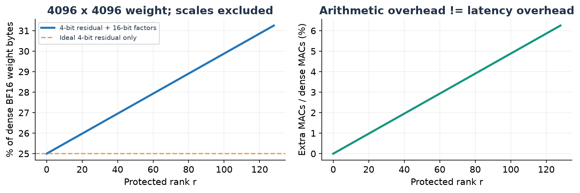
Figure 5 (original accounting): byte and MAC costs for a square 4096-wide layer as protected rank increases. The plots omit scales and all other model components. They do not predict GPU latency.

One should also separate stored model size from peak inference memory. Activations, workspaces, text encoders, the VAE decoder, and memory allocator behaviour can all affect the latter. A device fitting a 6.1 GiB transformer is not necessarily able to execute every requested resolution or batch size within 6.1 GiB. The paper’s roughly 3.5-fold inference-memory reduction and 3.6-fold transformer-size reduction answer related but distinct questions.

7. Why LoRA can remain separate

Suppose an adapter adds $AB$ to $W$, with $A\in\mathbb R^{m\times k}$ and $B\in\mathbb R^{k\times n}$. Applying the same smoothing coordinates gives $D(W+AB)=DW+(DA)B$. Therefore the adapted approximation can be expressed as

$$Y_{\mathrm{adapt}}\approx Q(\widetilde X)Q(R) +\widetilde X \begin{bmatrix}L_1&DA\end{bmatrix} \begin{bmatrix}L_2\\B\end{bmatrix}. \tag{13}$$

An adapter scale can be absorbed into either factor. This derivation explains why the already quantized residual need not be recomputed merely to attach an additive adapter: its contribution can join the high-precision branch. It also makes clear that the adapter factors must be represented in the correct coordinates. Adding an untransformed $A$ to the smoothed layer would implement a different function.

The concatenated representation has at most rank $r+k$. It may have lower mathematical rank if factors overlap, but automatically truncating it back to $r$ would introduce another approximation. Multiple adapters similarly add cost. “No re-quantization” thus describes modularity, not unlimited zero-cost personalization.

The paper shows examples using five community LoRA styles and further examples in Appendix E.2. Those images support the feasibility of integrating existing adapters with the quantized model. They do not establish uniform quality across every adapter, arbitrary adapter strength, or combinations that shift activation distributions far from calibration. The protected adapter product avoids directly quantizing the update, while the rest of the network still contains approximate low-bit computations.

8. Read the experimental setup as part of the claim

The evaluation covers several distinct generator families: FLUX.1-dev with 50 steps, FLUX.1-schnell with four steps, PixArt-Sigma with 20 steps, SANA-1.6B with 20 steps, SDXL with 30 steps, and SDXL-Turbo with four steps. This is a useful range of architectures and trajectory lengths. It gives more confidence than an evaluation on one large transformer, although it remains evidence for the tested image-generation settings rather than all diffusion workloads.

The paper calibrates with COCO captions and evaluates on two separate prompt sets: 5,000 sampled prompts from MJHQ-30K and 5,000 from summarized DCI. The latter condenses long human captions to 77 tokens. That provides a distribution shift from calibration, but does not test preservation of the original thousand-word conditioning. Dataset preprocessing matters when assessing claims about complex prompt alignment.

The quantization settings are also mixed in important ways. Appendix D specifies rank 16 with dynamic per-token activation and per-channel weight quantization for the eight-bit setting. The four-bit setting uses rank 32 and group quantization on both operands. INT4 uses group size 64 with sixteen-bit scales; NVFP4 uses group size 16 with FP8 scales. Residual weights use GPTQ. Inputs of FLUX adaptive-normalization linear layers remain sixteen-bit, giving W4A16 there. For other models, cross-attention key/value projections remain sixteen-bit because they account for less than 5% of runtime according to the paper.

These exceptions are reasonable engineering choices. They also mean that “W4A4 model” is shorthand for the dominant quantized path, not a declaration that every multiplication, tensor, and auxiliary component has four-bit precision. A fair comparison should document the exceptions on both sides.

The metrics answer different questions. FID compares generated and reference image distributions; lower is better. ImageReward is a learned preference proxy; higher is better, but it is not a human study. LPIPS measures perceptual distance to the paired high-precision output, and PSNR measures numerical similarity. A quantized image can have a favorable distributional score while differing from its high-precision counterpart. Conversely, a high PSNR does not establish correct text rendering, object counting, or spatial relations.

9. What the numerical results actually support

9.1 FLUX quality: strong compression, not universal improvement

Table 1 reports the following MJHQ results for FLUX.1-dev. These are copied as numerical data, not remeasured results.

Method	FID down	ImageReward up	LPIPS down	PSNR up
BF16	20.3	0.953	-	-
NF4 W4A16	20.6	0.910	0.272	19.5
SVDQuant INT4	19.9	0.935	0.223	21.0
SVDQuant NVFP4	20.4	0.937	0.208	21.4

Compared with NF4, INT4 SVDQuant improves both preference proxy and similarity here despite also quantizing activations. LPIPS falls by about 18.0%, calculated as $(0.272-0.223)/0.272$. NVFP4 improves similarity further, although its FID is slightly worse than INT4. That is a concrete example of metrics disagreeing rather than a reason to pick whichever metric makes a preferred method look best.

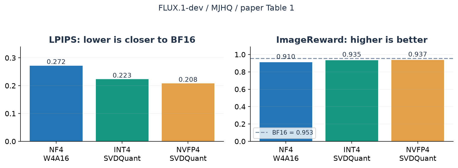
Figure 6 (redrawn from paper Table 1): FLUX.1-dev on MJHQ. The dashed BF16 ImageReward reference makes the remaining gap visible. SVDQuant improves the shown NF4 baseline while remaining below BF16 on this particular preference metric.

Section 5.2 says that the dev variant exceeds BF16 on ImageReward. The displayed Table 1 does not support that wording: 0.935 and 0.937 are below 0.953 on MJHQ; 1.01 is below 1.02 on sDCI. I use the table values and do not repeat the stronger claim. For schnell, INT4 LPIPS on MJHQ is 0.258 versus NF4’s 0.257, another small exception to the prose claim of superiority on every metric. These differences do not negate the method; they narrow the statement the evidence justifies.

9.2 PixArt exposes the role of the protected branch

The smaller PixArt-Sigma model is especially informative. In Table 1, its MJHQ FP16 ImageReward is 0.944. SVDQuant INT4 reaches 0.878, while NVFP4 reaches 0.940. The corresponding LPIPS values are 0.323 and 0.271. This is strong performance relative to the reported low-bit baselines, but INT4 still has a visible quantitative gap to FP16.

Table 3 isolates the low-rank branch and GPTQ. For PixArt-Sigma INT4, neither component gives ImageReward -1.226 and LPIPS 0.762. GPTQ alone gives -0.902 and 0.763. The low-rank branch alone gives 0.858 and 0.356; combining both yields 0.878 and 0.323. In this setting, protecting the low-rank component is the main intervention preventing collapse, while GPTQ improves the already viable approximation.

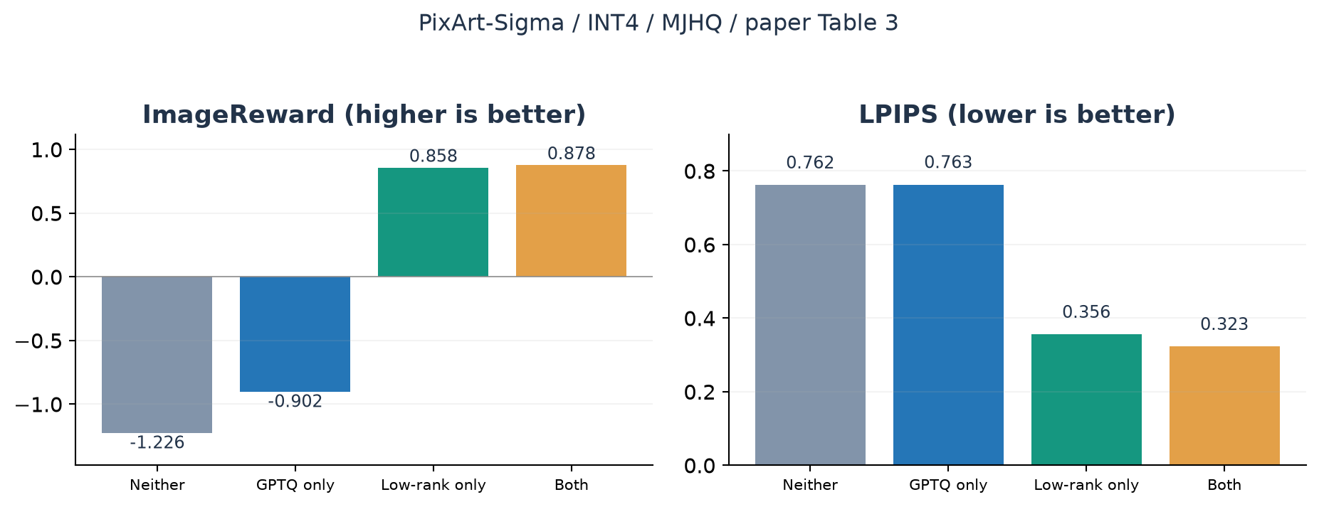
Figure 7 (redrawn from paper Table 3): PixArt-Sigma INT4 ablation on MJHQ. The four bars distinguish the contribution of the protected branch from residual-weight quantization. Negative ImageReward values are preserved rather than hidden by the plot scale.

The ablation is not uniformly monotonic across every model and format. On FLUX.1-dev NVFP4, GPTQ without the low-rank branch has LPIPS 0.204 and PSNR 21.5, versus 0.208 and 21.4 with both. ImageReward moves in the opposite direction, from 0.936 to 0.937. This is another reason to describe an accuracy-efficiency tradeoff rather than a guaranteed improvement from adding each component.

Table 3 also lists schnell’s BF16 ImageReward as 0.968, whereas Table 1 lists 0.938. The paper does not reconcile that baseline difference in the surrounding discussion. I avoid calculating a cross-table improvement using those incompatible baselines. A corrected table or a precise explanation of sampling differences would improve the presentation.

9.3 Latency: identify the denominator

Appendix Table 4 reports single-step FLUX latency of 657 ms for BF16, 282 ms for INT8, 212 ms for naive INT4, 250 ms for SVDQuant without Nunchaku, and 218 ms with Nunchaku. Direct calculation gives $250/212-1\approx17.9\%$ unfused overhead and $218/212-1\approx2.8\%$ remaining fused overhead relative to the naive INT4 reference.

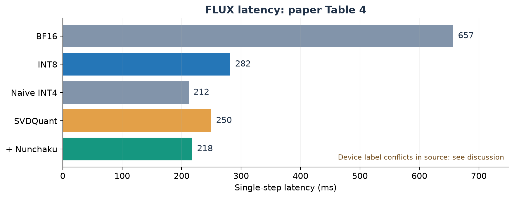
Figure 8 (redrawn from paper Table 4): reported single-step times. The appendix paragraph calls the device a laptop RTX 4090, while the caption calls it a desktop RTX 4090. I preserve the times but do not resolve this conflicting hardware attribution by guessing.

The 218 ms result is about 3.01 times faster than 657 ms BF16 and 1.29 times faster than 282 ms INT8. It is not a 3-fold improvement over naive INT4; that reference is slightly faster and serves as a useful lower-overhead target. Nunchaku recovers most of the speed that would otherwise be lost to the protective branch.

The much larger laptop speedup in the main paper includes avoiding per-layer CPU offload because the BF16 model does not fit in 16 GB. That is a legitimate practical benefit, but it compares different data-residency regimes. Figure 1’s 8.7-fold end-to-end result and Figure 8’s 10.1-fold result should not be presented as interchangeable kernel speedups. Text encoder and VAE costs matter for the end-to-end denominator, especially with a short-step sampler.

For a fixed unaffected fraction $1-f$ of execution time and a speedup $s$ on the optimized fraction, the simple Amdahl model gives

$$S_{\mathrm{total}}=\frac{1}{(1-f)+f/s}. \tag{14}$$

For example, if 80% of time benefits from a 3-fold acceleration, overall speedup is about 2.14-fold. This is an illustrative calculation, not an estimate fitted to the paper. It explains why the latency scope must accompany every reported multiplier.

10. Rank and precision are workload choices

The paper’s default rank 32 is a compromise. Appendix E.5 compares ranks 16, 32, and 64 on PixArt-Sigma, showing improved quality with increasing parameter and latency costs. The qualitative ablation in Figure 10 uses rank 64, so it should not be mistaken for an image comparison at the default rank used elsewhere.

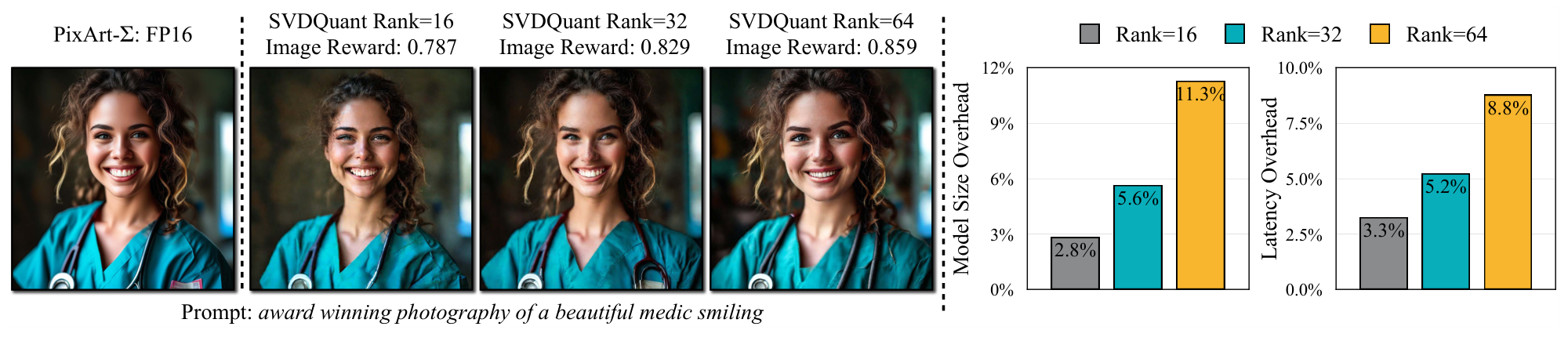
Figure 9 (paper Fig. 18): PixArt-Sigma examples and reported parameter/latency tradeoffs for different protected ranks. The figure illustrates a quality-cost tradeoff, not a universal justification for selecting rank 32 in every layer.

Increasing rank always reduces the unquantized SVD residual norm, but final image metrics need not improve monotonically. The residual quantization grid, calibration objective, trajectory dynamics, and finite-precision factors also change. Uniform rank is operationally simple; allocating rank per layer may improve the quality-cost frontier, but it requires a measured latency model rather than just a parameter budget.

Appendix E.6 explores lower bit widths. The authors report viable three-bit images in the studied cases but failure at two-bit settings such as W2A4 or W4A2. This does not imply that three-bit arithmetic has the same native acceleration path as the demonstrated INT4/NVFP4 engines. A numerical feasibility curve and a deployed throughput curve are separate experiments.

The bit-width comparison also changes quantization granularity: per-channel above four bits and group size 64 at four bits or below. It is useful as a comparison of practical configurations, but not a clean single-variable experiment on bit width. Any follow-up should report the format, grouping, scale storage, and protected rank alongside the nominal number of bits.

Algorithm 3. A controlled evaluation plan

This is my proposed experimental protocol, not an experiment executed for this review. It targets the ambiguities in the reported evidence rather than checking repository internals.

1. Fix model, sampler, steps, resolution, prompts, seeds, and guidance.
2. Reserve separate calibration and evaluation prompt sets.
3. Record all precision exceptions, rank choices, groups, and scales.
4. Compare quality metrics on paired outputs and distributional samples.
5. Report denoiser-only and complete-pipeline latency separately.
6. Measure GPU-resident and CPU-offloaded baselines as separate regimes.
7. Sweep protected rank and format with the same quality evaluation.
8. Repeat timing and report variability, peak memory, and warmup policy.
9. Publish a quality-memory-latency frontier with all exceptions labeled.

11. Limitations and failure boundaries

The main numerical boundary is spectral concentration. If smoothing produces a broad spectrum, a small protected branch cannot absorb enough difficult directions. If the input distribution changes materially, calibrated channel scales may also cease to be appropriate. The paper demonstrates useful robustness across two evaluation prompt sets, but that is not a stress test of all resolutions, guidance strengths, negative prompts, or adapter combinations.

A second boundary is the gap between local and global objectives. Frobenius residual energy does not encode which output directions are most important to the denoising trajectory. Layer-output MSE is more task-related, but still does not directly optimize human preference or prompt correctness. Successful images and favorable aggregate scores support the method empirically; they do not convert the local bound into an end-to-end guarantee.

A third boundary is the hardware path. INT4 and NVFP4 require suitable low-bit execution support, and the two fusion pairs depend on compatible tensor layouts and manageable resource use. Benefits measured on the paper’s NVIDIA devices should not be assigned to other accelerators without measurement. Adapter rank and batch shape may make the supposedly small branch less convenient to fuse.

Finally, the reported metrics have limited uncertainty information. Many aggregate improvements are convincing in size, particularly the prevention of PixArt INT4 collapse, but tiny differences such as LPIPS 0.257 versus 0.258 should not be given a strong ranking interpretation without variability estimates. Example images reveal possible failure modes; they do not estimate their frequency.

12. Critical analysis: what I would change next

12.1 Optimize protected rank for output sensitivity and latency

SVDQuant’s uniform rank keeps execution simple, but different layers need not have the same spectral concentration or downstream sensitivity. A promising extension would choose rank using a combination of residual output error and measured fused-kernel cost. The first test should compare uniform rank with a small discrete rank menu at equal peak memory and equal denoiser latency, keeping the calibration set fixed.

I would avoid claiming success solely from a lower sum of layer MSEs. The extension should be evaluated through complete denoising trajectories, including paired seed tests and difficult prompt categories. A layer whose error is amplified by later steps can deserve more rank than one with a larger raw weight norm. Conversely, increasing rank in a layer that pushes a fused kernel past an occupancy threshold can be a poor systems tradeoff even if its approximation improves.

12.2 Separate format, grouping, and the protection mechanism

NVFP4 uses a finer group size than the paper’s INT4 setting. Its quality advantage therefore does not identify the contribution of the floating-point grid alone. I would first perform an offline numerical factorial comparison across format, group size, GPTQ, and protected rank. This does not require every combination to have a fast hardware path; it isolates the numerical mechanism before selecting the deployable combinations.

The existing Table 3 already offers a useful warning against a simple additive story. GPTQ and the protected branch can improve different metrics by different amounts, and occasionally their combination is slightly worse on similarity. Reporting per-layer output errors alongside final image metrics would help determine whether these exceptions come from local approximation, calibration selection, or trajectory sensitivity.

12.3 Make the theoretical claims match the quantizers used

The core algebra is clean, but the residual-norm argument is a surrogate. A strengthened analysis would bound error per group and explicitly include scale quantization, clipping, high-precision factor rounding, and the nonuniform FP4 grid. It should also state the dependence of the regularity constant on the residual distribution instead of treating it as stable across transformations.

For the Gaussian illustration, the absolute-maximum correction discussed in Section 4 is straightforward. More importantly, learned residuals are not guaranteed independent, zero-mean Gaussian samples. Empirically measuring the ratio between maximum magnitude and Frobenius norm across layers and groups would show whether the theoretical intuition is relevant in the regimes where the method succeeds or fails.

12.4 Repair the evidence trail before strengthening the headline

The dimension-order typo, ImageReward prose/table mismatch, schnell baseline discrepancy, and Table 4 device conflict are individually repairable. Together they make a reader work harder to identify the exact experiment supporting a sentence. A versioned results sheet linking each figure and table to its model, sampler, prompt set, rank, numerical format, device, and timing scope would resolve much of this ambiguity.

I would also add a small error taxonomy for generated images: missing objects, text corruption, structural artifacts, and prompt relation failures. FID and learned rewards can hide such categories. The practical question is not only whether mean quality remains close, but whether a low-bit configuration introduces a new class of failures that matters to the intended application.

My assessment remains positive: the paper makes a compelling case for allocating a small high-precision budget to the most difficult component and then designing execution around shared tensors. The caveats narrow the claim and suggest useful experiments; they do not undermine the central algorithm-and-system argument.

13. Conclusion

SVDQuant is a good example of using low rank as a precision allocation tool. Smoothing relocates the problem, SVD extracts a compact high-energy component, residual quantization makes the main multiplication cheap, and Nunchaku reduces the memory cost of protecting that component. Each stage addresses a different bottleneck.

The strongest evidence is the combination of preserved generation quality in difficult four-bit settings and measured execution gains from fusion. The important qualifications are equally concrete: some operations remain high precision, calibration and GPTQ are part of the evaluated method, quality metrics do not all agree, and offload avoidance is a different source of speedup from a faster matrix product.

For my own work, the reusable design lesson is to evaluate an approximation in three spaces at once: the numerical subspace being protected, the tensors moved through memory, and the end-to-end behaviour the user observes. A good result in just one of those spaces is not sufficient.

References and resources

1. Li et al. SVDQuant, arXiv v4, including Sections 3-5 and Appendices A-F. Full text.
2. Authors’ project page, used for resource attribution; technical comparisons above follow the specified paper version.
3. DeepCompressor and Nunchaku, official resource entry points linked by the paper.

No model inference, calibration run, or independent performance reproduction was conducted for this review. Original figures are explicitly illustrative; redrawn data and cropped figures are attributed at their point of use.