ProRL: What Prolonged Reinforcement Learning Changes, and What Its Evidence Can Prove

Review date: 2026-09-29
Author: Zhongzhu Zhou
Paper reviewed: ProRL: Prolonged Reinforcement Learning Expands Reasoning Boundaries in Large Language Models
Paper authors: Mingjie Liu, Shizhe Diao, Ximing Lu, Jian Hu, Xin Dong, Yejin Choi, Jan Kautz, Yi Dong
arXiv: 2505.24864v1, 30 May 2025

1. The question I think this paper makes useful

A language model can improve in two visibly different ways. It may answer an already solvable question correctly more often, or it may begin solving questions for which previous sampling found no successful answer. ProRL asks whether sustained reinforcement learning can deliver the second kind of improvement, rather than merely the first. That is a useful empirical question, provided that the sampling budget and the definition of success remain explicit.

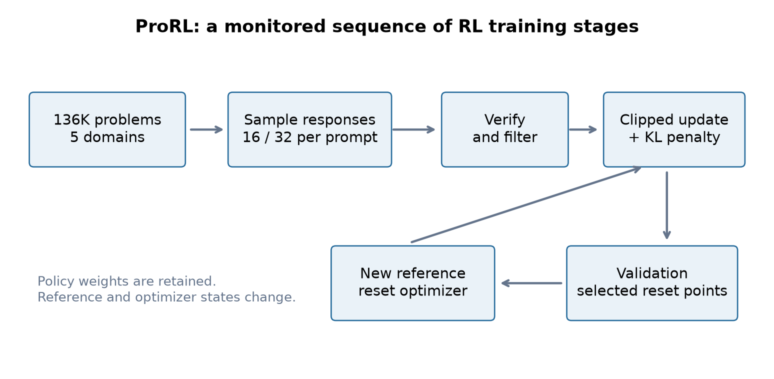
The paper starts from DeepSeek-R1-Distill-Qwen-1.5B, a model that already has substantial reasoning-oriented post-training. It then trains a generalist model on 136K verifiable problems in five domains, over more than 2,000 reported training steps and eight successive stages. The recipe combines group-relative policy optimization, asymmetric clipping, dynamic prompt filtering, a KL penalty, and resets of the reference policy and optimizer state. The final model is Nemotron-Research-Reasoning-Qwen-1.5B.

I find the strongest contribution to be a concrete counterexample to an overly broad pessimistic claim: the tested RL recipes do not invariably trade better single-sample accuracy for worse multi-sample coverage. ProRL improves both on several coding and puzzle settings, and it shows useful transfer to held-out task types and larger graph instances. But the paper also reports mathematical benchmarks where coverage falls, and domains where an intermediate checkpoint is better than the final checkpoint at large sampling budgets. Those results belong in the main interpretation, not in a footnote.

My reading separates three claims. Measured performance improves is strongly supported by the reported tables. A particular multi-stage recipe can maintain useful learning over a long run is supported by the training trajectory. Duration alone creates reasoning pathways absent from the base distribution requires stronger controls and a more careful definition of absence. Finite sampling cannot establish that a sequence has zero probability, and several ingredients change during this run.

2. Prerequisites: policy, reward, and the meaning of exploration

2.1 The policy is a distribution over answers

For a prompt $x$, let $y=(y_1,\ldots,y_T)$ be a generated response and let $\pi_\theta(y\mid x)$ denote its probability. Autoregressive factorization gives

$$\pi_\theta(y\mid x)=\prod_{t=1}^{T}\pi_\theta(y_t\mid x,y_{<t}),\qquad \log\pi_\theta(y\mid x)=\sum_{t=1}^{T}\log\pi_\theta(y_t\mid x,y_{<t}). \tag{1}$$

A verifier assigns a reward $R(x,y)$. With a fixed prompt distribution, the ideal reward objective is the expectation of that reward. Applying the identity $\nabla p=p\nabla\log p$ produces the score-function gradient:

$$J(\theta)=\mathbb E_{x,y\sim\pi_\theta}[R(x,y)],\qquad \nabla J=\mathbb E[R(x,y)\nabla_\theta\log\pi_\theta(y\mid x)]. \tag{2}$$

Equation (2) is explanatory background, not an additional theorem claimed by ProRL. It assumes that reward is treated as fixed with respect to the policy parameters during the update. A baseline independent of the sampled response can reduce gradient variance without changing the expected gradient; normalizing a sampled group is a practical estimator with its own behavior.

2.2 A correct verifier still defines only a particular target

The training rewards are not uniformly binary. Mathematics and STEM use binary signals, whereas code training uses the fraction of tests passed. Logic puzzles and instruction following use continuous rule-based rewards. For code, a syntax error, compilation failure, or a total execution timeout above five seconds yields zero under the described setup. Passing the available tests is a measurable objective; it is not a guarantee of semantic correctness on every possible input.

This matters for the debate about discovering solutions. A model can receive useful partial credit even when no sampled answer solves a whole problem. A claim derived under exclusively binary, all-or-nothing rewards does not automatically cover a recipe with continuous feedback. Conversely, an increase in average continuous reward must not be renamed an increase in strict problem-solving success without specifying a conversion rule.

Exploration has several meanings here. Higher sampling temperature increases diversity of generated tokens. A wider policy distribution may expose more candidate answers. More diverse answers can yield informative reward differences. None of these implications is automatic: increasing temperature can also generate incoherent responses, and verbal diversity can leave the underlying solution strategy unchanged. ProRL monitors entropy as a useful training statistic, but entropy is not a direct count of different correct algorithms.

3. From reward groups to usable policy updates

3.1 Why groups help, and where they lose signal

GRPO samples a group of responses to one prompt and uses relative rewards to construct advantages. For a group of size $G$, a compact notation for the paper’s normalization is

$$\bar R=\frac{1}{G}\sum_{i=1}^{G}R_i,\qquad s_R^2=\frac{1}{G}\sum_{i=1}^{G}(R_i-\bar R)^2,\qquad A_i=\frac{R_i-\bar R}{s_R}. \tag{3}$$

This notation uses population standard deviation for explanation; the article does not resolve every normalization convention. When all rewards coincide, $s_R=0$ and the expression needs special handling. ProRL describes removing prompts with uniformly successful or uniformly unsuccessful responses through dynamic sampling. I do not infer an undocumented numerical constant or a complete rule for equal non-binary rewards.

A small binary example makes the signal concrete. With rewards $(0,0,1,1)$, the mean is $0.5$ and population standard deviation is $0.5$, giving advantages $(-1,-1,1,1)$. With $(0,0,0,0)$, there is no relative outcome signal. The second group does not tell the method which failed answer was closer to correct. Continuous code-test rewards can distinguish some such cases, which is one reason the reward design belongs beside the optimization algorithm.

Under an illustrative independent Bernoulli model, let each response succeed with probability $p$. The group is informative in the narrow sense of containing both failures and successes unless all $G$ samples fail or all succeed. The events are disjoint, so

$$P_{\mathrm{mixed}}(p,G)=1-(1-p)^G-p^G. \tag{4}$$

For $p=0.01$, the probability is about $0.149$ with 16 samples and $0.275$ with 32. If collection repeatedly samples from this fixed population until a mixed group appears, the expected number of attempted groups is $1/P_{\mathrm{mixed}}$, roughly $6.73$ or $3.64$. These are explanatory calculations, not reported ProRL sampling costs. Real groups mix prompts of different difficulty, and partial-credit rewards change the model.

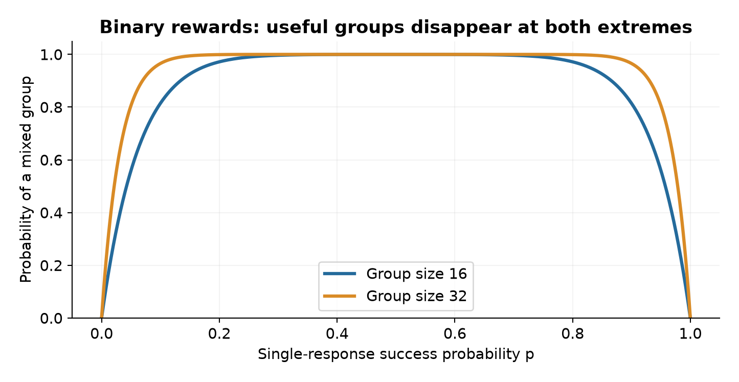
The boundary is important. Dynamic filtering cannot make an impossible-for-the-current-policy prompt informative by deleting its failures. A task may become learnable later through transfer from other prompts, partial rewards, or a changed sampling distribution. Thus filtering can serve as an implicit curriculum, but it can also repeatedly postpone the hardest part of the target distribution. The accepted groups and the rejected groups both matter when accounting for training work.

3.2 Asymmetric clipping changes the permitted incentive

Let $r_i=\pi_\theta(y_i\mid x)/\pi_{\mathrm{old}}(y_i\mid x)$ compare the updated and rollout policies. At the response level used in the paper’s exposition, the clipped surrogate is

$$\ell_i(\theta)=\min\left[r_iA_i,\; \operatorname{clip}(r_i,1-\epsilon_{\mathrm{low}},1+\epsilon_{\mathrm{high}})A_i\right]. \tag{5}$$

ProRL reports $\epsilon_{\mathrm{low}}=0.2$ and $\epsilon_{\mathrm{high}}=0.4$, following DAPO’s asymmetric construction. For a positive advantage, the objective stops increasing once the ratio reaches $1.4$, rather than the symmetric upper limit $1.2$. For a negative advantage, lowering the ratio beyond $0.8$ ceases to provide additional improvement through the clipped branch. The minimum and the sign of the advantage are both necessary to understand this behavior.

Clipping is a modification to the surrogate objective, not a hard constraint forcing every future probability ratio into an interval. Shared parameters and gradients from other examples can still move a ratio beyond the clipped range. The upper allowance is intended to make it easier to increase probabilities of useful low-probability outputs; it does not itself guarantee a particular entropy trajectory.

The paper’s equations are compact response-level descriptions, while its discussion refers to token probabilities. I preserve the conceptual objective rather than claiming that it specifies every token aggregation, masking, length normalization, or rollout-sampling correction. Those choices matter for long responses. Equation (5) describes a pedagogical surrogate for data generated by a frozen rollout policy; the displayed expectation in the paper is written with the current policy. It should not be interpreted as a complete executable training specification.

Algorithm 1. One informative-group update, summarized from the paper

Input: policy theta, rollout snapshot old, reference ref,
       task sampler, group size G, clipping bounds, KL weight beta
1. Draw prompts from the current multi-domain training mixture.
2. Generate G responses per prompt with the rollout policy.
3. Apply the task-specific verifier to each response.
4. Filter groups with accuracy entirely zero or entirely one,
   as described by the dynamic-sampling recipe.
5. Form relative advantages for retained, varying-reward groups.
6. Form the clipped surrogate and subtract the KL penalty.
7. Update theta with AdamW over the accepted rollout batch.
8. Record accepted and rejected work, entropy, length, and rewards.
Output: updated policy and training diagnostics

Steps 1-7 summarize the described procedure; the explicit rejected-work accounting in step 8 is my recommendation for interpretable compute reporting. Equal continuous-reward groups, the KL coefficient, and some update conventions remain unspecified in the reviewed paper. The pseudocode deliberately leaves those quantities as inputs instead of inventing values.

4. A moving KL anchor: what a reset actually changes

4.1 Regularization is not an entropy guarantee

The regularized objective in ProRL subtracts a divergence from a reference policy:

$$L(\theta)=L_{\mathrm{clip}}(\theta)-\beta D_{\mathrm{KL}}(\pi_\theta\Vert\pi_{\mathrm{ref}}),\qquad D_{\mathrm{KL}}(\pi\Vert q)=\sum_y\pi(y)\log\frac{\pi(y)}{q(y)}. \tag{6}$$

For a fixed prompt and compatible supports, expanding the logarithm exposes the relationship to entropy:

$$-D_{\mathrm{KL}}(\pi\Vert q) =-\sum_y\pi(y)\log\pi(y)+\sum_y\pi(y)\log q(y) =H(\pi)+\mathbb E_\pi[\log q(y)]. \tag{7}$$

The first term favors entropy, but the second favors outputs likely under the reference. A concentrated reference can support a concentrated updated policy. Therefore the empirical observation that KL helps preserve exploration in this run is plausible without implying a universal entropy floor. The starting reference is also a reasoning-distilled model, not an unadapted pretrained checkpoint; the paper explicitly distinguishes that context from recipes that remove KL during training from a weaker starting point.

The reference can eventually become restrictive. If the policy discovers useful answers that the fixed reference considers unlikely, their reward benefit must compete with a growing penalty. A reference reset changes that competition while retaining the policy’s learned weights.

4.2 A simple derivation explains the attraction of a moving reference

Consider a simplified distribution-level problem with fixed rewards and no clipping: maximize $\sum_y\pi(y)R(y)-\beta\sum_y\pi(y)\log[\pi(y)/q(y)]$ subject to probabilities summing to one. Introducing a Lagrange multiplier and setting the derivative for each outcome to zero gives

$$R(y)-\beta\left(\log\frac{\pi(y)}{q(y)}+1\right)+\lambda=0 \quad\Longrightarrow\quad \pi^*(y)=\frac{q(y)e^{R(y)/\beta}}{\sum_z q(z)e^{R(z)/\beta}}. \tag{8}$$

The derivation explains why the anchor matters: the reward tilts the reference distribution. It is not a closed-form solution to neural GRPO, which also has sampling, parameter sharing, clipping, and finite optimization steps. In the simplified setting, zero reference mass cannot acquire positive mass through this expression. With positive mass, an output may still be practically inaccessible because its probability is tiny.

At a reset time $s$, the mechanism can be written schematically as

$$\pi_{\mathrm{ref}}\leftarrow\pi_{\theta_s},\qquad \text{optimizer state}\leftarrow\text{fresh state},\qquad D_{\mathrm{KL}}(\pi_{\theta_s}\Vert\pi_{\mathrm{ref}})=0. \tag{9}$$

The final equality is exact only when the reference is an exact copy evaluated under the same distribution. Subsequent training can again diverge from this new anchor. The figure of KL across stages is consistent with this restart pattern, but the KL value after a reset is measured relative to a different reference. Adding or comparing such values as though they measured distance from the original base would be incorrect. KL is not a metric and does not supply a triangle-inequality bound on cumulative policy movement.

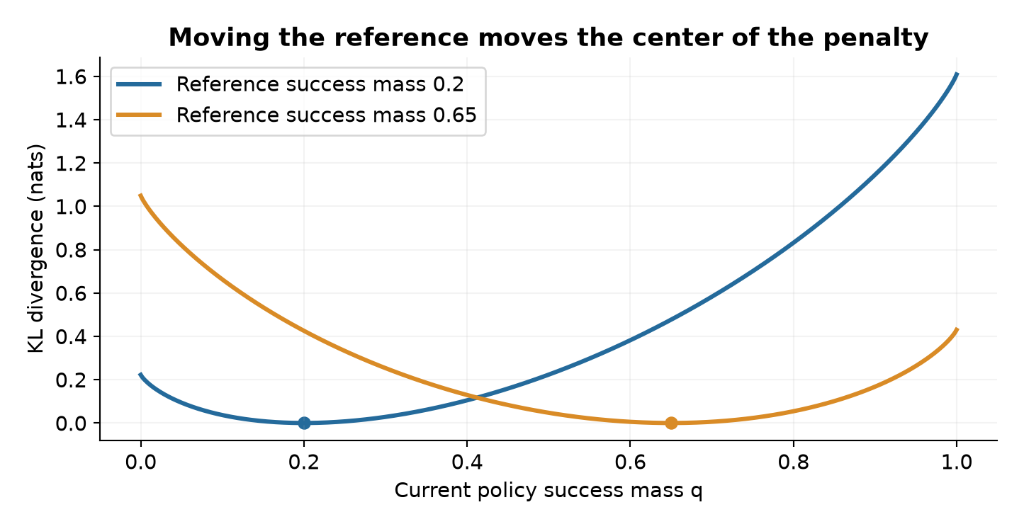
Resetting optimizer state is also a separate intervention. AdamW’s moving estimates of gradient moments affect the next update, even if model weights do not change. The paper couples reference reset with optimizer-state reset. Without separate controls, an improvement immediately after a reset cannot be attributed exclusively to the new KL reference.

Algorithm 2. Multi-stage continuation with monitored resets

Input: reasoning-distilled initial policy, validation blend,
       stage-specific data and sampling settings
1. Initialize the trainable policy and its reference snapshot.
2. Train with informative groups and the regularized objective.
3. Evaluate the monitored validation blend at checkpoints.
4. If the chosen monitoring rule detects degradation or plateau:
   a. Preserve the current policy weights.
   b. Copy a selected recent policy into the reference.
   c. Reinitialize optimizer state.
   d. Apply the next recorded stage configuration, if any.
5. Continue training and retain intermediate checkpoints.
6. Evaluate base, intermediate, and final models separately.
Output: a training history and models, not just one final score

This is a readable reconstruction of Sections 3.3 and Appendix E. The paper describes a validation-triggered decision, not a fully specified automatic plateau detector with a fixed threshold and patience. I therefore do not label the eight stages as a deterministic schedule that another reader could exactly reproduce from these steps alone.

5. The actual training intervention has eight stages

The 136K problem count comprises 40K mathematics, 24K code, 25K STEM, 37K logic puzzles, and 10K instruction-following examples. Initially only the first four domains are used; instruction following is added at stage 3. Data availability therefore changes the training distribution during the run.

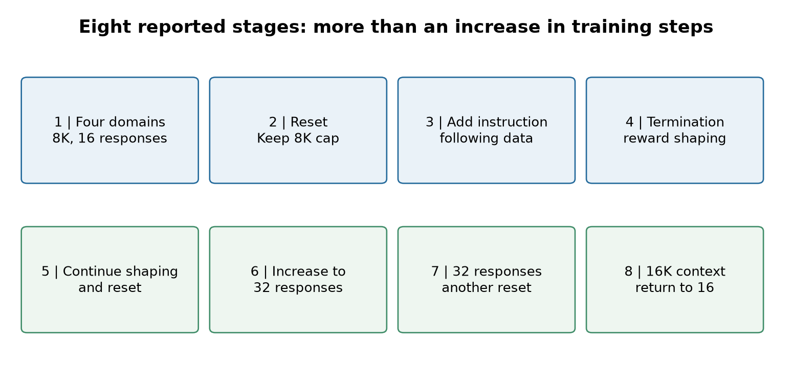
Stages 1 and 2 retain an 8K response budget; stage 2 follows a reset. Stage 3 adds instruction-following data, then encounters repeated answers and failure to terminate. Stages 4 and 5 add termination-related reward shaping. Stages 6 and 7 raise responses per prompt from 16 to 32 with further resets. Stage 8 extends the context budget to 16K and returns to 16 responses; the main text describes this final extension as roughly 200 steps.

The nominal setup uses rollout temperature 1.2, batch size 256, minibatch size 64, AdamW learning rate $2\times10^{-6}$, and four gradient updates per rollout step as described in Section 3.2. That section gives a context limit of 8096, whereas the narrative uses 8K. I retain the literal distinction rather than silently replacing it with 8192. Training is reported on four nodes with eight H100-80GB GPUs each, for approximately 16,000 GPU-hours.

Different stages use different response counts and lengths, and dynamic sampling discards some prompt groups. Section 11 therefore evaluates the cost in generated tokens and GPU-hours rather than treating each training step as an equal unit.

There is useful engineering judgment in the staged intervention. Keeping short responses early lowers cost and may discourage verbose failure modes; later increasing the limit can unlock tasks that benefit from longer traces. Adding a termination penalty addresses a specific pathological behavior. Increasing group size can improve reward comparison when successes are rare. However, these simultaneous improvements mean that the final-versus-intermediate comparison is not a pure experiment in elapsed RL duration.

6. Reading the headline results without changing the metric

6.1 Large gains, with a distinction between percentage points and percent

The main evaluation uses temperature 0.6, top-p 0.95, and a maximum response length of 32K. For mathematics, code, and STEM, the paper estimates pass@1 from 16 responses per prompt with binary evaluation rewards. Logic puzzles and instruction following instead report mean continuous verifier reward. The paper evaluates open models under its own stated evaluation settings.

Domain / benchmark aggregate	Distilled 1.5B base	ProRL 1.5B	Difference
Math average, Table 1	44.45	60.14	+15.69 points
Code average, Table 2	23.08	37.49	+14.41 points
GPQA, Table 3	15.86	41.78	+25.92 points
IFEval mean reward, Table 3	44.05	66.02	+21.97 points
Reasoning Gym mean reward, Table 3	4.24	59.06	+54.82 points

All values use the paper’s 0-100 display scale. Calling the math gain 15.69 percent would be ambiguous: the absolute difference is 15.69 percentage points, while the relative increase over 44.45 is about 35.3%. For continuous reward, I use score points rather than pretending the metric is a proportion of completely correct answers.

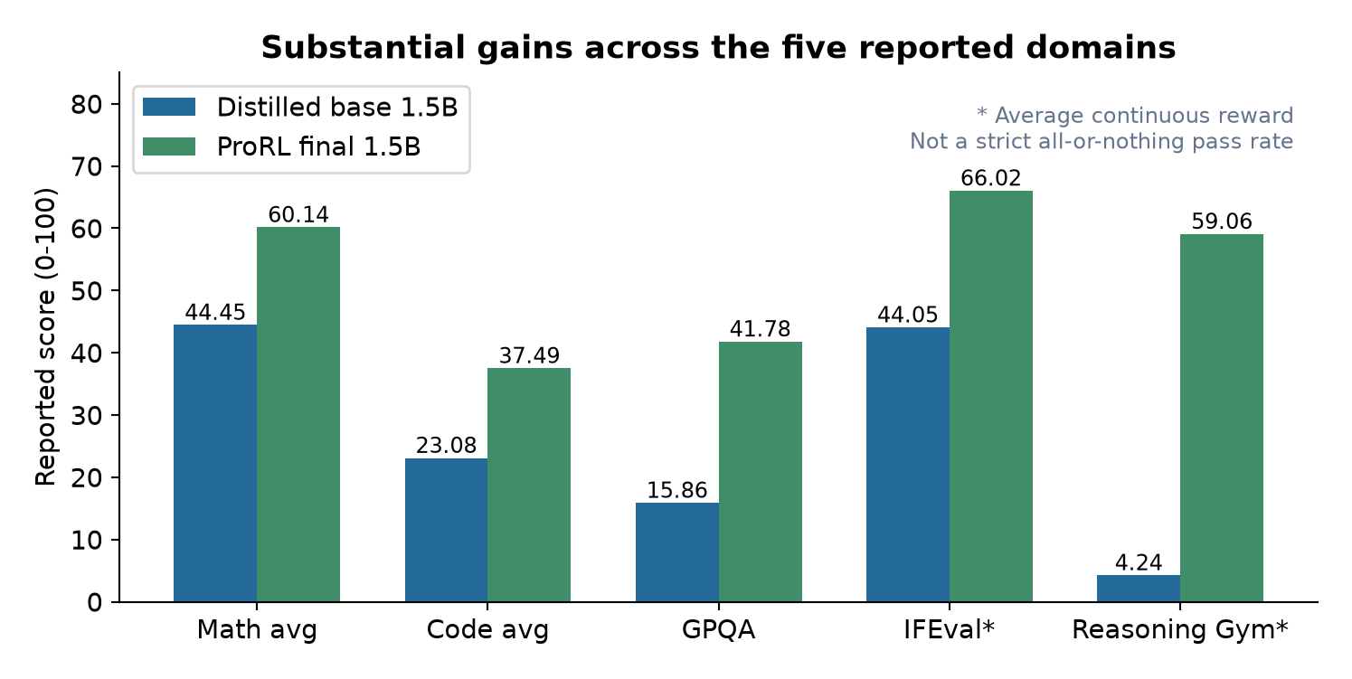
There are inconsistencies within the paper’s summary prose. The introduction lists math, code, STEM, and instruction-following gains of 14.7, 13.9, 25.1, and 18.1, while Sections 3-3.4 and the main tables support approximately 15.7, 14.4, 25.9, and 22.0. I use the tabulated values above and preserve the discrepancy. It is not resolved by switching from relative percentages to absolute points.

6.2 A generalist can beat a specialist average without winning everywhere

On math, ProRL’s 60.14 average exceeds DeepScaleR-1.5B’s 54.54 by 5.60 points. The prose reports a +4.6 gain, which does not match those table entries. On code, 37.49 exceeds DeepCoder-1.5B’s 30.96 by 6.53 points, consistent with the rounded +6.5 claim. The specialist baselines are valuable references, but their complete training budgets and data mixtures are not held constant in this comparison.

Individual results also resist a universal ranking. ProRL reaches 72.05 on HumanEvalPlus versus DeepCoder’s 73.40, despite winning the six-benchmark code average. Compared with the 7B distilled reference, ProRL has lower math average, 60.14 versus 63.19, and lower code average, 37.49 versus 41.39. It is higher on GPQA, IFEval, and Reasoning Gym under this evaluation. The accurate statement is competitive performance across several tasks with much fewer parameters, not a blanket replacement for a 7B model.

Table 5 provides another valuable boundary. ProRL scores 2.52 on the ARC category, compared with 3.42 for the 7B reference, although the table caption says it is superior across all reasoning tasks. Algebra improves to 97.21, while ARC remains extremely weak. A macro-summary of improvement can conceal qualitatively different remaining failure modes.

7. What pass@k measures, and how to estimate it

7.1 Success probability is prompt-specific

Let $p_x$ be the probability that one independently sampled response to prompt $x$ passes a specified binary verifier under a fixed decoding policy. All $k$ responses fail with probability $(1-p_x)^k$. Taking the complement and then averaging over prompts yields

$$\operatorname{pass@}k(x)=1-(1-p_x)^k,\qquad P_k=\mathbb E_x[1-(1-p_x)^k]. \tag{10}$$

This is an oracle-coverage metric: a correct response must exist in the sample set. It does not show that a deployment system can identify that response without a ground-truth verifier. Majority voting, a learned judge, and execution-based selection are different mechanisms, with different costs and error rates. Better pass@256 is informative about the search distribution even when it is not the best deployment choice.

Given $n$ sampled responses and $c$ observed successes, a standard finite-sample estimator counts the fraction of size-$k$ subsets containing at least one success:

$$\widehat{\operatorname{pass@}k}(x) =1-\frac{\binom{n-c}{k}}{\binom{n}{k}},\qquad 1\leq k\leq n. \tag{11}$$

There are $\binom{n}{k}$ possible subsets; $\binom{n-c}{k}$ contain failures only. When $n-c<k$, the numerator is zero. When $k=n$, the estimator is one if any sample succeeded and zero otherwise. This derivation explains the metric I would request in a replication protocol; the ProRL text does not provide enough detail to certify that every continuous-reward plot uses this exact binary estimator.

Algorithm 3. Transparent binary coverage evaluation

Input: fixed prompts, model, decoding settings, verifier, n, K
1. Freeze the prompt list, model checkpoint, and decoding settings.
2. For each prompt, collect n separately sampled responses.
3. Save binary success, parse status, length, and verifier outcome.
4. Let c be the number of successful responses for that prompt.
5. For each k in K with 1 <= k <= n:
   a. If n-c < k, assign estimated pass@k = 1.
   b. Otherwise use 1 - choose(n-c,k) / choose(n,k).
6. Average the per-prompt estimates with declared task weights.
7. Resample prompts for uncertainty estimates; keep each prompt's
   responses together when computing paired model differences.
Output: coverage curves, uncertainty, and an explicit metric definition

This is a proposed evaluation protocol, not a claim that I ran the authors’ model. Keeping responses together in a prompt-level bootstrap avoids treating many attempts at one question as many independent questions. It does not address all dependence between related generated puzzles; task families may need an additional grouping level.

7.2 A higher mean does not determine high-budget coverage

The function $f_k(p)=1-(1-p)^k$ is concave for integer $k\geq2$. Its second derivative is $-k(k-1)(1-p)^{k-2}$, which is nonpositive. Consequently, equal-mean success distributions can have different coverage. If every prompt has $p=0.4$, pass@2 is 0.64. If half have $p=0.8$ and half have $p=0$, mean pass@1 remains 0.4 but pass@2 is only 0.48. The second system concentrates skill on a subset of questions.

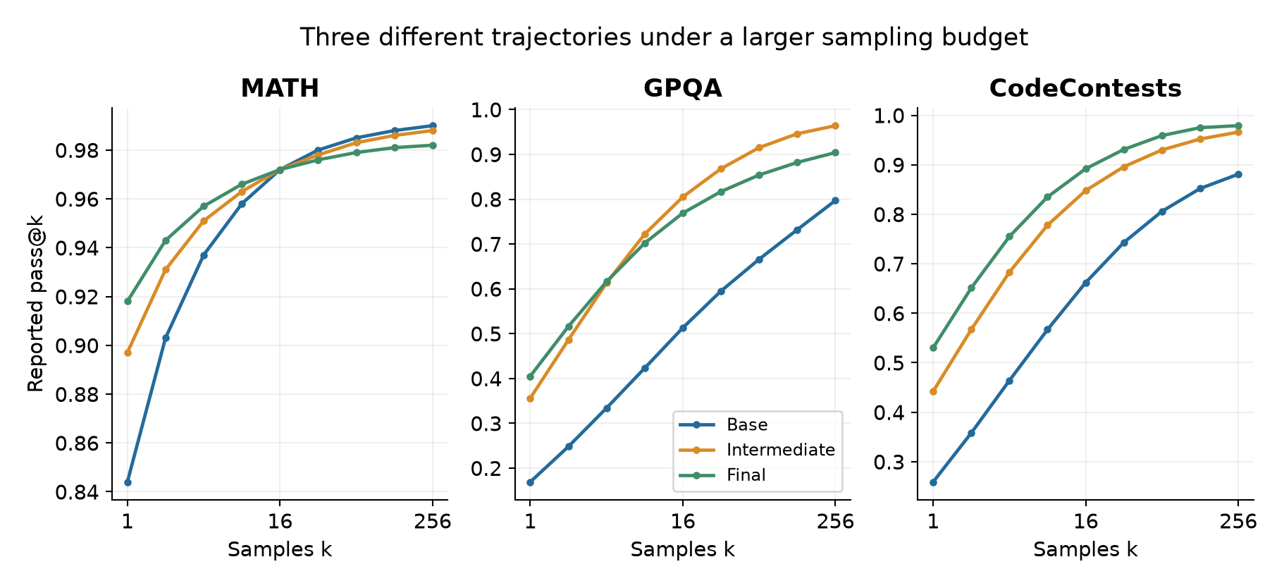
The paper’s Figure 4 illustrates why intermediate checkpoints should be retained. On MATH, the final model improves pass@1 from 0.844 to 0.918, yet pass@256 falls from 0.990 to 0.982. On GPQA, final pass@1 is 0.405 versus intermediate 0.356, while final pass@256 is 0.904 versus intermediate 0.964. On CodeContests, pass@256 increases from base 0.881 to intermediate 0.966 to final 0.979. These are three different trade-offs, not one monotonic story.

The displayed values come from the separate 256-response analysis. They do not exactly reproduce the earlier 16-response table estimates. In some coding cases the differences are substantial: APPS in Table 2 is 20.95/41.99 for base/final, while Figure 11 shows 0.292/0.583 at k=1. The paper does not reconcile this discrepancy. I keep the two evaluation summaries separate and do not attribute every difference to sampling noise without the underlying prompt lists and counts.

8. Generalization is real evidence, but its type matters

8.1 New task types and harder instances ask different questions

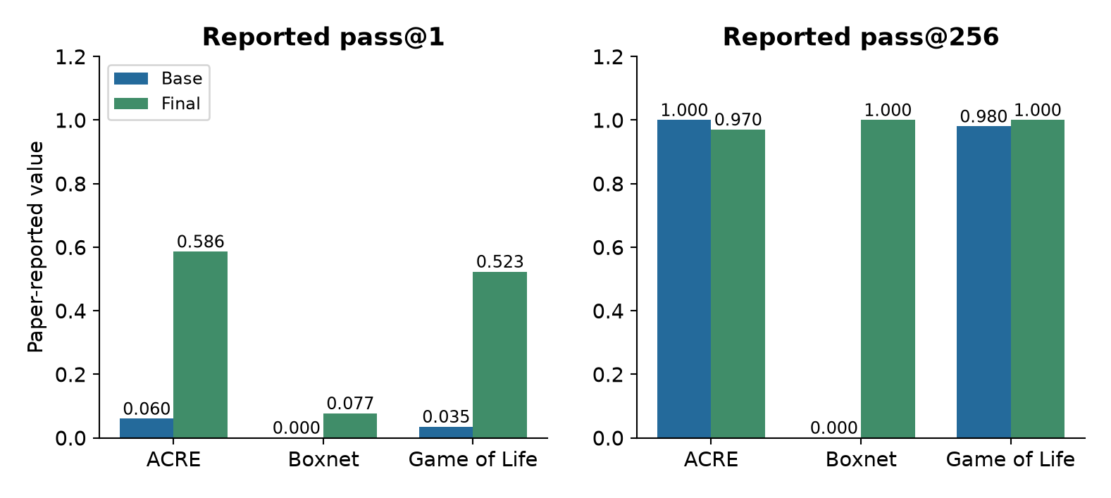
The paper evaluates three named held-out Reasoning Gym tasks in Table 3: ACRE, Boxnet, and Game of Life halting. Reported main-evaluation scores increase from 5.99 to 58.57, 0.00 to 7.91, and 3.49 to 52.29 respectively. These results support transfer beyond the task types explicitly used in training. They do not establish that every underlying concept or surface format was absent from pretraining.

The separate multi-sample analysis adds important qualifications. Figure 10 shows ACRE base/final pass@256 of 1.000/0.970, despite a large improvement at k=1. Boxnet improves from 0.000 to 1.000 at k=256, and Game of Life halting from 0.980 to 1.000. The final Boxnet model’s 0.077 at k=1 is still a low single-response success rate under the plotted measure. Describing this as universally reliable planning would discard the sampling budget that makes the result impressive.

The graph-coloring experiment instead changes difficulty within a task family. Training uses graphs with 10 vertices; evaluation includes larger graphs. Figure 12 shows final pass@1 dropping from 0.425 at 13 vertices to 0.102 at 15, 0.012 at 18, and 0.008 at 20. The larger sampling budget recovers much of the measured coverage, but the low single-sample rate remains relevant. Transfer to larger instances is meaningful; it is distinct from transfer to a new task family and from discovering an algorithm with a known complexity guarantee.

Appendix C makes the format burden visible. Graph coloring requests a JSON vertex-to-color map, family relationships requests a single relationship word, and Boxnet requests a sequence of JSON action plans subject to movement and conflict constraints. These are data examples in the paper, not instructions for the reader. Correct formatting and valid planning interact: a structurally valid plan can still be wrong, while a correct informal description can be rejected by a strict parser.

8.2 Zero observations are not proof of zero probability

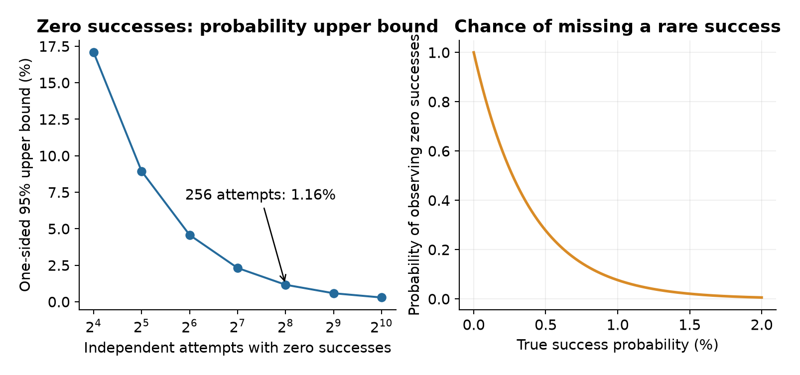
Suppose a fixed prompt yields no successful response in $n$ independent trials. For an underlying success probability $p$, the chance of this event is $(1-p)^n$. Solving $(1-p)^n=\alpha$ gives a one-sided confidence limit:

$$p_{\mathrm{upper}}=1-\alpha^{1/n}. \quad\text{For }n=256,\;\alpha=0.05:\quad p_{\mathrm{upper}}\approx0.01163. \tag{12}$$

Thus zero successes in 256 trials is compatible with a true per-attempt probability up to roughly 1.16% at this confidence level, under the stated assumptions. The small-probability approximation $-\log(0.05)/256\approx3/256$ gives the familiar rule-of-three intuition. This is an explanatory bound for one prompt, not a confidence interval I computed from unavailable ProRL raw samples.

For a genuinely rare success rate of 0.1%, the chance of observing no success in 256 trials is about 77.4%. A trained model can make such a success practically accessible while both models still assign it positive probability. That can be an enormous engineering improvement. We need not turn it into a claim about mathematical support to value it.

The actual decoding distribution matters too. Temperature and nucleus truncation modify which responses can be sampled; a top-p policy can remove paths that retain positive probability in the underlying softmax model. A careful claim should therefore identify the model checkpoint, decoding settings, response limit, prompt, and verifier. Here the defensible language is that the base did not solve the observed instances under the tested budget and protocol, while the trained model did.

9. Re-deriving the mean-variance bound

Section 4.4 cites a bound connecting the distribution of per-prompt success probabilities to aggregate pass@k. Its interpretation is easiest when the assumptions are explicit. Let $p_x\in[0,1]$, $\mu=\mathbb E[p_x]$, and $\sigma^2=\operatorname{Var}(p_x)$. Write $q_x=1-p_x$. For $k\geq2$, convexity of $z^{k/2}$ on nonnegative $z$ gives

$$\mathbb E[q_x^k]=\mathbb E[(q_x^2)^{k/2}] \geq (\mathbb E[q_x^2])^{k/2}. \tag{13}$$

Expanding the second moment then gives

$$\begin{aligned} \mathbb E[q_x^2] &=\mathbb E[(1-p_x)^2]\\ &=1-2\mu+\mathbb E[p_x^2]\\ &=(1-\mu)^2+\sigma^2,\\ P_k&\leq1-\left[(1-\mu)^2+\sigma^2\right]^{k/2}. \end{aligned} \tag{14}$$

For k=2 the bound is exact; at larger k it can be loose. It should not be applied to k=1 with the same inequality direction. Increasing the mean while holding the variance fixed raises the upper bound; increasing the variance while holding the mean fixed lowers it. This statement is about a bound, not a guarantee that an actual model’s pass@k must move in the same direction.

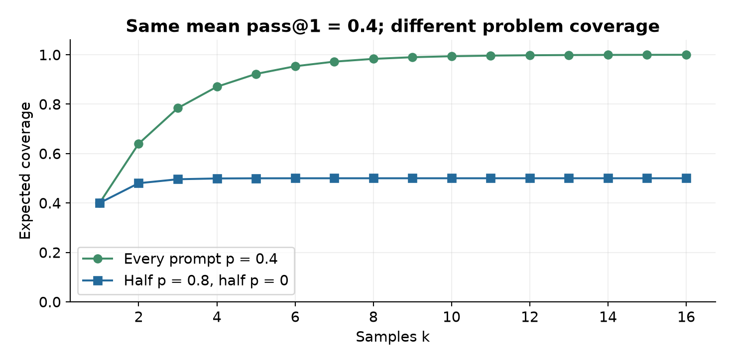
In the heterogeneous example from Section 7, $\mu=0.4$ and $\sigma^2=0.16$. Equation (14) gives pass@2 equal to $1-(0.36+0.16)=0.48$, matching direct calculation. At large k, actual coverage remains near 0.5 because half the prompts have zero success probability. Yet the bound tends toward one. This simple example shows why an upper bound alone cannot certify broad generalization.

The paper displays per-prompt distributions for several domains and argues that the mean shifts rightward enough to outweigh diversity losses. Those plots are useful descriptive evidence. Their smooth curves, however, do not remove finite-response estimation noise, and a fitted density is not an independent set of observations. The observed histogram is a distribution of estimated probabilities; it combines differences among prompts with uncertainty in each estimated probability.

10. What I would preserve when trying to reproduce the scientific result

Reproducibility here concerns the experiment’s meaning: which comparison a result supports. It does not require treating a repository as a substitute for the paper. The most useful specification would preserve the following items alongside the released model.

Item	Why it changes the conclusion
Initial distilled checkpoint and all selected checkpoints	Establishes the actual starting capability and exposes regression after intermediate stages
Prompt splits and task-generator settings	Separates new instances, larger instances, and held-out task types
Reward definitions and parse outcomes	Distinguishes formatting gains, partial credit, and full problem success
Stage boundaries and reset triggers	Makes the adaptive intervention understandable rather than labeling every difference as duration
KL weight and aggregation conventions	Determines the regularization strength and update behavior
Accepted and discarded rollouts, tokens, GPU-hours	Allows compute-matched comparison across changing group sizes and lengths
Model-by-prompt result matrices	Supports paired coverage estimates and uncertainty for rare successes

The paper reports the starting model, nominal training hyperparameters, data counts, stage descriptions, and many task-level plots. It does not provide a fully specified reset detector or a clearly stated KL coefficient in the reviewed text. It also states that the validation blend includes subsets from AIME2024, Codeforces, GPQA, IFEval, and graph coloring, drawn from evaluation benchmarks. That does not prove that final reported examples were directly trained on. It does mean that the distinction between monitoring data and a final untouched test set needs to be documented carefully.

For a future controlled experiment, I would start with the same initial checkpoint and data mixture in each branch, allocate equal generated-token budgets, and vary reference reset and optimizer reset separately. The no-reset branch should receive comparable hyperparameter tuning, not an intentionally poor fixed anchor. A separate branch would hold data, group size, and response budget fixed while increasing training duration. Those are proposed experiments, not completed replications.

11. Training and deployment budgets answer different questions

The paper reports four nodes with eight H100 80GB GPUs per node and approximately 16K GPU-hours. Dividing that aggregate by 32 GPUs yields roughly 500 hours if all GPUs were continuously occupied. This is an accounting conversion, not a measured wall-clock duration. It excludes any inference about utilization, engineering effort, failed runs, or the cost of data preparation.

A better unit for comparing RL recipes is often generated tokens, together with verifier cost and optimizer work. If an accepted prompt requires $G$ responses of mean length $L$, and a fraction $a$ of sampled prompt groups is accepted, a simplified rollout-token estimate for $B$ accepted prompts is

$$C_{\mathrm{rollout}}\approx\frac{BGL}{a}. \tag{15}$$

This is a planning approximation, not a measured ProRL scaling law. Response lengths and acceptance rates depend on the prompt, and some groups may be reused or collected under different scheduling rules. Nevertheless, the equation makes an important cost visible: doubling group size does not simply double useful gradient information. At $p=0.01$, the binary mixed-group model from Section 3 gives $a\approx0.149$ for $G=16$ and $a\approx0.275$ for $G=32$. Expected responses per accepted group are then about 108 and 116. Larger groups reduce the number of resampled prompts but still increase responses per accepted group slightly under these assumptions. They may improve estimation or reveal rarer successes, but that benefit needs measurement.

The same distinction matters at deployment. A model that solves a task with at least one of 256 samples is valuable only if a downstream system can recognize and select the successful sample at an acceptable cost. Code with reliable executable tests offers one route. A scientific question without a trusted verifier offers a much weaker route: oracle pass@256 does not directly become user-facing accuracy. Majority voting, reranking, and verifier selection each define another deployed policy and should be evaluated explicitly.

For an application with a strict one-response latency budget, the main-table accuracy gains may matter more than the tail of a pass@k curve. For an offline search application, coverage and verifier reliability may matter more. ProRL does not eliminate that tradeoff. It provides checkpoints and evidence that make the tradeoff more favorable on some tasks, while its GPQA and MATH500 curves show that a final checkpoint need not dominate at every budget.

12. Limitations of the evidence and of this review

Causal attribution is incomplete. Training duration, data mixture, group size, termination incentives, context allowance, reference resets, and optimizer resets change across the run. The paper demonstrates the complete recipe. It does not isolate a general causal effect of duration or prove that every reset component is necessary.

The starting point is a particular distilled model. DeepSeek-R1-Distill-Qwen-1.5B has already benefited from reasoning-oriented supervision. Results do not automatically extend to a raw pretrained model, other sizes, or other distillation histories. The reported comparisons are useful benchmarks, but they are not all equal-compute training experiments.

Sampling and reward semantics limit capability claims. Zero successes in 256 trials is informative but not proof of zero success probability. Continuous puzzle rewards are not interchangeable with binary solution events. The discrepancy between main-table and appendix sampling numbers needs clarification before combining them into a single quantitative narrative.

Uncertainty is underdeveloped. The reviewed evidence does not provide the multi-seed, compute-matched study needed to estimate recipe robustness. Per-task curves help reveal heterogeneity, but selected plots cannot substitute for uncertainty over model training and task sampling.

This reading is not a replication. All model-performance numbers above come from the paper. The plotted probability examples and bound derivations are explanatory calculations under stated assumptions. They do not establish new empirical results. The released weights are a useful resource; this article does not infer unrevealed training settings from them.

13. Independent critical analysis: what would change my mind?

13.1 Treat the reasoning frontier as an operational object

The phrase “new reasoning pathway” can refer to a new textual trace, a newly observed solution, a new algorithmic strategy, or probability mass on a sequence that was previously impossible. Those are different claims. ProRL directly measures the first two more easily than the last two. A softmax language model can assign extremely small but nonzero probability to many strings; a finite sample cannot establish literal support expansion over that space.

An operational frontier is more useful: the set of tasks solved with a specified decoder, verifier, response budget, and token budget. Under that definition, moving a task from an undetectably rare success rate to a practical one is a meaningful capability gain even if mathematical support never changes. We should not dismiss that gain as “only sampling.” We should also not use it to claim that the starting distribution contained no relevant behavior. The scientific disagreement becomes more tractable when the same operational frontier is measured on both sides.

13.2 Separate reasoning, formatting, and verifier interaction

Appendix F.1 shows a base response that returns a boxed answer where the puzzle expects an answer tag. That observation matters because measured success can be factored into at least two parts. Let $F$ be an event that an answer is accepted by the parser, and $C$ be semantic correctness conditional on successful parsing. Then, for a verifier that rejects unparseable responses,

$$P(\mathrm{accepted\ correct})=P(F)P(C\mid F). \tag{16}$$

Raising either term improves the score. Learning an output contract is useful learning, especially for an agent that must interact with tools. But it should be distinguished from acquiring a new solution algorithm. I would report the parse rate, correctness among parsed answers, and the original strict score together. A separately documented, semantics-preserving parser repair could reveal how much improvement survives when obvious formatting differences are neutralized. It must be designed before inspecting which repair favors which model, and it must not silently reinterpret wrong answers as correct ones.

The paper’s Creativity Index is also indirect evidence. It measures overlap against Dolma, not against the entire undisclosed pretraining and distillation history of the starting model. Lower overlap is compatible with novel wording, different formatting, or different solution structure. It is not by itself proof of algorithmic novelty or absence from training. I would pair that metric with matched-problem strategy annotations and counterfactual tests where a strategy’s defining step is required to change.

13.3 A reset can help without explaining all the gains

The moving KL anchor is a plausible answer to a concrete optimization problem: an increasingly strong policy can become costly to move away from an increasingly obsolete reference. Resetting the anchor removes that accumulated penalty while keeping learned weights. Resetting optimizer state may also alter the next updates. Either mechanism can help training continue, but a combined reset does not tell us their separate contributions.

A minimal factorial comparison would cross reference reset on/off with optimizer reset on/off under a fixed data mixture and token budget. A second comparison would vary the context allowance while keeping both reset choices fixed. The goal is not to demand every possible experiment before accepting the paper. It is to identify which extra experiment would most efficiently turn a working recipe into a more portable principle.

13.4 A decision protocol for stronger claims

The strongest next experiment would make the rules for choosing checkpoints and declaring expansion explicit before looking at the final test set. Repeatedly monitoring public benchmarks can encourage adaptive choices that fit those benchmarks, even without directly training on their exact examples. An untouched holdout and a recorded selection rule make that concern testable.

Algorithm 4. Proposed evaluation protocol, not an author-reported experiment

1. Freeze held-out task families and define binary success events.
2. Predeclare token budgets, sample counts, decoders, and selectors.
3. Select checkpoints using a separate validation set only.
4. Evaluate every selected model on the same held-out prompts.
5. Record parse rates, partial credit, and full success separately.
6. Estimate paired changes in pass@1 and coverage with uncertainty.
7. Compare training branches at equal generated-token budgets.
8. Report regressions and intermediate-checkpoint wins explicitly.

If this protocol showed a reproducible gain across several starting models, with stable or better high-budget coverage after neutralizing superficial format failures, I would have substantially more confidence in a broad reasoning-expansion claim. If most gains disappeared after those controls, the practical recipe could still be valuable, but its mechanism would be different from the headline interpretation.

14. Conclusion

ProRL is persuasive evidence that sustained, carefully managed RL can improve a small distilled model well beyond its initial measured performance. Its most informative details are the moving regularization anchor, the changing training stages, and the task-dependent pass@k curves. Together they show why neither “RL only sharpens existing answers” nor “longer RL always creates new reasoning” is an adequate summary.

The useful conclusion is conditional: this multi-stage recipe improves accuracy and expands measured coverage on several demanding tasks, while some high-budget capabilities regress and some apparent gains include output-format learning. The next step is to test that conclusion with fixed-budget controls, explicit reward semantics, and untouched held-out tasks. That would clarify which part of ProRL is a robust training principle and which part depends on this particular model, data mixture, and evaluation setting.

References and resource links

1. Mingjie Liu, Shizhe Diao, Ximing Lu, Jian Hu, Xin Dong, Yejin Choi, Jan Kautz, and Yi Dong. ProRL: Prolonged Reinforcement Learning Expands Reasoning Boundaries in Large Language Models, 2025. Primary source for every reported training and benchmark result; Sections 2-4 and Appendices A-F were read in full.
2. NVIDIA. Nemotron-Research-Reasoning-Qwen-1.5B. Official model resource, linked as released weights.
3. Yang Yue and colleagues. Does Reinforcement Learning Really Incentivize Reasoning Capacity in LLMs Beyond the Base Model?. Related counterpoint and a future reading candidate; its later versions are not used to retroactively change ProRL v1’s measurements.
4. Andrew Zhao and colleagues. Absolute Zero: Reinforced Self-play Reasoning with Zero Data. Related future reading on co-evolving task generation and solving; not an experimental baseline in this review.

Figures 1-9 are original explanatory diagrams or redrawings with their sources identified in the captions.