ACE: How Agents Accumulate Useful Context Without Rewriting It Away

Review date: September 28, 2026
Author: Zhongzhu Zhou
Paper reviewed: Agentic Context Engineering: Evolving Contexts for Self-Improving Language Models
Paper authors: Qizheng Zhang, Changran Hu, Shubhangi Upasani, Boyuan Ma, Fenglu Hong, Vamsidhar Kamanuru, Jay Rainton, Chen Wu, Mengmeng Ji, Hanchen Li, Urmish Thakker, James Zou, Kunle Olukotun
Version: arXiv:2510.04618v3, March 29, 2026
Sources: Versioned paper, author project, official resource
Reading scope: All 32 pages, including the additional models, cost tables, corruption studies and example prompts. Reported results below belong to the paper. Equations, toy examples and proposed evaluations are explanatory analysis, not new benchmark results.

1. The problem is keeping the right lesson

An agent completes a task, observes a failure, and writes a useful lesson. That sounds like improvement. The difficulty appears fifty tasks later: a helpful exception may have disappeared during repeated summarization, while a confidently stated mistake has survived. A system needs a policy for changing its accumulated context, not just a place to put more text.

ACE addresses this problem with a structured playbook. A Generator uses the current playbook to attempt a task. A Reflector diagnoses what the trajectory teaches. A Curator proposes a small addition, and a deterministic operation incorporates it into the existing collection. Earlier entries do not need to be regenerated merely because the latest task produced one new insight. The framework also tracks feedback about individual entries and refines redundant material.

This is a useful example of agent improvement outside model weights. It is narrower than allowing an agent to rewrite its entire harness: the central object being updated is contextual knowledge, while the surrounding generation, reflection and curation process is specified in advance. That distinction helps connect ACE to the broader self-improvement literature without attributing capabilities it does not establish.

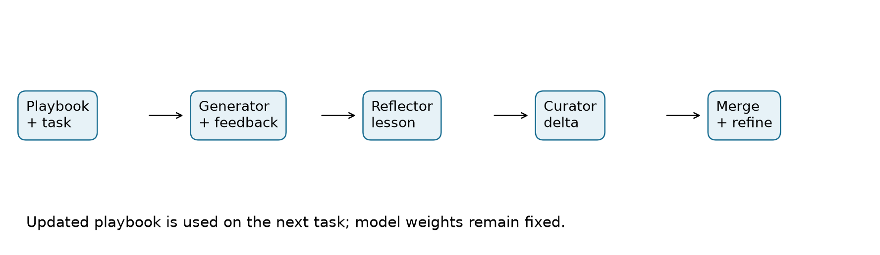
My reading has two conclusions. First, preserving detailed, reusable knowledge can matter more than finding a single elegant instruction. Second, retention is valuable only when the retained material is reliable and applicable. The paper’s own label-free classification failures, corruption experiment and longer evaluation inputs make that second point concrete. A larger memory is neither a guarantee of better judgment nor free computation.

2. Prerequisites: what is actually learning?

2.1 Parameters, context and a persistent state

Let a language model have fixed parameters $\theta$. On task $x_t$, its answer and trajectory depend on both the task and the context assembled from a playbook $P_t$. The following notation is my abstraction of ACE, rather than an equation claimed by the paper:

$$(\hat y_t,\tau_t)\sim p_\theta(\cdot\mid x_t,C(P_t)),\qquad P_{t+1}=U(P_t,\tau_t,f_t). \tag{1}$$

Here $\tau_t$ contains the interaction history, $f_t$ is available feedback, $C$ formats the playbook into model input, and $U$ is the context-update process. The model can behave differently tomorrow because $P_t$ changed, even when $\theta$ did not. This is adaptation of the surrounding system. It does not imply that the base model has permanently acquired the same capability in a fresh, empty context.

The distinction also separates ACE from retrieval alone. A retrieval system chooses existing material for the current question. ACE additionally decides what experience should become reusable material for later questions. Retrieval could be combined with that memory, but storing lessons and selecting lessons are different decisions. An unfiltered full playbook may contain relevant advice, obsolete details and mutually incompatible exceptions at the same time.

Consider a task involving two business records with identical display names. A raw transcript preserves the entire incident. A generic instruction says to be careful with identity. A useful playbook entry instead identifies the stable identifier to join on and the condition under which a display name is ambiguous. The third representation compresses a trajectory into a reusable procedure while retaining the detail that explains the failure. This is an illustrative example, not one of the paper’s measured tasks.

2.2 What counts as feedback?

A standard answer, a failed task check, an exception from a tool and the model’s own judgment carry different information. A tool exception can confirm that an argument was invalid, but successful execution does not establish that the task was completed correctly. A classifier can produce a well-formed label that is semantically wrong. A reflection procedure must therefore distinguish syntactic success from task success.

The paper’s “no ground-truth labels” setting removes one feedback source. It does not remove all external evidence: interactive environments can still report outcomes. Conversely, online adaptation with labels means the label is available after the prediction for updating the next state. It must not be inserted before the current prediction is scored. These distinctions explain why one feedback regime can help AppWorld while hurting FiNER.

2.3 Offline adaptation versus a moving online system

Offline adaptation builds a playbook on training examples and evaluates the resulting artifact on held-out tasks. Multiple passes can revisit training experience. Online adaptation predicts a test example, receives permitted feedback, updates the playbook, and moves on. Its score describes a changing system over a particular task sequence.

A compact expression for this sequential, or prequential, score is

$$\widehat A_{\mathrm{online}}= \frac{1}{T}\sum_{t=1}^{T} \mathbf 1\{\hat y_t(P_t)=y_t\}. \tag{2}$$

The subscript $t$ on $P_t$ matters. A frozen final playbook evaluated on the same examples answers a different question. If later tasks closely resemble earlier ones, the ordering is itself an adaptation opportunity. The paper uses the same shuffled test order across compared methods; repeated independent orders would additionally reveal how much the result depends on that particular sequence.

3. Why monolithic rewriting is fragile

3.1 Brevity bias loses conditions

A short instruction can express a broad principle, but many operational lessons depend on conditions. A rule about reading all pages of a result differs from a rule about stopping when a cursor is absent. Removing the termination condition can turn useful guidance into an endless loop; retaining a fixed page count can silently omit records. Detail has functional value when it distinguishes the successful procedure from a plausible wrong one.

ACE’s motivation is therefore not that concise writing is bad. It is that optimizing for a compact, polished summary can erase rare but useful exceptions. A good context representation should preserve the smallest actionable unit, including when it applies. The alternative is to retain raw trajectories, which protects details but spends more input tokens and leaves the Generator to rediscover their lessons.

3.2 Context collapse is a visible example, not a universal rate

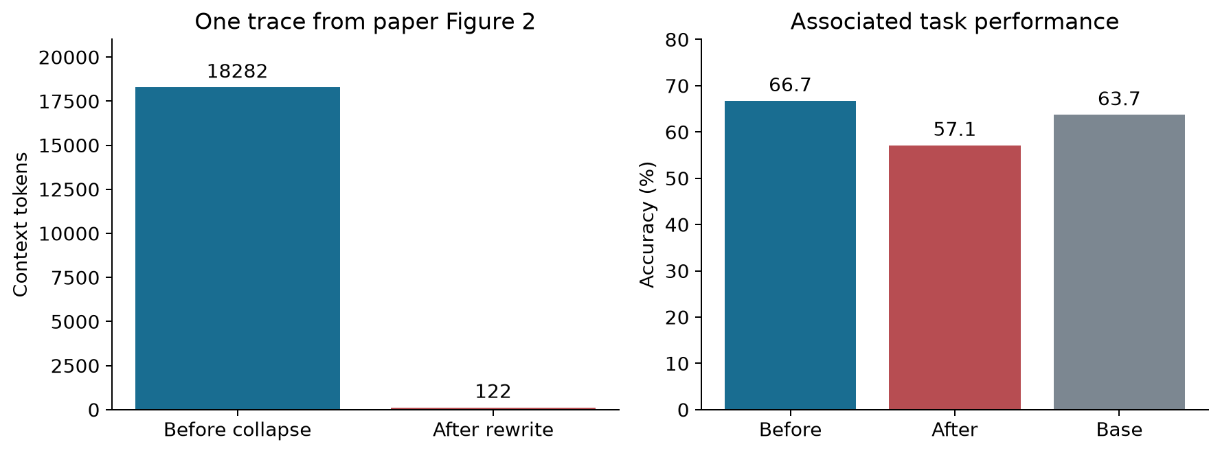
The paper illustrates a Dynamic Cheatsheet run in which a context of 18,282 tokens collapses to 122 tokens after a rewrite. The associated accuracy moves from 66.7 to 57.1, below a 63.7 base score. This supports the diagnosis that rewriting can be destructive. It does not estimate the frequency of collapse across all tasks, models and summarization prompts, nor isolate every causal factor behind that accuracy change.

3.3 A retention model for the design intuition

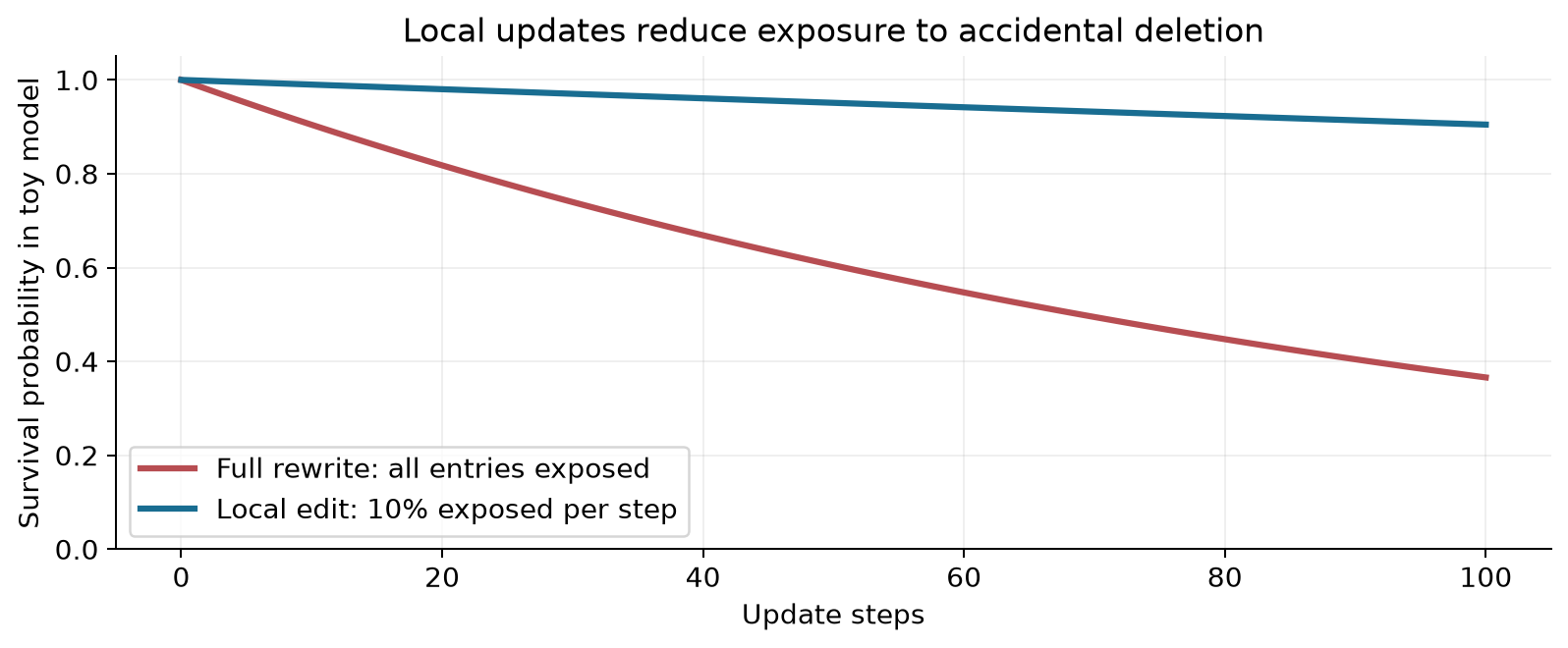
Suppose an old useful entry has probability $q$ of surviving each complete rewrite, independently across updates. Its probability of surviving $T$ rewrites is the product of those probabilities:

$$\Pr(\text{survive }T\text{ full rewrites}) =\prod_{t=1}^{T}q=q^T. \tag{3}$$

Now suppose a localized update exposes only a fraction $a$ of entries to potential editing. A particular entry is either untouched, with probability $1-a$, or touched and preserved, with probability $aq$. Its one-step survival probability is $(1-a)+aq$. Repeating the same idealized argument gives

$$\Pr(\text{survive }T\text{ local edits}) =\left[1-a(1-q)\right]^T. \tag{4}$$

At $q=0.99$ and $T=100$, full rewriting preserves an entry with probability about 0.366. With $a=0.1$, the local-edit model gives about 0.905. These are calculations under stated assumptions, not measurements of ACE. Errors in a real system are correlated; some entries are intentionally removed; and deduplication can affect more than the newly added text. The calculation explains why reducing exposure can help, without claiming a retention theorem for the deployed framework.

The same logic exposes the design’s other side. A mistaken rule also survives more easily when old content is protected. Retention and correction must be designed together. A system that only appends can preserve experience while becoming progressively harder to trust.

4. From a trajectory to a small, durable update

4.1 Three roles solve different compression problems

The Generator attempts the task using the current playbook. Its trajectory provides a record of what was tried, which observations arrived and where the process failed or succeeded. The Reflector extracts a diagnosis from that record. The Curator decides what is new relative to the existing playbook and expresses an incremental update. The final merge is lightweight deterministic logic rather than another request to rewrite the entire context.

Separating the roles makes the information boundary explicit. Reflection asks what this episode teaches; curation asks whether the collection already contains that lesson. Combining these questions in one unconstrained rewrite encourages both redundancy and accidental deletion. On the other hand, three roles mean additional calls and more opportunities for one generated interpretation to reinforce another. Role separation is organization, not independent verification.

The main experiments use the same non-thinking DeepSeek-V3.1 model for all three roles. This controls a simple alternative explanation in which a much stronger teacher supplies new knowledge to a weaker Generator. It does not eliminate correlated errors between the roles. The appendix varies the Reflector separately, which provides a more direct test of that component’s quality.

4.2 Algorithm 1: an explanatory ACE update cycle

This numbered pseudocode summarizes the paper’s method. Feedback availability and the number of refinement rounds belong to the chosen experimental setting; the pseudocode does not invent a guarantee that every update is beneficial.

Algorithm 1: One context-adaptation step
1. Read task x and the current playbook P.
2. Generator attempts x using applicable entries in P.
3. Preserve the trajectory and the available outcome feedback.
4. Reflector diagnoses errors, successes and reusable lessons.
5. Optionally refine the reflection within the allowed round budget.
6. Curator compares the lessons with P and emits local additions.
7. Deterministic merge assigns IDs and incorporates the delta.
8. Update available helpful/harmful entry metadata.
9. Deduplicate or refine entries at the configured trigger.
10. Return the updated playbook for subsequent tasks.

The trajectory in step 3 is important even when the answer is correct. An agent may succeed through unnecessary retries or a brittle shortcut. A reflection can identify a reusable procedure or a misleading rule that happened not to cause failure. However, a convincing explanation after the fact is still a hypothesis about what mattered. The paper’s helpful/harmful metadata is useful bookkeeping, not a causal estimate of each entry’s contribution.

4.3 The entry is the unit of preservation

The playbook organizes material into entries with stable identifiers, text and helpful/harmful counters. Stable identity lets later feedback refer to a particular lesson rather than a moving paragraph in a monolithic prompt. It also allows an update to leave unrelated entries unchanged.

For a conceptual representation, write

$$P_t=\{(i,c_i,h_i,b_i)\}_{i\in I_t}, \tag{5}$$

where $i$ is an identifier, $c_i$ the content, $h_i$ a helpful count and $b_i$ a harmful count. This notation is a reading aid. It does not specify an exact database schema or claim that counters alone decide every refinement action. In particular, the AppWorld and FiNER Curator prompt examples list ADD operations; the wider grow-and-refine description also discusses deduplication and metadata-driven management. These should not be conflated into an undocumented general edit language.

4.4 Algorithm 2: the merge contract and its boundary

A deterministic merger removes the risk of an LLM silently paraphrasing every old entry during an append. It cannot determine whether a new rule is true merely by checking its structure. The following is a conceptual contract for explaining that distinction. Duplicate-event protection and version checks are proposed operational safeguards, not experimentally established features of the paper.

Algorithm 2: A conservative delta-merge contract
1. Receive a delta and the playbook version it was based on.
2. Check that each proposed addition has a section and content.
3. Assign a fresh identifier to each accepted new entry.
4. Preserve all unrelated existing entries byte for byte.
5. Apply entry-feedback events to their referenced identifiers.
6. Record which update produced the new version.
7. Run the separately specified redundancy/refinement policy.
8. Return the next version and a record of changed entry IDs.

Why make step 7 separate? Structural merging and semantic consolidation have different failure modes. An append can preserve old text exactly. A semantic merge may discover that two sentences say the same thing, but it may also erase a negation, a version constraint or an exception. Treating deduplication as a cheap formatting step hides this risk.

The paper suggests semantic similarity for detecting redundant entries, with refinement either after an update or when the context reaches a limit. An aggressive threshold reduces duplicated advice but can fuse distinct procedures. A permissive threshold protects distinctions while allowing clutter. Appendix A.6 tests thresholds of 50%, 70% and 90%; FiNER accuracy is 77.0, 73.9 and 78.6. All exceed the 70.7 base, but the 4.7-point spread between two settings is large enough that I would avoid describing the choice as irrelevant.

4.5 Parallel additions are simpler than parallel corrections

Localized deltas can be batched and merged. If two tasks add independently identified entries, taking the union is straightforward. If they update the same counter or offer conflicting rules about the same API version, order and interpretation matter. The paper’s broad scalability argument does not by itself specify a conflict-resolution protocol.

For disjoint additions $\Delta_a$ and $\Delta_b$ with distinct IDs, a set-union model satisfies

$$(P\cup\Delta_a)\cup\Delta_b =(P\cup\Delta_b)\cup\Delta_a. \tag{6}$$

This commutativity follows from set union, not from a language model understanding contradictions. If two deltas replace the same content, the identity no longer describes the operation. If the same feedback event is retried twice, adding its counter increment twice also changes the result. Versioned updates and event identity would therefore be useful additions for a production system, especially when experience is collected asynchronously.

4.6 Growth requires an explicit capacity policy

A long context window postpones capacity pressure but does not abolish it. The paper’s FiNER pruning-trigger experiment reports 78.6, 78.4 and 78.3 accuracy at 10K, 50K and 100K tokens. This is evidence that the tested task did not require a finely chosen large threshold. It is not evidence that every task can use a 10K playbook or that tokens above 10K are always redundant.

A more informative question is which facts are removed first. Frequently useful general rules, rare critical exceptions and stale implementation details have different values. Counting mentions favors common cases. A robust refinement policy should preserve the conditions that make an exception necessary, and should allow a once-useful rule to expire when its environment changes.

5. Evaluation: keep the information timeline intact

5.1 Algorithm 3: score before updating

The paper’s online protocol predicts before adapting on the current sample. The following explanatory pseudocode makes that timing visible. The optional warm-start phase must be reported separately because it changes the initial state.

Algorithm 3: Sequential online evaluation
1. Choose the task order before comparing methods.
2. Set P to an empty or explicitly documented warm-start playbook.
3. For each task x_t in that fixed order:
4.     Freeze the current P while producing prediction y_hat_t.
5.     Score that prediction before changing P.
6.     Reveal only the feedback allowed in this setting.
7.     Apply one permitted adaptation step to obtain the next P.
8. Report the average of the original predictions and total cost.
9. Retain the initial state, task order and feedback policy.

Evaluating the final playbook on the same stream after it has learned from all labels would answer a different question. Likewise, an online method that starts with offline experience should not be described as learning entirely from scratch. ACE’s Table 3 reports 56.1 for online adaptation without offline warm-up and 59.5 with it. The latter matches the main Table 1 online result. The 3.4-point gap is an empirical reminder that the starting state is part of the method.

5.2 AppWorld is not one undifferentiated accuracy

AppWorld reports Task Goal Completion (TGC) and Scenario Goal Completion (SGC), each on normal and challenge splits. The main average is the mean of four reported quantities. They describe related but different levels of success; averaging them is a summary, not a replacement for the individual columns.

For the displayed ACE offline-with-labels row,

$$\bar s=\frac{76.2+64.3+57.3+39.6}{4} =59.35\approx59.4. \tag{7}$$

The base row is 42.4 after rounding, so the displayed-row gain is 17.0 percentage points. A relative gain would instead divide the difference by the base score:

$$\text{relative gain}\approx \frac{59.4-42.4}{42.4}=0.401. \tag{8}$$

These are different quantities. I use percentage points for subtractions of reported percentage scores and reserve relative percentages for ratios with an explicit denominator. That avoids turning a result into a larger or smaller claim merely through notation.

5.3 Labels and metrics differ across domains

FiNER labels financial entities using 139 fine-grained XBRL categories; Formula asks financial numerical questions. The main paper reports exact-answer accuracy for these tasks and for the appendix’s DDXPlus medical benchmark. BIRD-SQL uses GPT-4o-mini as an LLM judge in the reported setup. Its score should therefore not be casually renamed SQL execution accuracy.

The distinction matters for reflection. An incorrect fine-grained label may produce little useful signal without a reference label. An interactive task may expose a concrete failure before its final answer. A numerical answer can have an internal consistency check without establishing every financial assumption. The available evidence determines what the Reflector can plausibly learn.

None of the reported benchmarks is a measurement of indefinite, unattended self-improvement. They test bounded tasks, specific splits and particular update procedures. Generalizing to a changing production workload requires additional evidence about drift, contradictory experience and recovery after mistaken updates.

6. What the reported results support

6.1 AppWorld: a substantial gain with uneven distribution

The following values are transcribed from Table 1, with the warm-start condition for the last row clarified using Table 3. GT denotes ground-truth feedback during adaptation. The normal and challenge columns each contain TGC followed by SGC.

Method	Normal TGC / SGC	Challenge TGC / SGC	Mean
Base ReAct	63.7 / 42.9	41.5 / 21.6	42.4
Offline ICL, GT	64.3 / 46.4	46.0 / 27.3	46.0
Offline GEPA, GT	64.9 / 44.6	46.0 / 30.2	46.4
Offline ACE, GT	76.2 / 64.3	57.3 / 39.6	59.4
Offline ACE, no GT	75.0 / 64.3	54.4 / 35.2	57.2
Online DC, no GT	65.5 / 58.9	52.3 / 30.8	51.9
Online ACE, warm start, no GT	69.6 / 53.6	66.0 / 48.9	59.5

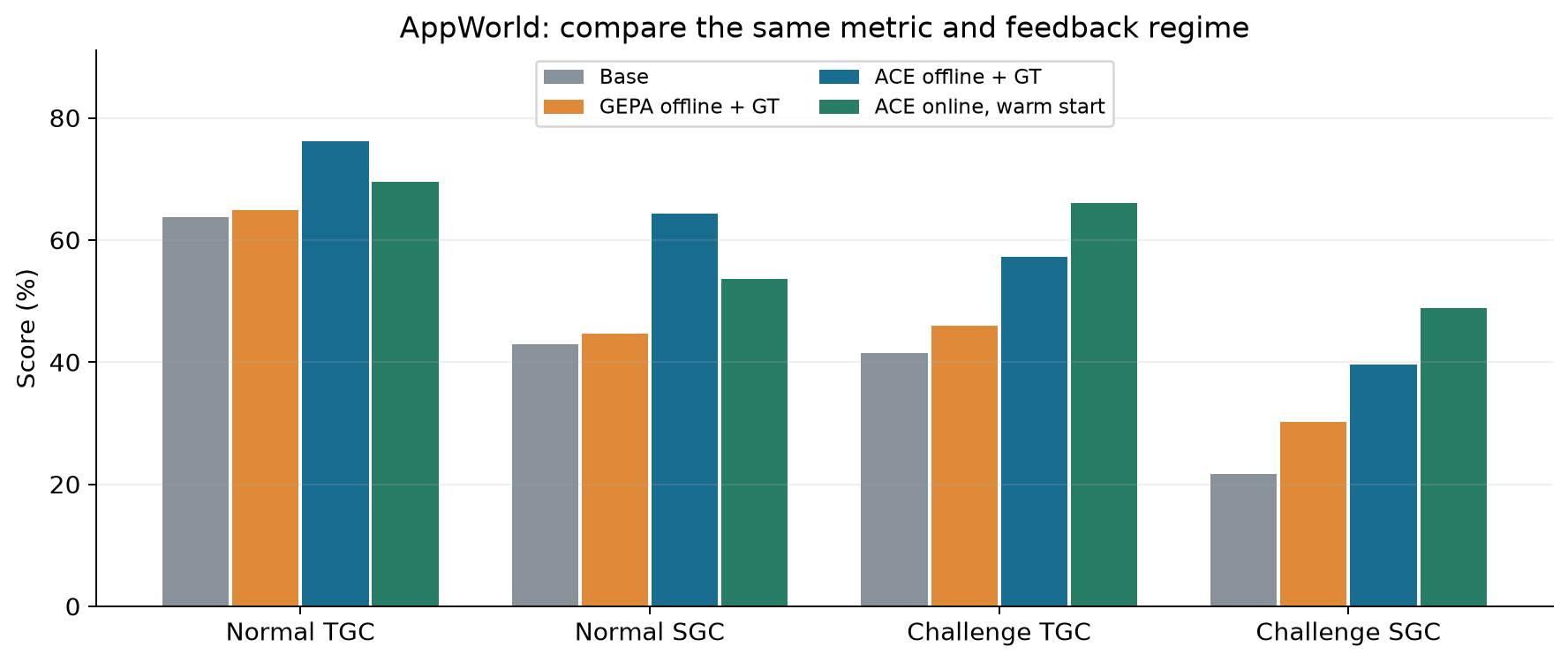
The gain over a static prompt is broad, including the harder split. However, the online row is not uniformly better than offline ACE: it improves challenge scores while reducing normal scores. That is consistent with an evolving playbook changing which tasks it serves best. A single aggregate cannot show that distribution.

There is also a reporting discrepancy worth keeping visible. The paragraph below Table 1 describes gains of 12.3 and 11.9 over ICL and GEPA. Subtracting the displayed averages instead gives 13.4 and 13.0 percentage points for offline ACE with GT. The no-GT row does not recover those stated differences either. Without a matching aggregation definition, I use the table values rather than silently reconciling them. This observation does not invalidate the direction of the result, but it limits precision when repeating the headline.

The September 2025 leaderboard comparison is historical context. ACE’s 59.4 is near IBM CUGA’s reported 60.3, not numerically identical. The authors explicitly caution that CUGA has a different system design and is not a controlled baseline. It would be misleading to turn this snapshot into a current leaderboard claim or a controlled comparison of model parameter efficiency.

6.2 Financial tasks expose the feedback boundary

ACE setting	FiNER	Formula	Average
Base model	70.7	67.5	69.1
Offline, GT	78.3	85.5	81.9
Offline, no GT	71.1	83.0	77.1
Online, GT	76.7	76.5	76.6
Online, no GT	67.3	78.5	72.9

The online no-GT average exceeds the base average, yet FiNER falls by 3.4 points. Formula gains 11.0 points. Aggregation therefore hides a meaningful failure mode: some knowledge can be usefully refined without labels, while a finely differentiated classification system can reinforce its own mistakes. The correct takeaway is conditional adaptation, not reliable label-free improvement everywhere.

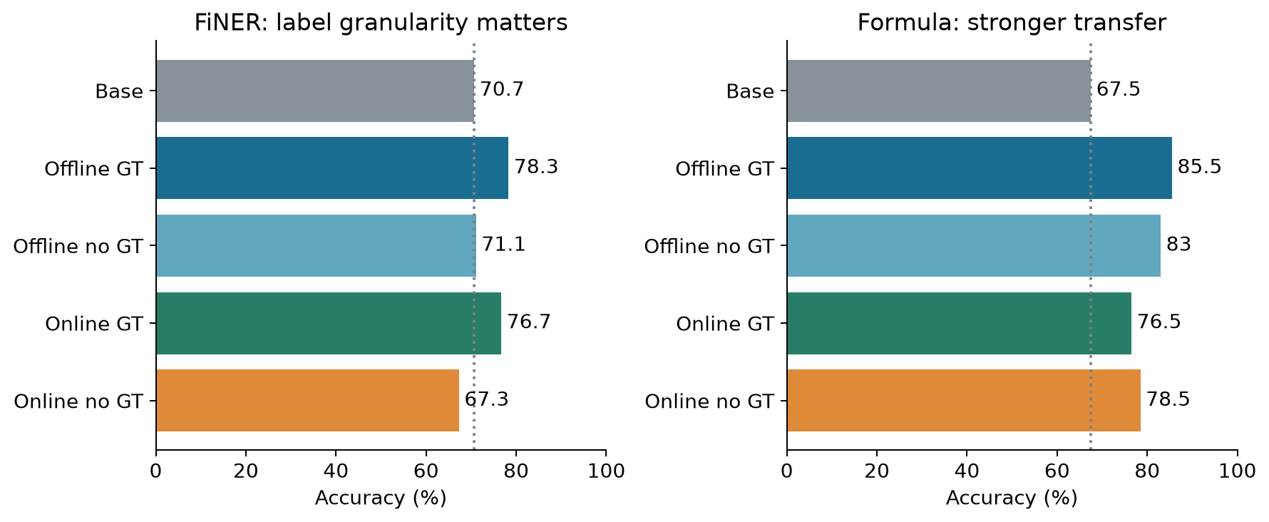
Offline ACE with labels reaches 81.9 on the two-task average, versus 72.5 for GEPA and 70.9 for MIPROv2. Those gaps should not be conflated with the online comparison. Likewise, the Formula value 76.5 shown for online ACE with GT is different from the best offline value 85.5. Mixing them across figures and tables would create a nonexistent configuration.

6.3 Which components seem to matter?

Table 3 presents a nested offline ablation: removing both the Reflector and multiple epochs gives 55.1; retaining the Reflector but using one epoch gives 56.8; the full setting gives 59.4. The successive differences are 1.7 and 2.6 points. They support the usefulness of both additions in that sequence, but do not form a complete factorial experiment. We cannot infer an interaction-free, universal contribution for each component.

Appendix Table 18 more directly compares incremental updates with a version lacking them. On the normal-split average, the base is 53.3, ACE without incremental updates is 56.9, and ACE with them is 70.3. The difference between the ACE variants is 13.4 points. The table’s TGC difference is 8.9 points and its SGC difference 17.9 points. Appendix C expresses corresponding losses as relative percentages, so readers should keep the denominator explicit.

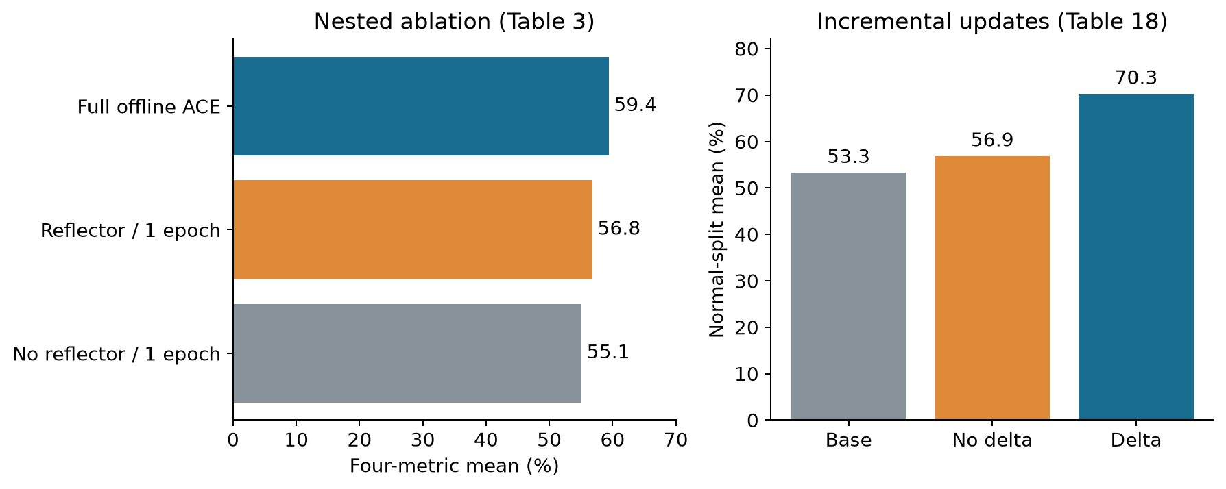
The incremental-update ablation is stronger evidence for the retention mechanism than the single collapse trace alone. It still leaves practical questions about how an equally budgeted, carefully constrained full-rewrite baseline would behave. A weaker baseline can be easier to beat, so the most useful follow-up would hold feedback, model calls, context capacity and task order fixed while varying the update representation.

6.4 Additional models strengthen transfer, not universality

With GPT-OSS-120B, AppWorld’s base average is 34.6; offline ACE with GT reaches 40.5, and the reported online ACE row reaches 42.2. With GPT-5.1, the appendix reports normal-split averages, so they are not directly comparable to those four-column means: the base is 54.2 and online ACE is 65.8. FiNER on Llama-3.3-70B improves from 62.5 to 64.9 in the offline-with-labels setting, a smaller gain than the headline DeepSeek result.

Beyond finance, DDXPlus improves from 75.2 to 90.2, while BIRD-SQL improves from 47.8 to 52.9 overall. On BIRD’s moderate and challenging subsets, GEPA scores higher than ACE. The overall average is not the unweighted average of the three displayed subset scores; it reflects the benchmark’s overall evaluation. Replacing it with an arbitrary three-way mean would change the reported quantity.

These results make the method more credible as a general pattern. They do not show every model benefits equally or every subtask prefers ACE. Some additional comparisons use different validation resources, and confidence intervals over multiple adaptation trajectories would help separate robust improvements from particular run choices.

7. Cost: distinguish writing memory from using memory

7.1 Why small deltas can save generated tokens

Suppose a playbook starts at $L_0$ tokens and gains $a$ tokens per update. A full rewrite emits the entire current playbook at each of $T$ steps. In a simple model, the total emitted context text is

$$W_{\mathrm{full}}=\sum_{t=1}^{T}(L_0+at) =TL_0+\frac{aT(T+1)}{2}. \tag{9}$$

The first equality counts each rewrite; the second uses the arithmetic-series sum. If a delta contains $d$ tokens per step, emitting only changes costs

$$W_{\mathrm{delta}}=Td. \tag{10}$$

This explains a possible linear-versus-quadratic difference in context-writing output, under a growing-playbook model. It is not a total-runtime theorem. A Curator that reads the entire playbook still incurs increasing input cost, and the Generator may repeatedly receive the accumulated context during a multi-step task. Reflection outputs, validation calls and deduplication are also omitted from this toy calculation.

For illustration, at $L_0=1{,}000$, $a=d=100$ and $T=100$, full rewrites emit 605,000 tokens while deltas emit 10,000. The 60.5-fold ratio is arithmetic for this hypothetical workload; it is not a measured ACE speedup. The point is to identify which term the architecture removes and which terms remain.

7.2 The headline adaptation measurements

Table 4 reports AppWorld offline adaptation latency of 53,898 seconds for GEPA and 9,517 for ACE, with rollout counts of 1,434 and 357. The latency reduction is

$$1-\frac{9{,}517}{53{,}898}=0.8234, \tag{11}$$

or about 82.3%. The corresponding speed ratio is about 5.66, while the rollout reduction is about 75.1%. For online FiNER, Dynamic Cheatsheet versus ACE is 65,104 versus 5,503 seconds and 17.7 versus 2.9 dollars. Those imply approximately 91.5% lower adaptation latency and 83.6% lower reported cost in that setting.

These are adaptation measurements under the paper’s configurations. They do not mean that each future request is 5.66 times faster, nor that dollar savings remain unchanged on another provider. Model prices, caching and the number of repeated uses of the resulting playbook all affect the application-level outcome.

7.3 The appendix complicates the rollout story

Appendix A.3 gives a separate detailed accounting, using one ACE epoch and one reflection-refinement round. There GEPA uses 204,076,096 input tokens and 1,870,188 output tokens during adaptation. ACE uses 39,250,925 and 307,128, reductions of 80.8% and 83.6%.

But its total rollout counts are 2,075 for ACE versus 1,455 for GEPA, an increase of 42.6%, because the accounting lists calls across Generator, Reflector and Curator. These numbers cannot be substituted for Table 4’s counts. The configurations and counting boundaries must be reported alongside the metric; the paper does not provide a single conversion that makes both tables one universal rollout advantage.

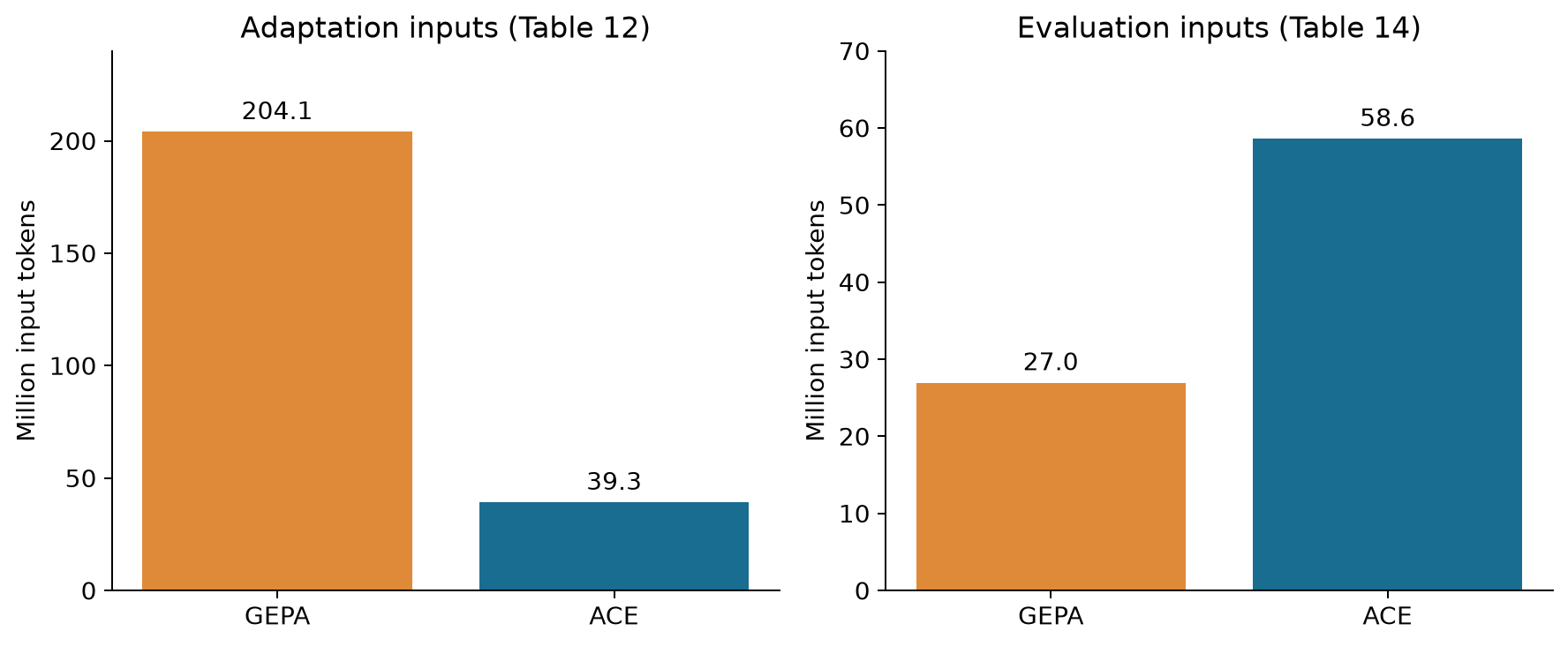
At evaluation, Table 14 reports 58,623,267 ACE input tokens versus 26,960,675 for GEPA across the same 160 queries: an increase of 117.4%. Output tokens increase by 7.6%, while rollouts decrease by 4.7%. This is an instructive trade: investing in a more detailed playbook can improve quality while increasing the raw context that the model must consume.

7.4 Cache savings need their own denominator

Let uncached input cost per token be $p$, cached cost be $\rho p$, total input volume be $N$, and the cached fraction be $c$. Splitting the input into cached and uncached parts gives

$$K=pN(1-c)+\rho pNc =pN[1-c+\rho c]. \tag{12}$$

Relative to serving the same inputs entirely uncached, the saving is

$$1-\frac{K}{pN}=c(1-\rho). \tag{13}$$

At $c=0.918$ and $\rho=0.1$, the saving is 0.8262, or 82.62%. This explains the paper’s approximately 91.8% cached input and 82.6% input-cost reduction in its GPT-5.1 caching analysis. It is not evidence of an 82.6% total-cost advantage over GEPA. The denominator excludes output cost and uses the same ACE context volume, not a competing system’s smaller prompt.

Caching also depends on request structure. Stable shared prefixes can be reused; frequently changing text near the beginning can reduce reuse farther into the prompt. An append-oriented playbook may make prefix reuse easier, but actual cache eligibility, routing and expiration determine the benefit. Billing discounts do not prove the absence of KV-memory pressure or long-context decode cost.

7.5 More reflection can also be wasted work

Table 19 reports normal-split averages of 61.3, 65.8, 67.6 and 65.2 for one, three, five and ten reflection rounds. More rounds do not monotonically improve the result. A plausible mechanism is that additional reflection first extracts missed lessons and later produces redundant or noisy advice. The experiment supports a finite useful budget; it does not isolate that mechanism conclusively.

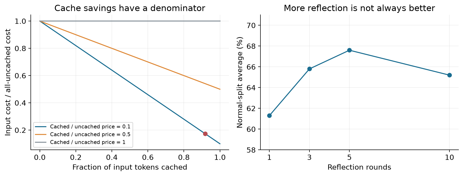
A sensible deployment decision would compare quality against total adaptation cost, total serving cost and tail latency. For a playbook reused many times, inference overhead can eventually dominate the one-time adaptation saving. For a short-lived task family, the opposite may be true. The paper supplies useful components of that calculation but does not establish one universal economic break-even point.

8. Limitations and failure boundaries

8.1 Better preservation also preserves wrong advice

Appendix Table 17 injects a harmful reflection every $X$ adaptation steps on FiNER. Accuracy is 66.7 when every step is corrupted, below the base’s 70.7. At frequencies of one in five, ten, twenty-five, fifty and one hundred, scores are 76.1, 77.0, 77.8, 78.2 and 78.2; without harmful reflection the score is 78.3.

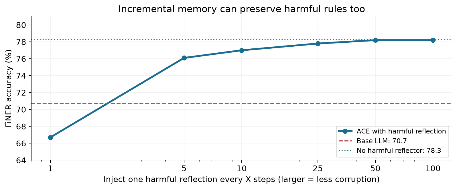
This is stronger evidence than merely warning that reflection might be wrong. Yet the tested corruption schedule is not a complete threat model. A rare, highly plausible rule applied across many future tasks could have a different effect from the injected feedback. Long-lived poisoning, targeted contradictions and environment changes remain useful stress tests.

8.2 Useful detail can become brittle over-specificity

An operational rule may be correct for one environment and wrong after an API change. An entry can also contain a task-specific constant disguised as a general strategy. The prompt examples in the appendix illustrate how concrete domain advice can become; that concreteness is useful only if the scope is preserved.

The alternative of a very short instruction has its own cost: it may lack the detail needed to prevent repeat failures. The right boundary is conditional specificity. A rule should state what must be true for it to apply, which observation supports it, and which parts are examples rather than universal constants. These are recommended design properties, not guarantees established by the paper’s aggregate benchmark gains.

8.3 Semantic similarity is not semantic equivalence

Two entries can mention the same objects while prescribing opposite actions. A negation, a version number or a unit can be the most important part of the sentence and contribute little to an embedding’s overall similarity. Merging on similarity alone therefore risks erasing precisely the exception that made a rule useful.

The paper’s threshold experiment is reassuring within its measured range, but a high FiNER score is not a proof of contradiction-safe consolidation. A stronger test would deliberately construct near-duplicate rules whose applicability differs, then measure whether the refined playbook keeps the distinction. This tests the retention mechanism more directly than checking only average task accuracy.

8.4 Context access and model competence remain bottlenecks

Preserving an entry does not ensure that the Generator notices or follows it. As the playbook grows, relevant rules compete with other context. Rules can also require capabilities the model does not have. A detailed instruction cannot guarantee correct multi-step arithmetic or perfect interpretation of a complicated API.

This suggests three separate failure categories: a useful lesson was never learned; it was learned but later lost; or it remained present but was not used correctly. ACE primarily improves the second category and organizes the first. A retrieval or routing layer may help the third, but brings its own missed-retrieval and selection errors. Evaluations should distinguish these cases rather than attributing every gain or failure to memory size.

8.5 The evidence is finite and configuration-dependent

The paper covers several models and domains, yet does not demonstrate unlimited continual learning. The available result tables also do not establish confidence intervals over all possible task orders or adaptation seeds. Reported point estimates can motivate a design without defining the uncertainty of every difference.

Other qualifications matter: some additional tasks use different validation resources for baselines; online results can include a warm start; and BIRD uses an LLM judge. These are not reasons to discard the study. They are reasons to carry the experimental setup with the result when deciding whether it transfers to a new application.

9. Independent critical analysis: what would make the memory trustworthy?

9.1 Entry counters are observations, not causal credit

Suppose the Generator cites entry A on an easy question and succeeds, then cites entry B on a difficult question and fails. Incrementing A’s helpful count and B’s harmful count may reward task difficulty rather than rule quality. The Generator’s choice of entries is itself correlated with what it finds challenging.

A descriptive ratio such as

$$\widehat u_i=\frac{h_i}{h_i+b_i} \tag{14}$$

is undefined without observations and otherwise reflects selected usage, not a randomized intervention. Adding smoothing avoids division by zero but does not fix selection bias. A useful improvement would occasionally compare matched tasks with and without an entry, while keeping the rest of the context fixed. Such ablations cost extra calls; that cost belongs in any claim about cheaper learning.

There is also delayed credit. A rule may prevent an error several steps before the final answer, while the final reflection notices only the last successful action. Recording the evidence and applicability of an entry may be more informative than a single lifetime counter, especially when the environment changes.

9.2 A simple acceptance threshold makes asymmetry visible

Consider a proposed rule that is correct with probability $q$. If correct, it produces expected downstream gain $g$; if wrong, it causes expected harm $h$. Ignoring interactions and assuming these quantities summarize future uses, its expected net value is

$$V=qg-(1-q)h. \tag{15}$$

To accept only positive expected value, rearrange $qg>h-qh$ into

$$q>\frac{h}{g+h}. \tag{16}$$

This is a decision-theory illustration, not ACE’s published acceptance rule. It shows why one confidence threshold is inadequate when errors have different consequences. If a false rule is cheap to notice and undo, moderate confidence may suffice. If it silently contaminates many future tasks, $h$ grows and the required confidence approaches one. The harmful-reflector experiment is evidence that this asymmetry deserves measurement.

A practical extension would place weakly supported rules in a provisional state, require more evidence for broadly applicable rules, and retain a route to withdraw them. That need not imply another powerful model judges everything. Evidence from repeated independent outcomes may be more useful than several correlated reflections on the same trajectory.

9.3 Retention needs forgetting and rollback

Incremental updates solve accidental rewriting loss, but indefinite retention can preserve stale rules. A useful state should include when and where an entry was observed, not just how often it was once helpful. A rule supported under an old API may deserve reevaluation even with a high lifetime score.

A controlled rollback is also different from semantic deletion. Removing a rule from the active playbook can stop future use, but it does not erase copies in logs, cached contexts or earlier versions. Claims about selective forgetting should specify the object being changed. For this paper, readable external context makes editing and inspection easier; it does not demonstrate complete erasure throughout an application.

9.4 Algorithm 4: a sharper experiment for the central claim

I would test the claim that incremental context management preserves useful experience under a fixed information and computation budget. The following is a proposed evaluation, not an experiment performed for this review.

Algorithm 4: Budget-matched retention evaluation proposal
1. Fix model, training tasks, feedback sources and total token budget.
2. Compare full rewrite, append-only and incremental-refinement states.
3. Give each method the same maximum context capacity.
4. Repeat adaptation over several fixed task orders.
5. Insert rare exceptions, contradictory evidence and a domain shift.
6. Score before updates; keep an independent frozen hold-out set.
7. Track entry survival, correct retrieval, usage and task success.
8. Report quality, input/output tokens, latency and recovery time.
9. Release the evaluation protocol and uncertainty estimates.

The append-only baseline is particularly informative. If it matches ACE under the same capacity, the benefit may come mainly from preservation. If refinement wins after the context saturates, the management policy adds value beyond append-only storage. A full-rewrite method constrained to preserve protected entries would further test whether structure or prompting explains the gap.

9.5 Where ACE sits in harness self-improvement

ACE changes the agent’s accumulated instructions and knowledge. A harness can additionally change tool interfaces, execution control, testing strategy and the procedure that decides future updates. Improving a playbook is therefore one layer of a larger self-improving system.

The natural next research question is whether the update procedure itself should evolve. That introduces a second feedback loop: an outer process changes how experience is interpreted, while an inner process changes what the agent remembers. Such a system needs separate evaluation of the current playbook and the policy producing it. ACE provides a concrete inner-loop design and valuable failure cases, but its results should not be presented as evidence that arbitrary self-modification is already reliable.

10. Conclusion

ACE’s strongest idea is to treat accumulated context as a collection of durable, individually addressable lessons. Separating generation, reflection and curation makes the update understandable; emitting local deltas protects unrelated knowledge from repeated rewriting. The AppWorld and finance results, incremental-update ablation and additional models support that design under the reported conditions.

The qualification is equally useful. Retention can preserve errors, label-free feedback can degrade classification, and longer playbooks can increase evaluation input cost. The next advance should measure the whole learning loop: what was learned, what survived, what remained applicable, what the Generator actually used, and what the full system paid for it.

For a reader interested in self-evolving harnesses, ACE is a good starting point precisely because its update object is concrete. It makes the promise of accumulating experience testable, while leaving room to ask when a memory should be trusted, corrected or forgotten.

References and figure provenance

1. Zhang et al., Agentic Context Engineering: Evolving Contexts for Self-Improving Language Models, arXiv:2510.04618v3, ICLR 2026. The main source for all reported experiments: Tables 1-4 and Appendix Tables 5-21; full prompt examples in Appendix F.
2. ACE author project and official resource, provided as entry points for readers.
3. Figure 1 is an original structural summary. Figure 2 redraws the paper’s illustrative collapse example. Figure 3 is a stated toy calculation. Figures 4-7 and 9 redraw reported table values; Figure 8 combines an explanatory cost identity with Table 19. All equations and numbered pseudocode in this review are explanatory formulations or explicitly marked proposals, rather than verbatim paper algorithms.
4. Terminology: GT means ground-truth feedback during adaptation; “online” means predict before update; percentage-point differences and relative reductions use the denominators stated in the text. No reported result is presented as a new measurement by this review.