FlashInfer: Making Attention Fit the Serving Workload

Review date: September 27, 2026
Author: Zhongzhu Zhou
Paper reviewed: FlashInfer: Efficient and Customizable Attention Engine for LLM Inference Serving
Paper authors: Zihao Ye, Lequn Chen, Ruihang Lai, Wuwei Lin, Yineng Zhang, Stephanie Wang, Tianqi Chen, Baris Kasikci, Vinod Grover, Arvind Krishnamurthy, Luis Ceze
Version: arXiv:2501.01005v2, April 21, 2025
Sources: Versioned paper, project, official code resource

1. The question I wanted this paper to answer

An attention kernel can be excellent on one contiguous tensor and still be a poor serving component. Real requests arrive with different prompt lengths, finish at different times, share some prefixes, and refer to KV data scattered across physical pages. The next decoding step changes this workload again. A useful engine must accommodate that variation without paying a large scheduling or launch cost at every layer.

I read FlashInfer as a study of where to place the boundaries between mathematical computation, memory representation, and runtime scheduling. Its three central choices reinforce each other: represent access patterns with block-sparse views; make attention outputs composable; and put changing work assignments in data that a fixed GPU program can consume. JIT specialization then handles choices that should remain static during execution.

The result is more interesting than a single fast attention formula. It is a way to expose reuse and parallelism that the serving framework already knows about. A page table tells us where tokens live. A shared-prefix relation tells us which queries can reuse the same data. Sequence lengths tell us how much work each request needs. FlashInfer turns those facts into a kernel execution plan.

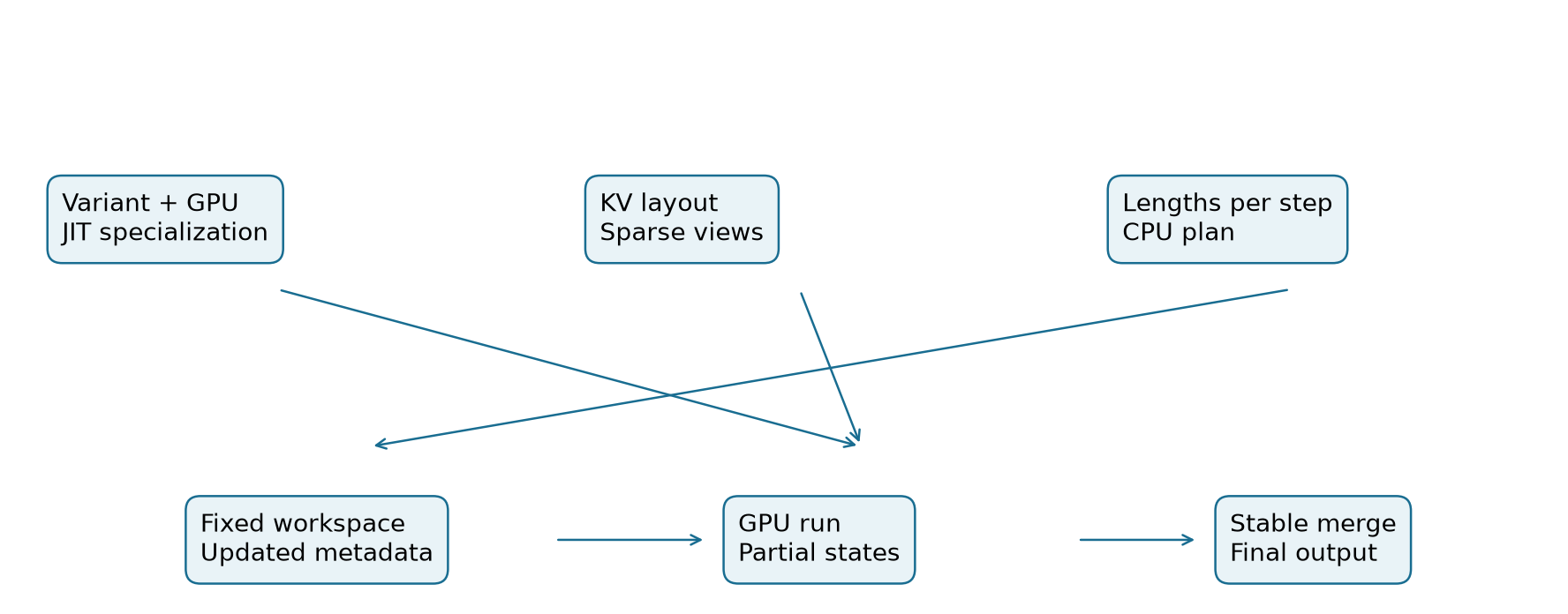
The evidence is conditional. The main experiment reports substantial inter-token latency improvements in SGLang, while the appendix includes near-neutral scheduler effects for short workloads and a bf16 latency regression in vLLM. I will keep these different scopes separate. All measured numbers below are reported by the paper; the toy examples and derived ratios are my explanations, not new serving measurements.

2. Prerequisites: what changes between prefill and decoding?

2.1 The same operator, different shapes

For one query head, let the query, key, and value matrices have shapes $Q\in\mathbb{R}^{L_q\times d}$ and $K,V\in\mathbb{R}^{L_k\times d}$. With a validity mask $M$, standard attention is

$$S=\frac{QK^\top}{\sqrt d}+M,\qquad O=\operatorname{softmax}(S)V. \tag{1}$$

The mask contributes zero to allowed scores and negative infinity to forbidden scores. During prompt prefill, $L_q$ can be large; during ordinary autoregressive decoding, each request contributes just one new query. In both cases a query can read many historical keys. A tensor-core configuration that efficiently processes hundreds of query rows may waste most of its work on a one-row decoding request.

2.2 A first-order operational-intensity calculation

Ignoring masking, softmax, and repeated tile loads, the two matrix products require about $4L_qL_kd$ floating-point operations. Reading the input tensors and writing the output once costs approximately $2bd(L_q+L_k)$ bytes, where $b$ is bytes per scalar. Thus an idealized intensity is

$$I_{\mathrm{ideal}} =\frac{4L_qL_kd}{2bd(L_q+L_k)} =\frac{2}{b}\frac{L_qL_k}{L_q+L_k}. \tag{2}$$

For $L_k\gg L_q$, this approaches $2L_q/b$. It explains the paper’s $O(L_q)$ scaling without claiming an exact hardware roofline. Real kernels add indexing, partial outputs, padding, and redundant loads. A larger batch of unrelated one-token requests adds both computation and KV traffic, so batching alone does not supply reuse of one request’s keys by another.

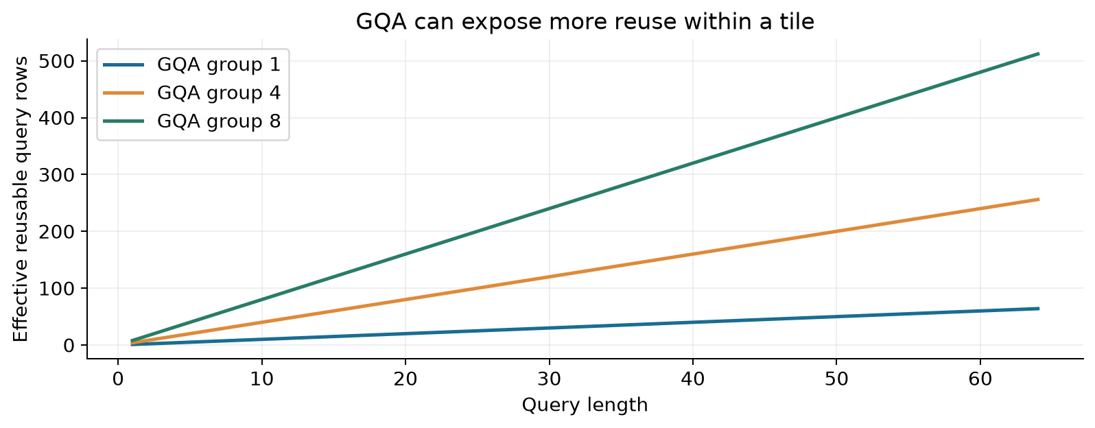
Grouped-query attention changes this opportunity. Let $g=H_q/H_{kv}$ query heads share each KV head. If a tile reuses a KV load across those heads, the effective row count becomes $gL_q$. Appendix A describes a mapping from fused row $r$ to query position and head:

$$i=\left\lfloor\frac r g\right\rfloor,\qquad h_q=g h_{kv}+(r\bmod g). \tag{3}$$

At $L_q=3,g=5$, fifteen fused rows represent three positions across five query heads. They remain fifteen distinct attention computations; fusion only changes where their shared keys are loaded. Long queries already offer substantial reuse, so the extra benefit of head fusion is most compelling for short queries.

2.3 What a CTA and a persistent kernel mean here

A cooperative thread array, or CTA, is a GPU thread block. Streaming multiprocessors execute CTAs subject to register, shared-memory, and thread limits. If one CTA owns a very long request while others finish short ones, much of the GPU can become idle even though attention work remains.

A persistent kernel launches a fixed pool of CTAs and gives each a list of work items. This decouples the number of logical attention tiles from the number of launched blocks. It does not guarantee perfect balance: the work lists, tile costs, and reduction overhead still matter. FlashInfer uses a CPU planning step to decide those lists, then lets GPU execution follow the plan.

3. Attention states: the algebra that permits decomposition

3.1 Why an output vector alone is insufficient

For one query, absorb scaling and masking into score $s_i$. For an allowed index set $A$, define its normalizer and weighted numerator:

$$Z_A=\sum_{i\in A}e^{s_i},\qquad N_A=\sum_{i\in A}e^{s_i}v_i. \tag{4}$$

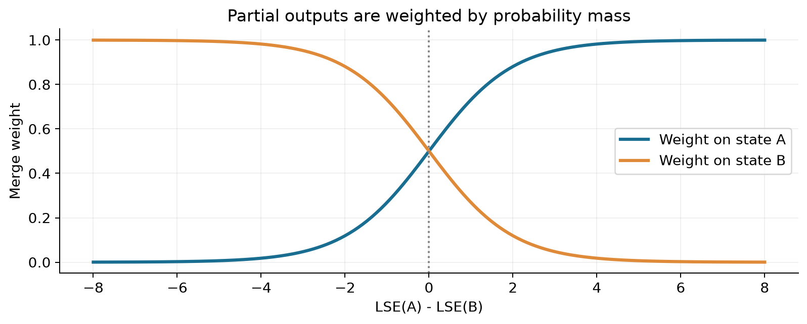
The output is $O_A=N_A/Z_A$, and its log-normalizer is $\ell_A=\log Z_A$. Knowing only $O_A$ loses how much probability mass the partition contained. Two subsets may have identical normalized outputs yet very different total mass relative to another subset.

For disjoint sets $A$ and $B$, their numerators and denominators add. Substituting $N_A=e^{\ell_A}O_A$ gives

$$O_{A\cup B} =\frac{e^{\ell_A}O_A+e^{\ell_B}O_B} {e^{\ell_A}+e^{\ell_B}}. \tag{5}$$

This is the reason FlashInfer returns an attention state $(O,\ell)$. It is enough information to combine independently computed chunks exactly in real arithmetic.

3.2 Make the merge numerically stable

Directly exponentiating a large log-normalizer is unsafe. Subtract a common maximum $m=\max(\ell_A,\ell_B)$ and define $a=e^{\ell_A-m}$, $b=e^{\ell_B-m}$. The same output becomes

$$O_{A\cup B}=\frac{aO_A+bO_B}{a+b},\qquad \ell_{A\cup B}=m+\log(a+b). \tag{6}$$

Both exponentials are at most one. This shift changes neither the ratio nor the represented normalizer. If one subset is empty, its mass is zero and the other state should pass through. If both are empty, computing negative infinity minus negative infinity is invalid; an explicit empty-state rule is necessary. That guard is a mathematical requirement of the explanation, not an assertion about undocumented behavior.

Suppose $Z_A=2,Z_B=6,O_A=1,O_B=5$ for scalar values. The correct merged output is $(2+30)/8=4$. Averaging the two outputs gives $3$, which is wrong. The difference is not a small numerical effect: separate softmax operations normalized away information that the merge must restore.

3.3 Algorithm 1: stable composition of two states

The following is explanatory pseudocode derived from Section 2.2. A valid flag avoids using an arbitrary output value for an empty partition.

1. Input states A=(OA, lA, validA), B=(OB, lB, validB).
2. If neither state is valid, return an empty state.
3. If only A is valid, return A; if only B is valid, return B.
4. Set m = max(lA, lB).
5. Set a = exp(lA - m), b = exp(lB - m).
6. Set O = (a * OA + b * OB) / (a + b).
7. Set l = m + log(a + b).
8. Return (O, l, true).

Associativity follows from addition of $(N,Z)$ before normalization. Commutativity follows for the same reason. These identities assume the partition contains each allowed key exactly once. Overlapping subsets double-count their intersection; a shared physical page may be reused by different queries, but it must not be counted twice for the same query.

Finite precision adds a second qualification. Different reduction orders can round differently even when they are algebraically equivalent. Section 3.3 uses deterministic aggregation order for identical sequence-length information and avoids nondeterministic atomic aggregation. This supports repeatability for a fixed plan; it does not establish bitwise equality between all possible partitions or GPU architectures.

3.4 One abstraction, two useful decompositions

Split-K divides a long KV sequence so several CTAs can help one query. Prefix decomposition instead divides the same query’s visible keys into shared and private regions so many queries can reuse a prefix load. Both require the same state merge, although their performance motivations differ.

This is the design choice I find most reusable. We can optimize which work happens together without changing the mathematical attention operator. The cost is additional state storage, metadata, and composition. A decomposition is worthwhile only when the parallelism or reuse it creates exceeds those costs.

4. Sparse representation without changing the attention problem

4.1 A page table is also an access pattern

FlashInfer treats the relation between query tiles and physical KV pages as a block-sparse matrix. A row identifies a group of queries; a nonzero column block identifies KV data they access. The block row size $B_r$ follows the query tile; the block column size $B_c$ follows the cache-management granularity.

This use of sparsity does not automatically mean approximating attention. A request can attend to every token in its own history while accessing only a small subset of the server’s global page pool. Conversely, if an upstream method removes relevant KV tokens, FlashInfer efficiently evaluates that restricted operator; the quality consequences belong to the sparsification method.

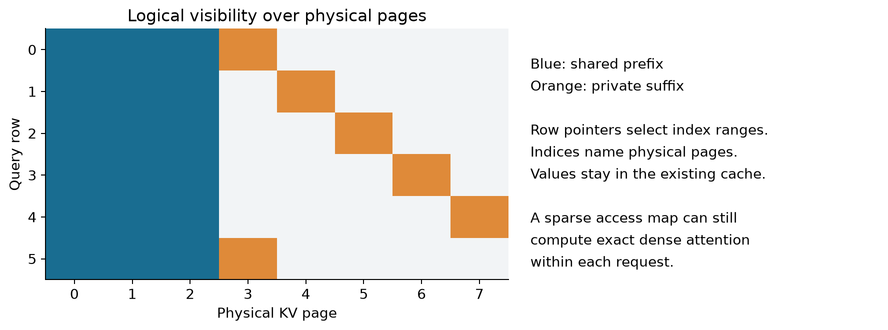
For a simple paged sequence with page size $B_c$, local token position $t$ maps to physical token position

$$p=\operatorname{indices}\!\left[\left\lfloor t/B_c\right\rfloor\right], \qquad t_{\mathrm{physical}}=pB_c+(t\bmod B_c). \tag{7}$$

For example, a request with page indices $[7,2]$ and page size four maps its logical token five to physical token nine: the second page is physical page two, with offset one. The head and feature dimensions add their own strides after this token lookup. Logical token order and physical page order are different concepts.

The row pointers delimit which page indices belong to each request. Ragged query tensors pack variable-length requests without padding all requests to the longest one. Correctness still requires per-request length information: the last physical page can contain unused slots, and causal masks must use logical positions rather than physical addresses.

4.2 Gather first, then use dense tensor operations

Tensor cores prefer regular matrix tiles, while page indices are irregular. Section 3.2 bridges these requirements by gathering scattered KV rows into contiguous shared memory. The matrix multiply can then operate on a regular tile. The feature dimension remains contiguous, helping coalesced loads even when adjacent logical tokens come from different pages.

The paper describes 128-byte asynchronous copies and distinguishes contiguous Hopper loads using TMA from arbitrary indexed gathers. A newer data-movement primitive cannot remove a mismatch in its supported address patterns. Appendix B also notes that sufficiently large sparse blocks could permit fixed-stride TMA loads inside each block; that optimization is discussed as future work in this version.

4.3 Why compose several sparse views?

A single block size trades reuse against fragmentation. Large query blocks can share one prefix load across many queries, but private suffixes do not generally have that sharing structure. Small blocks handle private regions naturally but fail to exploit common prefixes within a CTA.

Composable formats give the prefix and suffix separate views and suitable row tile sizes. The underlying KV cache need not move; new index arrays describe the decomposition. Each view produces attention states, which are then merged. This preserves unified cache management while permitting different compute layouts.

An alternative is one universal large tile with extensive masking. It simplifies representation but can spend resources on invalid rows or unshared regions. Another is permanently separating prefix and suffix storage in the serving engine. That may accelerate a narrow case but couples memory management to the attention implementation. FlashInfer’s views offer a more flexible boundary, at the expense of planning and merging.

5. Specialize the computation, not every request length

Section 3.2 describes templates built from FlashAttention-2 and FlashAttention-3 algorithms. The paper-era design targets NVIDIA architectures from Turing through Hopper. I treat those backend and version statements as historical experimental context, not a current software-support matrix.

The FA2 template has query tile choices $1,16,32,64,128$ and KV tile choices $32,64,128$. Query tile one uses CUDA cores; larger query tiles use tensor cores. Hopper FA3 templates use row tiles aligned with WGMMA requirements. These are template design choices, not a guarantee that an arbitrary application-level block size becomes an arbitrary hardware matrix instruction.

The heuristic first considers average effective query length, including head-group fusion where applicable, then selects resources subject to register and shared-memory constraints. A larger tile can reuse more data but reduce resident CTAs. If the register footprint forces spilling, the nominally more efficient tile may be slower. Average length is convenient, but a heavy-tailed batch contains information that an average does not retain.

5.1 Where customization enters

The variant interface provides query, key, value, logit, mask, and output transformations. JIT code generation inserts the variant into the optimized template along with data types, head dimensions, and other static traits. A small mathematical change therefore need not require rewriting all data movement and scheduling.

For instance, a score soft cap can be expressed as

$$\widetilde{s}=c\tanh(s/c),\qquad c>0. \tag{8}$$

The derivative is $1-\tanh^2(s/c)$, so large-magnitude scores become less sensitive to further changes. This example explains a supported transformation category; the paper’s performance tables, not this derivative, establish its measured runtime cost. A mask has a different role: it defines which scores participate at all. The ordering of score transforms and masking must preserve that distinction.

RoPE fusion is another useful example. A separate preprocessing pass writes transformed keys that an attention pass then rereads. Fusing the transformation into the load/compute path can remove intermediate traffic and a launch. It can also increase instructions and registers within attention. The net effect depends on the workload and on whether transformed keys would otherwise be reused.

5.2 An important boundary: softmax is optional

The paper also describes sigmoid attention without softmax. The template can support a different scan or reduction, but the softmax-state merge in Equation 6 should not be applied blindly. For unnormalized sigmoid weights,

$$O=\sum_i \sigma(s_i)v_i, \tag{9}$$

disjoint partial outputs add directly. They do not require the softmax log-normalizer. Customization must preserve the reduction algebra of the chosen operator. Reusing a kernel skeleton is broader than claiming all attention variants have identical mathematical states.

This boundary matters when judging extensibility. The template makes many local transformations convenient, but an operator with a different cross-token dependency or state transition may require a new scan, scheduling scheme, or template. Forward attention support in the paper does not establish customizable backward support or universal coverage of sequence models.

6. Scheduling an irregular batch

6.1 Split enough work to fill the GPU

Let request $i$ have lengths $L_{q,i},L_{k,i}$ and query tile size $T_q$. A useful proxy for total KV work across query tiles is

$$W=\sum_i \left\lceil L_{q,i}/T_q\right\rceil L_{k,i}. \tag{10}$$

With $C$ CTAs, Algorithm 1 in the paper uses $W/C$ to define a maximum KV chunk length. Long tiles are divided, work items are sorted by descending KV length, and each is assigned to the currently least-loaded CTA. The predicted cost is linear:

$$\widehat{t}(l_q,l_k)=\alpha l_q+\beta l_k. \tag{11}$$

This is a runtime heuristic rather than an exact latency model. Hardware bandwidth, cache effects, masking, and fused transformations can all violate a single pair of coefficients. Its value is that it captures enough gross workload imbalance without making planning expensive.

6.2 Algorithm 2: build a balanced plan

This restates the paper’s scheduling idea. Positive integer rounding and explicit tie-breaking are explanatory choices needed to make the pseudocode well-defined; the printed algorithm leaves such details abstract.

1. Input request lengths, query tile Tq, and CTA count C.
2. Form query tiles and compute W = sum(number_of_tiles * Lk).
3. If W is zero, return an empty-work plan.
4. Choose integer KV chunk limit L = max(1, ceil(W / C)).
5. Split each query tile's visible KV range into chunks <= L.
6. Sort chunks by descending length; break ties by stable ID.
7. Initialize a min-heap of (predicted_cost=0, CTA_ID).
8. For each chunk, pop the least-loaded CTA.
9. Append the chunk; increase its cost by alpha*Tq + beta*Lk.
10. Push the CTA back and record where its partial state goes.
11. Record the ordered partial-state list for every output tile.
12. Return CTA work lists and the reduction map.

If there are $M$ work chunks, sorting costs $O(M\log M)$ and heap assignment costs $O(M\log C)$ in a straightforward realization. These are my algorithmic estimates, not measured planner timings. Plan reuse across compatible layers is central to amortizing this work.

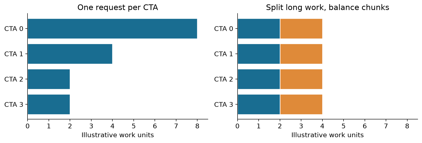
The toy in Figure 5 contains sixteen work units and four workers. Any schedule needs at least four units of elapsed work under the idealized model. A one-request-per-worker assignment takes eight because the longest request dominates. Splitting the long requests into two-unit chunks reaches the lower bound, but this picture deliberately excludes coordination costs.

In a real batch, a lower bound is the maximum of average load and the largest indivisible chunk:

$$T_{\min}\ge \max\left(\frac{\sum_j t_j}{C},\max_j t_j\right). \tag{12}$$

Reducing chunk size improves this bound but increases the number of partial states. The useful optimum sits between insufficient parallelism and excessive decomposition. Short requests can bypass partial-output storage when no reduction is needed, as Appendix D.2 explains.

6.3 Static launch, dynamic metadata

CUDA Graph replay benefits from stable launch structure and pointers. FlashInfer puts evolving sequence-length-dependent work queues and reduction maps inside a preallocated workspace. The graph can replay the same execution structure while the contents of that workspace change.

The paper separates a CPU plan from GPU run. Planning executes per generation step; compatible layers reuse it. The workspace contains pinned-host staging data, GPU metadata, and partial outputs. Section 3.3 describes attention and contraction stages and also mentions merging stages into a persistent kernel; its wording is not enough to infer the precise synchronization protocol of every execution configuration. The stable interface is clearer than that implementation detail.

6.4 Algorithm 3: conceptual serving-step lifecycle

This describes Listing 1’s contract, not a ready-to-run API recipe.

1. Choose upper bounds and allocate persistent workspace.
2. Prepare specialized kernels and graph configurations.
3. Capture GPU run operations with stable buffer addresses.
4. At a generation step, update request lengths and page maps.
5. Select a compatible prepared graph configuration.
6. Plan work and copy metadata into fixed workspace sections.
7. Ensure the copy is ordered before graph execution.
8. Replay the graph; reuse valid plan information across layers.
9. Consume outputs, update request state, and repeat.

“Fixed pointers” does not mean unlimited dynamic capacity. If request count or accumulated lengths exceed the declared bounds, the prepared allocation no longer establishes validity. A serving design needs an explicit capacity transition path; it cannot silently assume graph replay makes all shapes safe.

6.5 The memory cost of splitting

Appendix D.3 gives a partial-output capacity expression

$$E_{\mathrm{partial}}\le 2CT_qH_q(d+1). \tag{13}$$

This counts scalar elements under the paper’s allocation argument; it is not a byte count and excludes scheduler metadata. The extra coordinate holds the log-normalizer. If all stored elements used $s$ bytes, the corresponding estimate would be $sE_{\mathrm{partial}}$; if output and normalizer types differ, they must be counted separately.

For an illustrative $C=100,T_q=16,H_q=32,d=128$, Equation 13 gives 13,209,600 elements, or about 50.4 MiB at four bytes each. This arithmetic is not a reported default allocation. It demonstrates why a “small” intermediate state can become significant when multiplied by tiles, heads, and CTAs.

The claimed factor of two depends on the scheduler’s splitting and write-through argument. It should not be treated as a theorem for any custom partitioning policy. I would separate the paper’s stated capacity contract from a generic design in which arbitrary small chunks could produce many more intermediates.

7. What the experiments establish

7.1 Read the environment before the percentages

The paper evaluates FlashInfer v0.2 with CUDA 12.4 and PyTorch 2.4.0 on A100 40GB SXM and H100 80GB SXM, primarily using f16. The main serving study uses SGLang v0.3.4 and a Triton v3.0 attention backend. Llama 3.1 8B runs on one H100; 70B uses four. These comparisons describe that experimental stack.

The workloads are ShareGPT and a synthetic Variable distribution. The main study adjusts request rates to keep P99 TTFT below 200 ms. Figure 7 labels its central latency statistic “Medium,” apparently intending median. I retain the exact labeled values rather than turning an ambiguous caption into an undocumented aggregation rule. The explicit median columns in Appendix Table 8 have a clearer definition.

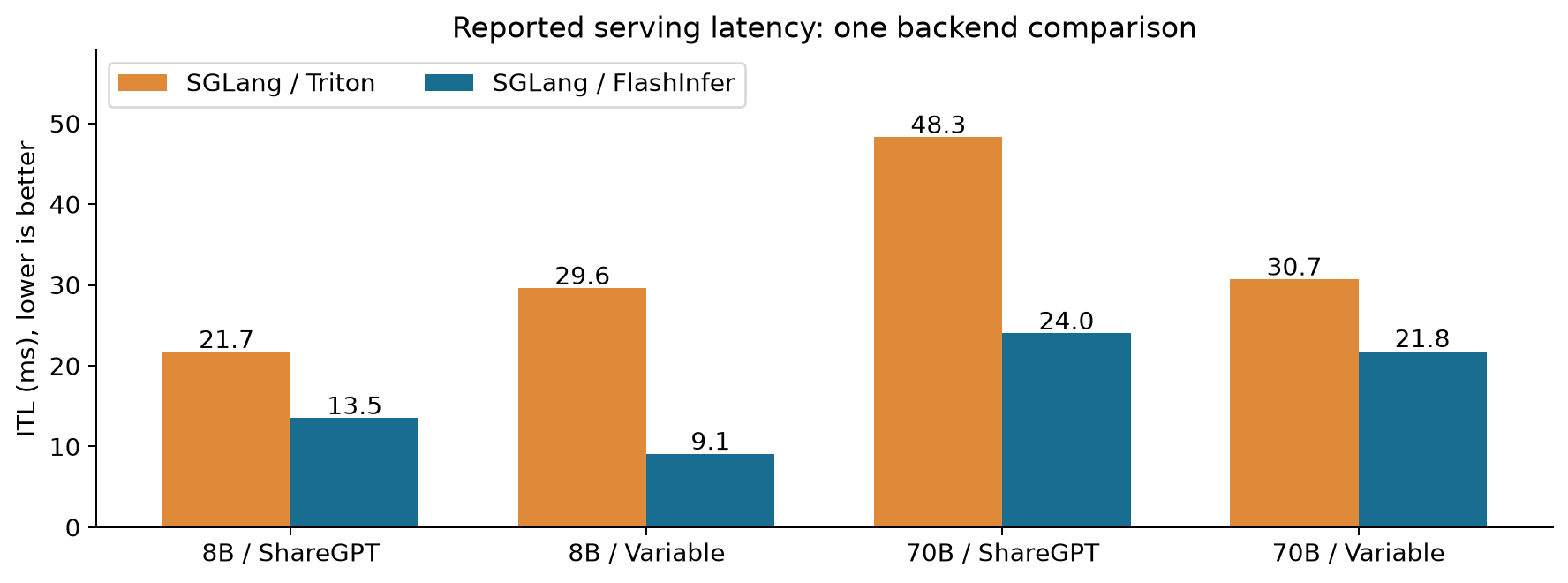
For a baseline latency $t_b$ and new latency $t_n$, distinguish a fractional reduction from a speed ratio:

$$r=1-\frac{t_n}{t_b},\qquad S=\frac{t_b}{t_n}=\frac{1}{1-r}. \tag{14}$$

For 8B on the Variable workload, $29.6$ to $9.1$ ms means a 69.3% reduction, or about $3.25\times$ the inverse-latency ratio. It does not mean a 69.3% throughput increase. For 70B on Variable, $30.7$ to $21.8$ ms is a 29.0% reduction. Those values explain the headline range while showing its dependence on workload.

The corresponding TTFT pairs are 49.2 to 38.8 ms and 61.8 to 53.2 ms for 8B, and 141.2 to 115.6 ms and 165.2 to 157.8 ms for 70B. Improvement in token spacing and improvement in time to first token are distinct outcomes, influenced by different computation and queueing paths.

7.2 Isolate the scheduler with the ablation

Comparing two complete backends changes more than scheduling. Appendix G.3 is more informative about the scheduler itself because it contrasts FlashInfer with and without load balancing. It evaluates Llama 3.1 8B on H100, with fixed 256-token outputs for the two synthetic input distributions.

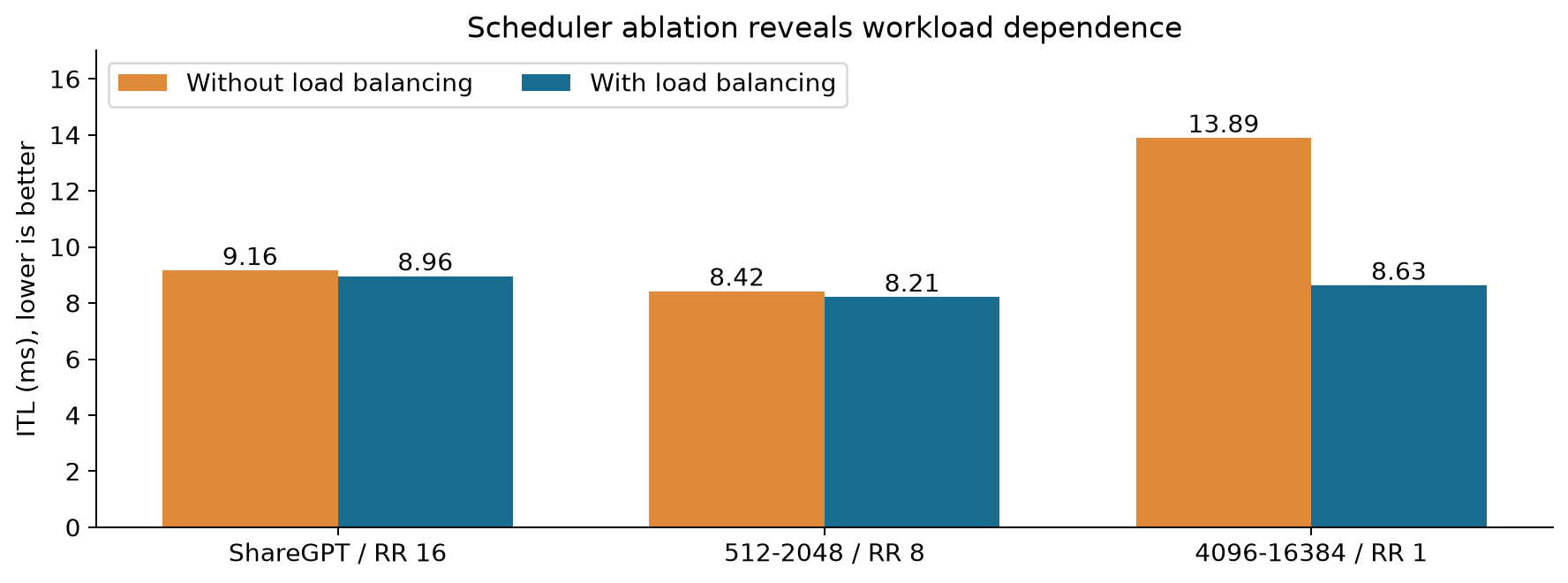
The ITL reductions are about 2.18% for ShareGPT, 2.49% for the short-variable workload, and 37.87% for the long-variable workload. Meanwhile the long-variable TTFT only changes from 421.60 to 411.02 ms, a 2.51% reduction. I interpret this as evidence that removing a decode imbalance can matter greatly without proportionally reducing the prompt-processing path.

Request rates differ across these ablation rows, so the rows are separate workload experiments rather than a controlled curve over sequence length alone. The much smaller short-workload improvements also caution against attributing every main-figure gain to the runtime scheduler.

7.3 Shared-prefix reuse: kernel wins need context

Appendix Table 5 fixes suffix length at 128 and varies shared-prefix length and batch size. At batch 64 and prefix 32,768, kernel latency falls from 4090 to 254.54 microseconds: about $16.07\times$. At batch 16 and prefix 1024, it falls only from 46.52 to 45.17 microseconds: about $1.03\times$.

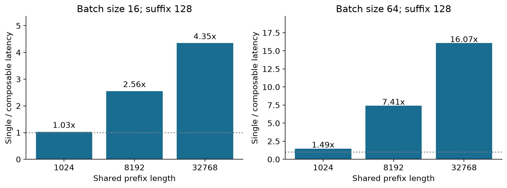
A simple traffic model helps explain the trend. Suppose $n$ queries share $P$ prefix tokens and each has $S$ private tokens. Without cross-query on-chip reuse, a rough KV-read count is $n(P+S)$. With ideal prefix reuse, it is $P+nS$. The possible traffic ratio is

$$R_{\mathrm{traffic}}=\frac{n(P+S)}{P+nS}. \tag{15}$$

It approaches $n$ when the prefix dominates and approaches one when private suffixes dominate. This deliberately ignores cache hits, tile reloads, metadata, and merging. Existing L2 reuse can make the actual baseline traffic lower than this model, so Equation 15 is a mechanism illustration, not a guaranteed speedup ceiling for measured latency.

In end-to-end parallel generation, Figure 10 reports moderate improvements and some regressions. At $n=4$, its ITL labels show 13.73% improvement for 8B and 17.42% for 70B. At $n=1$, the labels are negative: -10.34% and -18.56%. Extra decomposition is not free.

There is a small internal inconsistency worth preserving. The text says the peak is at $n=4$, but the 8B ITL panel labels $n=2$ at +15.95%, larger than +13.73% at $n=4$. I therefore describe $n=4$ as a useful reported point, not an established universal optimum. The interpretation of $n$ is parallel generation branches or completions; it should not be confused with changing autoregressive dependence so that one sequence emits arbitrary future tokens simultaneously.

7.4 Sparse loading has a visible cost

Appendix B compares contiguous KV with page size one. Decode bandwidth is similar in the shown settings, but prefill loses throughput, especially for the FA3 template.

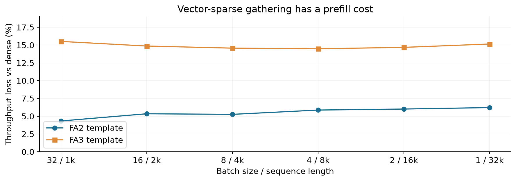
For batch one and length 32,768, the FA2 figures are 370 versus 347 TFLOP/s, a 6.22% throughput reduction. FA3 gives 627 versus 532, a 15.15% reduction. The appendix’s broad “approximately 10%” description hides that template-dependent difference. A throughput reduction also differs from its reciprocal latency increase: 627/532 implies about 17.9% longer kernel time for fixed work.

The explanation is consistent with the design: dense Hopper loading uses TMA, whereas fine-grained arbitrary gathering uses a different copy path and more pointer arithmetic. Sparsity is a useful representation, not automatically a performance improvement when the actual amount of attention work is unchanged.

7.5 Fusion and integration give complementary evidence

Streaming-LLM experiments use Vicuna-13B on MT-Bench. Figure 9 reports fused-RoPE ITL of 13.2, 13.3, and 13.4 ms on H100 for recent-window sizes 1000, 2000, and 4000. The unfused comparison gives 18.2, 19.1, and 20.0 ms. The pointwise reductions are 27.5%, 30.4%, and 33.0%; the prose’s 28–30% range does not cover every displayed point exactly. I prefer the explicit pairs.

Appendix Tables 1–4 compare causal, soft-cap, ALiBi, and sliding-window variants against FlexAttention. They support the value of specialized templates in that environment, but not a timeless ranking of CUDA against Triton. Compiler capabilities and integration change independently of the paper’s conceptual architecture.

The vLLM appendix supplies an important counterexample:

Configuration	Throughput (tokens/s)	Median ITL (ms)	Median TTFT (ms)
Default bf16	6062.89	10.42	35.85
FlashInfer bf16	6065.41	10.63	36.60
Default e4m3	6015.86	12.56	39.74
FlashInfer e4m3	6020.32	10.92	37.93

Table values come from Appendix G.4, Table 8, at request rate 16. bf16 throughput barely changes, while both latency metrics worsen by about 2%. With e4m3 KV, ITL improves about 13.1%. The authors attribute the bf16 regression to host-side Python integration overhead. The table supports the existence of an integration bottleneck; it does not give a complete time breakdown proving that attribution.

8. Limitations and failure boundaries

The paper evaluates a particular generation of software and GPUs. FlashInfer v0.2, SGLang v0.3.4, and the listed compiler versions matter. A reproducible historical comparison does not establish the best backend for a newer model or GPU. Forward inference is the demonstrated scope; customizable backward kernels are future work in the paper.

A unified format still pays for its generality. Pointer gathers, extra index arrays, partial states, and format composition all consume resources. A fully contiguous, uniform prefill batch might prefer the simplest dense path. Very small query counts can fail to provide enough reuse to offset preparation and composition.

The cost model is incomplete. $\alpha l_q+\beta l_k$ cannot directly describe every mask density, cache interaction, GQA layout, quantization conversion, or variant-specific instruction count. A plan can be balanced under its estimate and imbalanced in elapsed GPU time. That is a limitation of the heuristic, not a failure of attention-state algebra.

Capacity and lifetime are part of correctness. Persistent buffers must remain alive throughout graph replay. Metadata updates must be ordered before consumption. The upper bounds used for capture must cover the actual request set. The paper explains the design requirements but does not establish arbitrary-capacity execution with no transition overhead.

Reported summary statistics do not describe all tails. P99 TTFT is used as an operating constraint in the main experiment, but the plotted ITL and TTFT central values do not reveal per-request P99 ITL, fairness between short and long requests, or behavior during bursts. The absence of confidence intervals in the shown tables also limits interpretation of two-percent differences.

A fast sparse kernel does not validate a pruning policy. Appendix G.5 evaluates Quest-style fine-grained sparsity. The latency numbers show efficient evaluation of selected pages. Whether discarded pages preserve generation quality is a separate question requiring model-level evaluation of the selection method.

9. Independent critical analysis: optimize the execution boundary

9.1 The central contribution is a separation of timescales

My strongest takeaway is that different facts should be fixed at different times. Operator algebra and hardware tile capabilities change infrequently and belong in specialization. Request lengths and page membership change per step and belong in metadata. Tensor values change at every layer and belong in the GPU execution path.

This separation explains why “just compile the attention” is incomplete. Compiling every request shape can produce too many variants; treating every property as dynamic can waste optimization opportunities. FlashInfer offers a practical middle point. Its sparse views and attention states act as interfaces between components with different lifetimes.

A useful consequence is that cache ownership can remain with the serving framework. The attention engine consumes a view of that ownership instead of becoming a second memory manager. That reduces integration coupling, but it increases the importance of a precise contract for positions, shared pages, graph capacity, and plan reuse.

9.2 Derive a break-even condition for planning

Consider $L$ compatible attention layers per generation step. Suppose the unscheduled attention time per layer is $u$, the scheduled computation plus merge time is $v$, the CPU planning and metadata-transfer critical-path cost is $p$, and any newly exposed integration overhead is $h$.

The two step-time contributions are

$$T_{\mathrm{base}}=Lu,\qquad T_{\mathrm{planned}}=Lv+p+h. \tag{16}$$

The transformation helps when

$$L(u-v)>p+h. \tag{17}$$

This is my simplified model, not the paper’s measured timing model. It clarifies why amortization across layers is valuable and why a small kernel win may disappear inside a host-heavy serving stack. If plan reuse is invalid because layers have different visible lengths or layouts, $p$ may be paid more often and the inequality changes.

For illustration, let $L=32$, a per-layer saving of two microseconds, and $p+h=30$ microseconds. The net saving is 34 microseconds per step. If the per-layer saving falls to half a microsecond, the same integration becomes 14 microseconds slower. No GPU experiment is being claimed; the example exposes the scale that a measurement must resolve.

9.3 Amdahl’s law prevents a kernel result from becoming a serving promise

Let $f$ be the fraction of baseline step latency spent in the optimized attention path, and let that path speed up by $s$. Ignoring new overhead,

$$S_{\mathrm{step}}=\frac{1}{(1-f)+f/s}. \tag{18}$$

At $f=0.2,s=16$, the whole-step speedup is only about $1.23\times$. Thus the $16.07\times$ shared-prefix kernel ratio can coexist with much smaller end-to-end gains. A serving evaluation should report both $f$ and the newly added costs rather than ask readers to infer them from a headline.

9.4 What would make the empirical argument stronger?

I would use a paired experiment that holds arrival traces, model weights, cache policy, precision, and graph configuration fixed. First compare dense versus indexed loading at equal visible token counts. Then vary scheduling while keeping the microkernel fixed. Finally vary prefix composition while retaining the same physical cache allocation. This isolates representation cost, balancing benefit, and reuse benefit.

The response variables should include device attention time, CPU planning time, metadata transfer, merge time, workspace high-water mark, TTFT, ITL, and completed-request throughput. Tail latency and short-request fairness should accompany medians. Repeated trials are especially important where the reported change is only a few percent.

9.5 Algorithm 4: a proposed research protocol

This is a proposed evaluation design, not work performed in this review and not a procedure for checking the authors’ source.

1. Fix one request-arrival trace, model, precision, and cache policy.
2. Define dense/uniform, ragged, skewed, and shared-prefix cases.
3. Pair conditions that differ in exactly one optimization.
4. Warm up each prepared configuration under the same policy.
5. Repeat the same trace and record host, device, and user metrics.
6. Include planning, data transfer, merge, and workspace costs.
7. Report distributions and uncertainty, including regressions.
8. Separate kernel ratios from end-to-end latency reductions.

I would additionally sweep prefix length and branch count jointly. A single branch count cannot summarize reuse. The ratio $P/S$, the fraction of the step spent in attention, and the real cache-hit behavior can change the threshold at which composition becomes worthwhile.

For graph-compatible execution, the interesting experiment is a controlled transition across capacity boundaries. A steady-state replay benchmark omits graph preparation, buffer growth, and configuration switches. Those costs need not dominate, but measuring them would make the dynamic-workload claim more operationally complete.

9.6 My judgement

The paper convincingly demonstrates that attention engines should consume structured workload information rather than accept only dense tensor shapes. The algebraic foundation is clear, the reuse opportunities are concrete, and the appendix supplies useful negative results. Its strongest generalizable result is the architecture: reusable state composition plus independent layout, template, and schedule decisions.

The main uncertainty is attribution and portability of the measured gains. Backend comparisons combine multiple design choices, and the software stack is historical. The vLLM result shows that integration overhead can reverse a kernel advantage. I would adopt the design principles with confidence while treating a particular speedup as a workload-specific hypothesis.

10. Conclusion

FlashInfer makes attention fit serving by exposing three things that a dense shape hides: physical KV access, shared computation opportunities, and unequal request work. Attention states let the engine decompose the problem without discarding normalization information. Sparse views keep memory ownership separate from execution. Runtime plans balance changing work while prepared kernels and buffers remain stable.

The decision rule I take away is practical: identify the bottleneck, estimate the reuse or imbalance that can be removed, and include the new planning and merge costs. Long skewed requests and large shared prefixes offer strong opportunities. Uniform short workloads and host-heavy integrations require more caution. That conclusion is supported by both the positive results and the counterexamples in the paper.

References and figure provenance

• Ye et al. FlashInfer, arXiv:2501.01005v2, MLSys 2025. Full 21-page document including Appendices A–G is the primary source. Sections 2–3 support the mathematical and architectural explanations; Section 4 and Appendix G supply experiments.
• FlashInfer project and official repository are resource pointers.
• Figures 1–5 are original explanatory diagrams or analytic examples derived from the paper’s concepts. Their numbers are illustrative.
• Figure 6 redraws paper Figure 7; Figure 7 redraws Appendix Table 6; Figure 8 calculates ratios from Appendix Table 5; Figure 9 calculates throughput losses from paper Figure 12. Captions distinguish redraws from original examples.
• All new equations, toy schedules, break-even calculations, and research proposals in this review are explanatory analysis. They are not model runs, benchmark reproductions, or claims about unseen experimental results.