Attention Residuals: Learning What to Retrieve Across Network Depth

Review date: 2026-09-19
Author: Zhongzhu Zhou
Paper reviewed: Attention Residuals
Paper authors: Kimi Team; Guangyu Chen, Yu Zhang, Jianlin Su and collaborators; the complete contribution list is in Appendix A.
arXiv: 2603.15031v1, submitted 2026-03-16
this review uses the 21-page v1, including Appendices A and B.

1. What changes when a residual becomes a retrieval operation?

I read Attention Residuals as a proposal about the interface between layers. A conventional residual stream carries an accumulated vector forward. Each attention or feed-forward sublayer adds a new contribution, and subsequent sublayers receive the sum. AttnRes instead preserves earlier outputs as individually addressable sources and learns how much of each source the next sublayer should receive. The selection varies with the token, even though the query is a learned parameter that stays fixed after training.

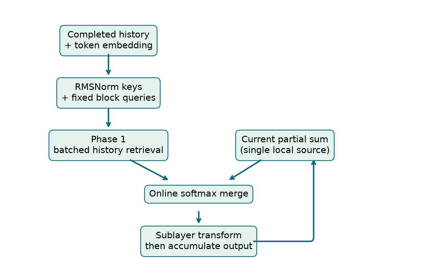
That last detail connects the mathematical design to the systems design. A query produced from the current hidden state would be more expressive, but it could not be evaluated before that state existed. A fixed query can score all already completed sources in advance. The paper uses this independence to batch retrieval for several future layers, then merges those results with the evolving local state. The architecture and the execution schedule are therefore closely related.

The strongest result is not simply that another attention operator improves a benchmark. The paper provides a route from full access to every earlier output, through compressed block histories, to a distributed execution plan. The main 48B-total, 3B-activated model uses nine residual blocks across 54 sublayers and an additional embedding source. Its comparison with the baseline follows the same 1.4T-token recipe. Table 3 shows improvements on fourteen of fifteen benchmarks, with MMLU-Pro tied at the displayed precision.

Three distinctions guide this review. First, source selection is token dependent, but it happens over depth rather than over sequence positions. Second, the block architecture approximates the full architecture; the two-phase schedule is an exact rearrangement of the chosen architecture in real arithmetic. Third, lower validation loss at a fixed training-compute budget is not a measured reduction in elapsed training time. Keeping these distinctions explicit makes the paper more useful for architecture decisions.

2. Prerequisites: residual streams, normalization, and two different axes

Let $d$ be the hidden width, $T$ the number of tokens, and $B$ the batch size. A hidden-state tensor has shape $B\times T\times d$. I write most equations for one token, so each source is a vector in $\mathbb R^d$. The same mixing rule is independently applied to each token, while the underlying attention sublayer can still mix information across sequence positions.

The paper counts an attention sublayer and an MLP sublayer as two separate layers. I use $L$ for this sublayer count and $L_b=L/2$ for the number of ordinary Transformer blocks. This matters when comparing the 16-block ablation model, which has 32 sublayers, with a residual block size $S=4$. That setting has eight AttnRes blocks, not four.

For standard residuals, let $h_l$ enter sublayer $l$, with its transformation denoted by $f_l$. Expanding the recurrence gives

$$h_{l+1}=h_l+f_l(h_l),\qquad h_l=h_1+\sum_{i=1}^{l-1}f_i(h_i).$$

The expansion reveals a second function of a residual connection beyond its role in optimization: it defines a depth-aggregation rule. Every previous output has coefficient one. A later sublayer can transform the accumulated state, but it cannot directly request one earlier output from the sum unless that information remains recoverable in the representation.

The familiar gradient argument is also worth retaining. Writing $J_i=\partial f_i/\partial h_i$, the Jacobian from one depth to another includes

$$\frac{\partial h_L}{\partial h_l} =(I+J_{L-1})\cdots(I+J_l).$$

Its algebraic expansion contains an identity term. That is a path, not a guarantee that every singular value of the full Jacobian stays near one: other terms can amplify or cancel. Similarly, replacing the residual sum with attention changes the gradient structure; it does not automatically preserve a unit-weight identity path to every source.

PreNorm places normalization before a sublayer transformation, while the accumulated stream itself can grow. A useful simplified normalization is

$$\operatorname{RMSNorm}(v) =g\odot\frac{v}{\sqrt{\|v\|_2^2/d+\epsilon}},$$

where $g$ is a learned scale and $\epsilon>0$ prevents division by zero. This operator controls the scale presented to a transformation. It does not by itself constrain the norm of an unnormalized sum elsewhere in the network.

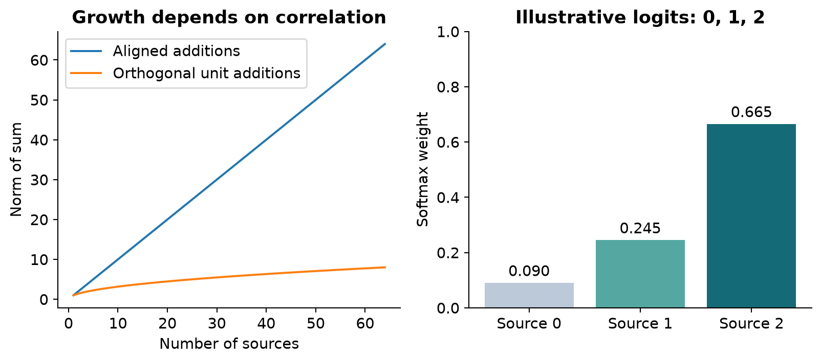
I treat the paper’s depth-growth discussion as a motivation rather than a universal growth law. If $k$ unit vectors align, their sum has norm $k$; if they are orthogonal, it has norm $\sqrt{k}$. Cancellation can reduce it further. Actual growth depends on learned correlations and magnitudes. The empirical curves in paper Figure 5 are stronger evidence for this model family than asserting linear growth for every possible residual network.

3. Full AttnRes: derive the mixture before interpreting it

Define $v_0=h_1$ and $v_i=f_i(h_i)$ for $i\geq1$. The input to sublayer $l$ is reconstructed from $v_0,\ldots,v_{l-1}$. Each destination has a learned pseudo-query $w_l\in\mathbb R^d$. The score and weight are

$$z_{li}=w_l^\top\operatorname{RMSNorm}(v_i),\qquad \alpha_{li}=\frac{\exp(z_{li})}{\sum_{j=0}^{l-1}\exp(z_{lj})},$$

followed by

$$h_l=\sum_{i=0}^{l-1}\alpha_{li}v_i.$$

There is no extra $1/\sqrt d$ factor in the paper’s displayed scoring definition. The learned query can absorb a scale, but that does not justify silently changing the stated rule when explaining it. Keys are normalized; values are the original outputs. Consequently, a large output does not get a larger logit solely because of its norm, yet its magnitude still affects the resulting weighted sum.

Why is the mixture input dependent if the query is fixed? Because each key depends on the input token and all preceding computation. Two tokens can produce different $v_i$, hence different logits and different mixture weights under the same $w_l$. What is deliberately removed is the dependence of the query on the current layer’s not-yet-computed state.

Softmax creates competition: increasing one logit reduces the normalized weights of other sources. For the illustrative logits $(0,1,2)$, the weights are approximately $(0.090,0.245,0.665)$. Adding the same constant to all three logits changes nothing because the common exponential factor cancels. Multiplying all logits by a positive constant does change their sharpness. Query norm and key normalization therefore participate in the selectivity of the mechanism.

The initialization is important. The paper initializes every pseudo-query to zero. Initially all logits are zero and

$$\alpha_{li}=1/l,\qquad h_l=\frac1l\sum_{i=0}^{l-1}v_i.$$

This is a uniform average, not the original unit-weight residual sum. PreNorm can reduce the practical effect of a common scale under idealized assumptions, but normalization includes $\epsilon$, learned scales, and downstream nonlinearities. I would not describe zero initialization as exact functional preservation of a pretrained standard-residual checkpoint. The reported experiment trains the modified architecture.

Because the weights are nonnegative and sum to one, the mixed input satisfies the convexity bound

$$\|h_l\|_2\leq\sum_i\alpha_{li}\|v_i\|_2 \leq\max_i\|v_i\|_2.$$

The first inequality is the triangle inequality; the second uses normalized nonnegative weights. This controls the aggregation relative to its sources. It does not bound the sources themselves or every network Jacobian. That narrower claim is sufficient to explain why replacing repeated unweighted accumulation can change the observed magnitude profile.

Algorithm 1: Full depth retrieval for a single token.

1. Initialize the source list with the token embedding $v_0$.
2. At sublayer $l$, normalize every available source to form keys; keep original sources as values.
3. Score those keys with $w_l$. Subtract the maximum score before exponentiating.
4. Divide exponentials by their sum and form the weighted value sum $h_l$.
5. Evaluate the sublayer transformation $f_l(h_l)$ and append its output as the next source.
6. Repeat in depth order; use the corresponding final aggregation for the model output.

This algorithm exposes the expense: there are $1+2+\cdots+L$ source visits. Ignoring batch and token factors, arithmetic is $O(L^2d)$ and stored source vectors require $O(Ld)$. Small parameter overhead should not be confused with small activation traffic.

4. Block AttnRes: choose what information to discard

Partition the sublayers into $N$ consecutive blocks of size $S=L/N$, assuming divisibility for now. For block $n$, define its completed summary and its partial summary after $i$ sublayers as

$$b_n=\sum_{j\in\mathcal B_n}f_j(h_j),\qquad b_n^{(i)}=\sum_{j\in\mathcal B_n\text{, first }i}f_j(h_j).$$

The embedding remains a separate source $b_0=h_1$. The first sublayer in block $n$ attends to $b_0,\ldots,b_{n-1}$. Subsequent sublayers also attend to the one evolving partial sum $b_n^{(i-1)}$. The partial sum is absent before the first transformation; adding a zero-valued placeholder to softmax would add probability mass and change the result.

The important algebra is what happens when a block summary receives weight $\alpha_n$:

$$\alpha_n b_n=\sum_{j\in\mathcal B_n}\alpha_n f_j(h_j).$$

Every output in the completed block receives the same effective coefficient. Full AttnRes can emphasize one output and suppress another. Block AttnRes cannot do that after they have been summed. Opposing contributions can cancel, and no later choice of block weight can recover the canceled components. The block approximation is therefore a lossy representation decision, not merely a faster way to calculate the full model.

Algorithm 2: Block retrieval and summary construction.

1. Set the completed-history list to $[b_0]$.
2. At the beginning of each block, initialize the partial sum $p=0$ and the local sublayer counter $i=1$.
3. Use completed history as the source set; include $p$ only when $i>1$.
4. Normalize source keys, score them using the destination’s pseudo-query, and softmax over this entire source set.
5. Form the weighted input $h_l$ and evaluate $y_l=f_l(h_l)$.
6. Update $p\leftarrow p+y_l$, then advance the local counter.
7. At the boundary, append $p$ to history and start a new empty partial sum. If the final block is shorter, store its actual final sum.
8. After all sublayers, aggregate completed sources for the final output using the model’s output query.

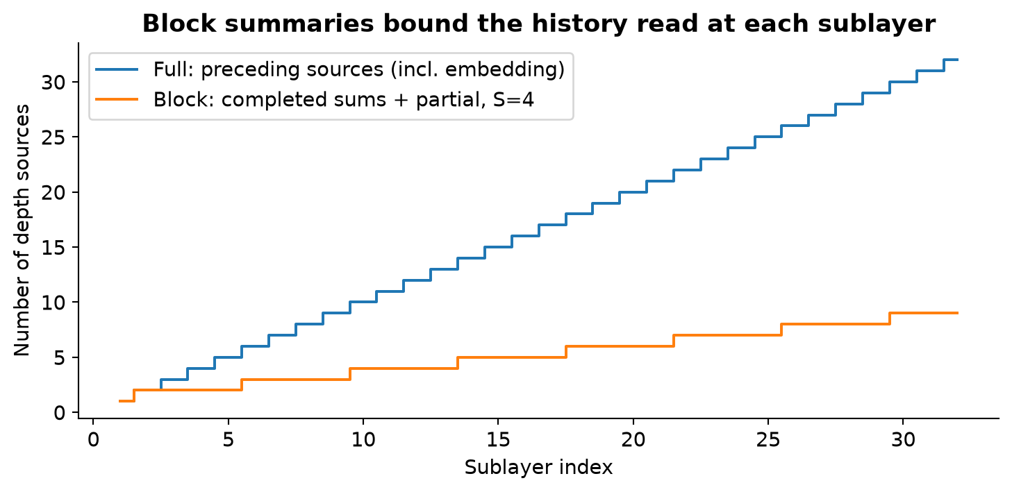
The architectural history becomes $O(Nd)$ per token, plus local workspace. Each of $L$ sublayers consults at most roughly $N$ sources, so a useful general arithmetic bound is $O(LNd)$. The paper sometimes describes this as $O(N^2)$ while its related-work discussion gives $O(LN)$. These agree up to a fixed factor only when $S=L/N$ is held constant. When block size is a variable, retaining both $L$ and $N$ avoids hiding its cost.

There are two revealing endpoints. If $S=1$, every completed block contains exactly one output and the full architecture is recovered. If $N=1$, all previous outputs share one accumulating block, while the embedding remains separate. This is residual-like accumulation inside a block, but the displayed attention formula still mixes the embedding with the partial sum using normalized weights. It is not generally identical to the standard unweighted sum. I interpret the paper’s statement about recovering residuals at $N=1$ as a structural analogy unless extra scaling conditions are supplied.

For a concrete information-loss example, consider two outputs $(1,0)$ and $(-1,1)$. Their block sum is $(0,1)$. Full retrieval can assign weights $0.8$ and $0.2$, producing $(0.6,0.2)$ before considering other sources. A single scalar times the block sum cannot produce a nonzero first component. Normalizing keys does not restore the missing direction. This example isolates the approximation without making any claim about how often cancellation occurs in trained models.

5. Exact two-phase attention: keep the denominator

At the start of a block, completed history is known and all $S$ pseudo-queries are already known. Phase 1 scores that history for all $S$ future destinations in parallel. The partial sum is not yet known, so phase 2 processes it sequentially. To combine the two results correctly, one must preserve softmax normalization statistics.

For any source subset $A$, define a stable representation

$$m_A=\max_{i\in A}z_i,\qquad \ell_A=\sum_{i\in A}e^{z_i-m_A},\qquad o_A=\sum_{i\in A}e^{z_i-m_A}v_i.$$

Here $o_A$ is an unnormalized weighted numerator and $\ell_A$ is a scaled denominator. The normalized answer is $o_A/\ell_A$. I use this notation consistently because a log-sum-exp value is a different quantity: $\operatorname{LSE}_A=m_A+\log\ell_A$. The paper’s Algorithm 1 uses a division by $\ell$ and exponential rescaling; that algebra requires the scaled-sum interpretation even though its annotation mentions LSE.

For disjoint subsets $A$ and $D$, choose $m=\max(m_A,m_D)$. Multiplying each numerator and denominator by its missing scale gives

$$o=e^{m_A-m}o_A+e^{m_D-m}o_D,$$ $$\ell=e^{m_A-m}\ell_A+e^{m_D-m}\ell_D, \qquad h=o/\ell.$$

To derive this, expand the first term: $e^{m_A-m}o_A=\sum_{i\in A}e^{z_i-m}v_i$. The second term gives the corresponding sum over $D$. Their union therefore has exactly the numerator and denominator of a single softmax over all sources. No approximation enters this identity. Floating-point reduction order can still cause small numerical differences.

An example shows why averaging normalized partial results fails. Suppose $A$ has logits $0$ and $\log2$ with scalar values $2$ and $5$. Its unscaled denominator is $3$, its numerator is $12$, and its normalized output is $4$. A new source has logit $\log3$ and value $8$, giving denominator $3$ and numerator $24$. The union output is $(12+24)/(3+3)=6$. Equal averaging happens to work here only because both groups have the same total exponential mass. If the new logit were $\log6$, the union would instead be $(12+48)/(3+6)=20/3$, while an equal average would incorrectly remain $6$.

Algorithm 3: Two-phase execution of one Block AttnRes block.

1. Stack its destination pseudo-queries into $Q\in\mathbb R^{S\times d}$.
2. Normalize completed source keys and calculate all historical attention statistics $(o_l^{H},m_l^{H},\ell_l^{H})$ in one batched operation.
3. Initialize the partial sum $p=0$.
4. For the first local sublayer, use $h_l=o_l^{H}/\ell_l^{H}$; do not create a fictitious local source.
5. For each later sublayer, compute the score of $p$. Its singleton statistics are $(o_l^{P},m_l^{P},\ell_l^{P})=(p,z_l^P,1)$.
6. Merge historical and singleton statistics with the stable formulas above, then divide numerator by denominator.
7. Evaluate $f_l(h_l)$ and add the output into $p$ before the next sublayer.
8. Store the completed $p$ when the block ends.

The completed-history work can be batched, but the partial-sum loop remains sequential. A paper discussion of parallel queries should therefore not be read as parallel execution of all nonlinear layers. The speed benefit comes from reusing memory reads and improving the shape of computation, while respecting the same causal dependency in depth.

6. Distributed training: count transfers, then ask about overlap

Full AttnRes can reuse activations already retained in simple backpropagation. Activation checkpointing changes that comparison: a conventional model may discard those activations and recompute them later, whereas later depth retrieval still needs the sources. Pipeline parallelism adds another constraint because a source created on an earlier stage may be needed on later stages. The paper’s systems work addresses this large-scale regime.

Let $P$ be the number of physical pipeline ranks, $V$ the number of virtual stages per rank, and $C=PV$ the total logical chunks. Use the paper’s simplified average $N_p$ for new block representations per chunk in the transfer model. If transition $j$ sends all $jN_p$ accumulated blocks, summing transition costs gives

$$\operatorname{Comm}_{\rm naive} =N_p d\sum_{j=1}^{C-1}j =\frac{C(C-1)}2N_p d.$$

The factor $BT$ and element size must be restored when calculating actual bytes. Blocks need not align perfectly with pipeline boundaries; $N_p$ is an averaged accounting device rather than a claim that every stage creates an identical integer number of blocks.

With physical-rank caching, a rank retains history from its earlier virtual-stage visit. The first traversal still accumulates history normally. Later traversals only transfer representations created since the receiver’s previous visit. The paper obtains

$$\operatorname{Comm}_{\rm cache} =\left[\frac{P(P-1)}2+(V-1)P^2\right]N_p d.$$

For $P=4,V=2$, the two simplified totals are $28N_pd$ and $22N_pd$. The saved six units agree with the paper’s illustrative reduction. They imply a reduction of about 21.4% in this transfer model, not an eightfold end-to-end speedup. At $V=1$, the formulas coincide because there has been no earlier virtual visit whose cached data can be reused.

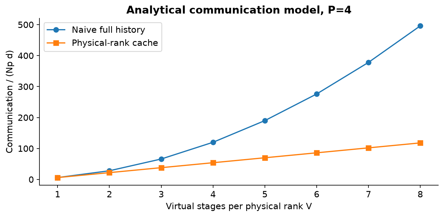
The paper also argues that peak transition traffic changes from dependence on $C$ to dependence on $P$. This can make communication overlap with computation feasible. Whether it actually disappears from the critical path depends on network bandwidth, message latency, microbatch size, scheduling, and the duration of each compute segment. The report gives less than 4% measured training overhead under pipeline parallelism. I treat that as a result for its setup, not as a hardware-independent upper bound.

Cache identity must conceptually include the microbatch and sequence segment; a source from another microbatch is not reusable merely because it has the same block index. Similarly, backward propagation must account for contributions through reused history. These are consequences of the algorithm’s dependency graph, not claims about a particular software implementation. The useful design principle is to remove repeated transfers of the same mathematical object without confusing object reuse with recomputation or cross-example reuse.

7. Inference: distinguish source storage, traffic, and latency

The paper’s Table 1 compares memory access associated with the residual mechanism only. It excludes the internal traffic of attention and MLP transformations. Its representative setting is $L=128,N=8,S=16$, with four streams for mHC. Standard residual merging costs $3d$ elements, Block AttnRes $5.5d$, scheduled Full AttnRes $24d$, and mHC approximately $34d$, omitting small scalar terms in the last figure.

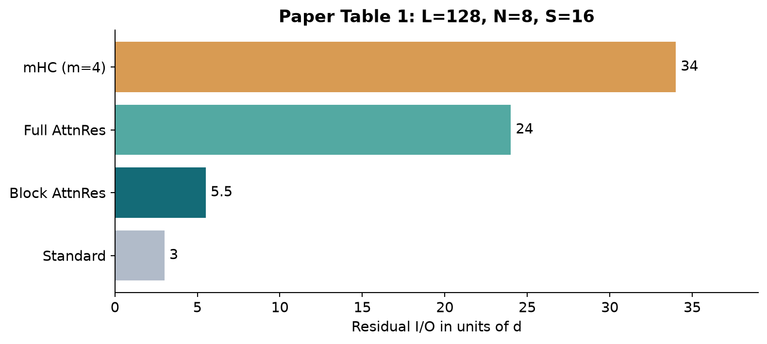
Appendix B explains the Full AttnRes result. This use of blocks is purely an execution schedule: individual layer outputs remain available. In scheduling block $n$, there are $(n-1)S$ historical sources, and keys plus values cost $2(n-1)Sd$ reads. Summing over blocks gives

$$R_H=\sum_{n=1}^{N}2(n-1)Sd=dL(N-1).$$

Within each block, the local sequential reads sum to

$$R_P^{\rm block}=\sum_{t=1}^{S}2(t-1)d=S(S-1)d.$$

Across $N$ blocks, divide $R_H+NR_P^{\rm block}$ by $L=NS$. The amortized reads become $(N+S-2)d$. Add two output writes per sublayer to obtain $(N+S)d$. With $N=8,S=16$, that is $24d$.

The resulting expression has an instructive optimum. If the schedule can choose real-valued $S$ temporarily, its factor is $S+L/S$. Differentiating gives $1-L/S^2=0$, so the continuous minimum is near $S=\sqrt L$. Actual choices must respect integer block sizes, hardware tiles, memory capacity, and sequential latency. This is a scheduling observation, not a prescription for the Block AttnRes architecture, where changing block size also changes the learned function.

Block AttnRes replaces historical individual sources with summaries. The paper’s accounting becomes $(N/S+5)d$. At the illustrative setting, $8/16+5=5.5$. Compared with standard residual traffic, this is about $1.83$ times as much residual I/O, yet the paper reports under 2% end-to-end inference overhead on typical workloads. There is no contradiction: residual traffic is only a fraction of total work, and batching, fusion, and overlap can reduce its wall-clock visibility. Conversely, the comparison $34/5.5$ must not be presented as a measured sixfold speedup over mHC.

Prefill creates a different memory issue. Keeping $N$ summaries for $T$ tokens requires $NTd$ elements, or $bNTd$ bytes for an element size of $b$. Sequence-sharding those summaries across $P$ devices reduces the per-device term to $bNTd/P$. The paper’s rounded 128K-context example goes from 15 GB to about 1.9 GB with eight-way sharding. Restricting active work to a 16K chunk gives another factor of eight, approximately 0.234 GB for this isolated term.

That calculation does not include weights, sequence-attention KV caches, recurrent states, communication buffers, or peak temporary workspace. It is also not a claim that total prefill memory falls by 64 times. The depth history is conceptually different from the sequence KV cache: the former retrieves representations at one token across layers, while the latter allows an attention layer to consult preceding tokens. A hybrid KDA/MLA model can contain both kinds of state.

8. What the scaling and downstream results establish

Table 2 contains five activated non-embedding model sizes: 194M, 241M, 296M, 436M, and 528M. Their token budgets range from 38.7B to 119.0B. At each size, the compared methods share a training configuration, use an 8192-token context, and follow a cosine learning-rate schedule. The configurations across sizes differ, so the plotted line is a family of matched comparisons rather than a fixed-token parameter sweep.

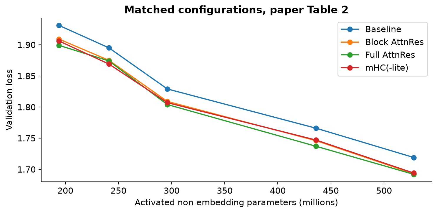
At 528M, baseline loss is 1.719, Block AttnRes 1.693, and Full AttnRes 1.692. The block variant therefore recovers $0.026/0.027\approx96.3\%$ of the loss reduction at this particular point. At 436M, it recovers $0.020/0.029\approx69.0\%$. “Most of the gain” is a reasonable local description, but the fraction varies with scale; it is not a single universal compression-efficiency constant.

The fitted curves are reported as

$$\mathcal L_B(C)=1.891C^{-0.057},\quad \mathcal L_{\rm block}(C)=1.870C^{-0.058},\quad \mathcal L_{\rm full}(C)=1.865C^{-0.057}.$$

Here $C$ is compute in PFLOP/s-days. To compare compute at a target loss $\ell_*$, invert a fitted curve:

$$\ell_*=AC^{-a} \Longrightarrow C^a=A/\ell_* \Longrightarrow C=(A/\ell_*)^{1/a}.$$

This is how to interpret the reported approximately 1.25-times advantage. The small exponent makes the inferred ratio sensitive to rounded fit coefficients and target loss. It is an interpolation-based efficiency statement, without a disclosed confidence interval, rather than proof of the same advantage at arbitrary scale or on a different accelerator.

The large-model experiment is separate. It uses Kimi Linear with 27 Transformer blocks, 48B total and 3B activated parameters, eight routed experts selected from 256 plus one shared expert, and a 3:1 interleaving of KDA and MLA. Six sublayers per AttnRes block produce nine summaries plus the embedding. The main recipe uses 4096-token context, Muon, an 8M-token global batch, a 1T-token warmup-stable-decay pretraining phase, and roughly 400B high-quality mid-training tokens. The report also describes extension to 32K context.

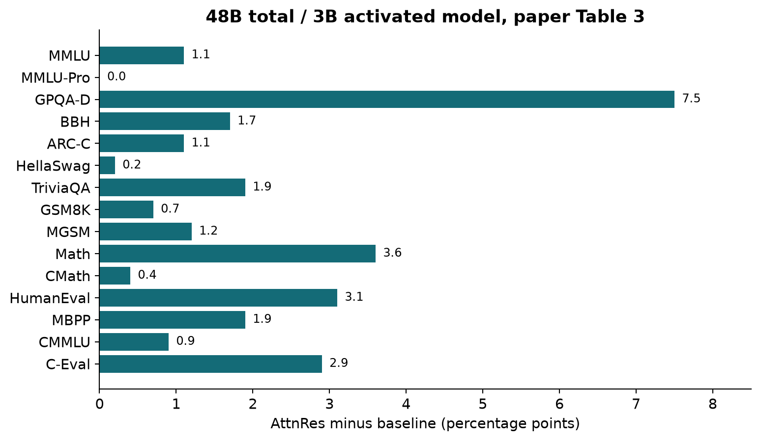
The clearest gains include GPQA-Diamond at +7.5 percentage points, Math at +3.6, HumanEval at +3.1, and C-Eval at +2.9. MMLU improves by 1.1 and HellaSwag by 0.2. The pattern is compatible with a benefit to compositional processing, but it does not isolate a causal mechanism: the architecture changes optimization, representation scale, and access to earlier features together. Benchmark improvements alone cannot assign the gains to just one of these effects.

The training curves show lower validation loss, reduced depth-dependent output growth, and more even gradient magnitudes. Those observations reinforce the motivation. They are not substitutes for multiple random seeds, controlled causal interventions, or uncertainty estimates. In particular, a large improvement on a smaller benchmark should prompt attention to sampling and evaluation protocol before being treated as an exact estimate of general reasoning improvement.

9. Design choices: what was bought, and what was given up?

The ablations are unusually useful because the most expressive option is not the default. Full AttnRes with an input-dependent query reaches loss 1.731, compared with 1.737 for the fixed-query version. The paper chooses fixed queries to avoid a $d\times d$ projection per sublayer and to retain advance batching over completed history. The choice therefore sacrifices some demonstrated modeling quality for a better execution structure.

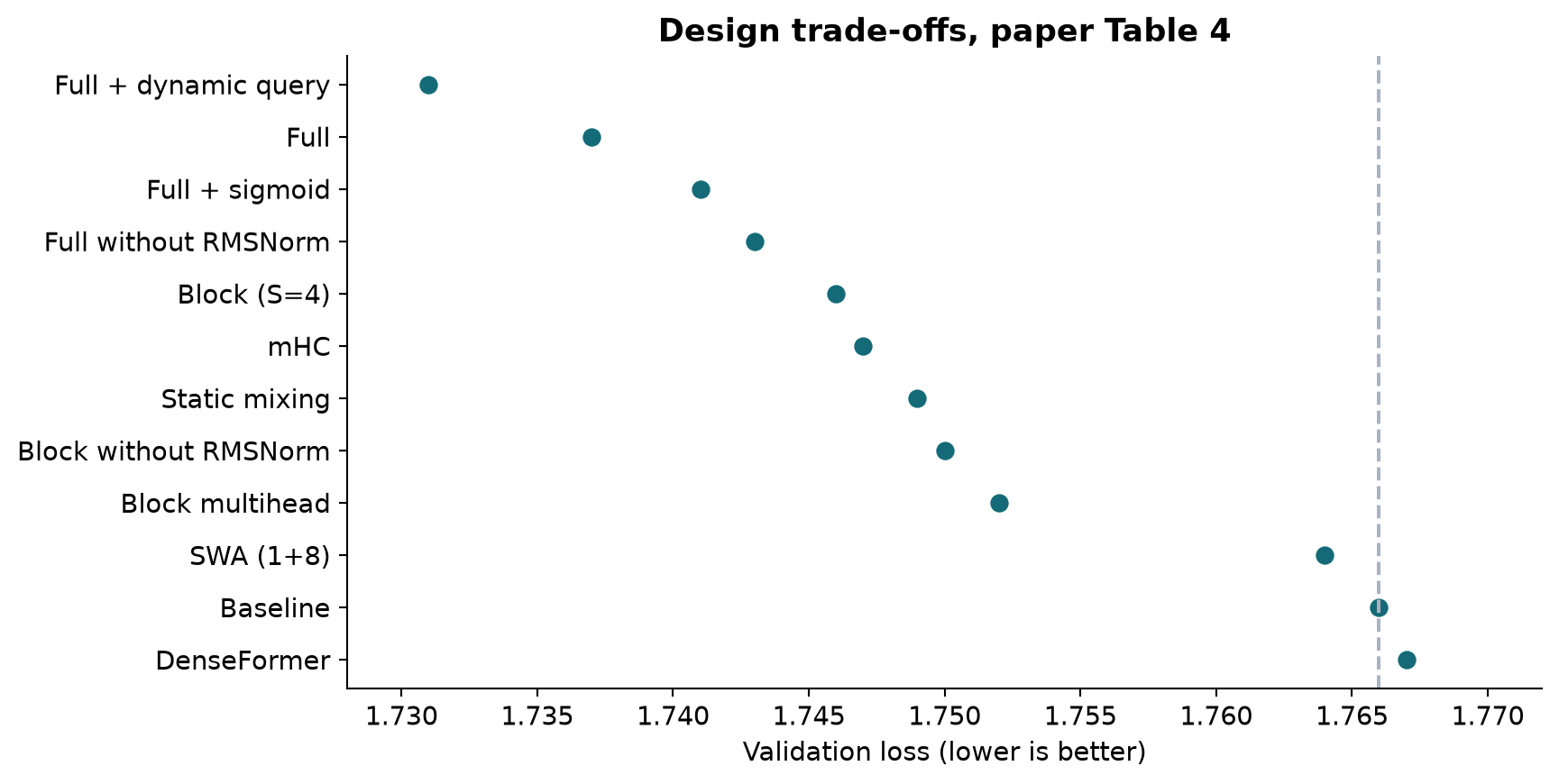
Static mixing gives 1.749, compared with 1.737 for Full AttnRes. This supports content-dependent source selection under the tested recipe. It does not establish that every static-mixture design must fail; DenseFormer and static coefficients have their own optimization choices, and only the listed configurations were tested.

Replacing softmax with sigmoid gives 1.741. Competitive normalization is a plausible explanation for the difference: independently activated sigmoid gates need not sum to one, so both scale and selection change. A stronger causal comparison would normalize sigmoid gates or explicitly match mixture norms, separating competition from overall magnitude control.

Removing key RMSNorm changes Full loss to 1.743 and Block loss to 1.750. This is consistent with the need to prevent source norm from determining retrieval scores, especially when complete blocks and partial blocks contain different numbers of outputs. However, the values remain unnormalized, so key normalization cannot remove all magnitude effects from the downstream signal.

Multihead block mixing reaches 1.752 versus 1.746 for the single-head block variant. The paper interprets this as support for whole-vector relevance. I regard that as one hypothesis. Different head widths, optimization sensitivity, or reduced cross-channel coordination could also explain the degradation. One multihead setting is not enough to establish that token features universally share the same preferred depth source.

The sliding-window variant keeps the embedding plus eight recent outputs and achieves 1.764, close to the 1.766 baseline. Block summaries with $S=4$ achieve 1.746. At roughly comparable source budgets, retaining coarse access to distant history appears more valuable than retaining only fine-grained recent history. This is a particularly relevant comparison for memory-limited designs.

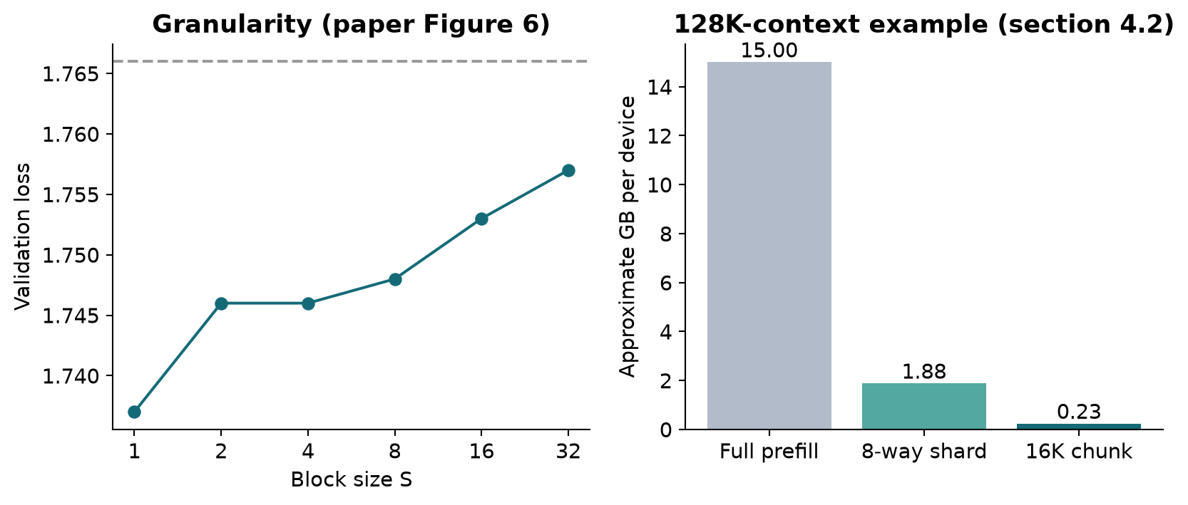
The block-size sweep gives losses 1.757, 1.753, 1.748, 1.746, and 1.746 for $S=32,16,8,4,2$, while Full at $S=1$ reaches 1.737. The plateau followed by an additional full-access gain is worth investigating: a simple monotone approximation story does not explain why $S=2$ and $S=4$ tie at reported precision. Optimization, interactions with the embedding source, or the particular sequence of layer types may matter.

Finally, the architecture sweep holds about $6.5\times10^{19}$ FLOPs and $2.3\times10^8$ active parameters fixed. The best tested width-to-depth ratio moves from about 60 to 45 under AttnRes. This suggests that the method can make extra depth useful in that regime. Deeper models also lengthen the sequential path at inference. A training-loss optimum is therefore an input to deployment design, not the final deployment objective.

10. A closer mathematical reading of gradients and matrix structure

The attention weights are helpful for visualization, but they are not the complete derivative of a layer input with respect to a source. Treat other sources as fixed and write $k_j=\operatorname{RMSNorm}(v_j)$. For the destination under consideration,

$$\frac{\partial\alpha_i}{\partial z_j} =\alpha_i(\mathbf1_{i=j}-\alpha_j).$$

Differentiate $h=\sum_i\alpha_i v_i$ with respect to the scalar score $z_j$:

$$\frac{\partial h}{\partial z_j} =\sum_i v_i\alpha_i(\mathbf1_{i=j}-\alpha_j) =\alpha_j(v_j-h).$$

The source also directly enters the value sum, while its key changes the logit. Applying the chain rule yields

$$\frac{\partial h}{\partial v_j} =\alpha_j I+ \alpha_j(v_j-h)\left(\nabla_{v_j}z_j\right)^\top.$$

This is a local partial derivative; the whole network additionally contains paths through later source construction. Even this local expression has a value term and a routing term. Thus, observing $\alpha_j\leq1$ does not imply a network gradient norm bounded by one, and a low attention weight does not by itself prove causal irrelevance. Normalization derivatives and query magnitude also matter.

For intuition, omit $\epsilon$ and learned channel scales temporarily. Let $r=\|v\|/\sqrt d$. Differentiating $v/r$ gives

$$J_{\rm norm}(v)=\frac1r\left(I-\frac{vv^\top}{\|v\|_2^2}\right).$$

The radial direction is removed, while tangential directions scale by $1/r$. This explains both why normalized keys ignore pure positive rescaling and why very small source norms require care. Actual RMSNorm retains $\epsilon$, so the exact derivative differs and remains regularized around zero. The displayed simplified derivative is an explanatory calculation, not a substitute for the full model definition.

The structured-matrix view needs similar care. The unrolled standard residual coefficients form a lower-triangular all-ones matrix with nonzero diagonal. Its ordinary matrix rank is $L$, despite its simple recurrent description. Its off-diagonal blocks across a depth cut have rank one. That latter property is the relevant semiseparable structure: a small recurrent state restricts how information can cross a cut through the computation.

A dense attention coefficient matrix can have richer off-diagonal structure, but saying that it has ordinary rank $L$ does not distinguish it from the standard residual matrix. Moreover, the coefficients are input dependent, and the source vectors themselves are constructed recursively. This is not one fixed linear operator describing the entire nonlinear network. I read section 6.2 as a useful representational analogy, while keeping ordinary rank, semiseparable rank, and the paper’s informal effective-rank discussion separate.

11. Limitations and experimental information still needed

The main evaluation establishes a promising result on a specific hybrid MoE family. It does not establish the same gains for dense decoders, every optimizer, post-training objectives, or arbitrarily deep models. The large model uses nine blocks rather than the approximate eight-block default of the scaling study. Hardware, context length, and training recipe belong to the result rather than being incidental details.

The benchmark table does not supply seed variation or confidence intervals. It also follows evaluation procedures from the Kimi Linear report rather than restating every decoding and prompting choice. A careful comparison should preserve those settings, benchmark versions, and scoring procedures. Where they are not specified in this report, the correct conclusion is that this document alone is insufficient to reconstruct the entire experiment.

The report’s latency claims lack a comprehensive workload matrix in the presented tables. Batch size, sequence length, precision, hardware, parallel layout, and the distinction between prefill and decode all affect the fraction of time consumed by residual operations. The under-2% inference figure is encouraging, but insufficient to predict a different production service’s tail latency or throughput.

Block compression still loses individual outputs. A fixed source budget trades representational detail for manageable state. Larger models can also have different distributions of source usefulness, so the success of roughly eight blocks should be tested rather than assumed. Learned boundaries or uneven block sizes could help, but would introduce their own scheduling and optimization costs.

The final limitation concerns interpretation. Token-averaged attention heatmaps hide variability across requests, tasks, and positions. Persistent embedding attention can indicate useful access to original features, a routing preference, or an attention sink. A heatmap alone cannot decide among these explanations. Intervening on a source and measuring the resulting loss is a stronger diagnostic than labeling large weights as the mechanism of improved reasoning.

12. Independent critical analysis and concrete next experiments

Separate normalized averaging from content selection. Zero-query initialization already changes the original sum into an average. A useful controlled study would compare standard residuals, a scale-matched fixed average, learned static mixtures, and content-dependent mixtures, with the same normalization placement and source storage. Matching the number of trained tokens is necessary, but matching optimization opportunities and scale is also relevant. This experiment could identify how much improvement comes from retrieval rather than a better-behaved magnitude trajectory.

Audit mathematical claims through definitions, not slogans. The $N=1$ endpoint, the $O(N^2)$ shorthand, and the use of rank in section 6.2 each require qualifications. These are presentation issues that affect how readers generalize the method. I would state the actual source sets, retain the $O(LNd)$ arithmetic expression, and define an off-diagonal rank measure before making capacity comparisons. This makes the theoretical picture testable without diminishing the empirical results.

Measure the block bottleneck directly. Full-versus-block validation loss is an aggregate outcome. A more informative diagnostic would measure cancellation within blocks, task-conditioned source importance, and the damage from replacing a selected block with zero or a matched-norm alternative. Compare fixed, layer-type-aligned, and learned boundaries under the same number of stored source vectors. If boundaries aligned with attention/MLP specialization recover a substantial fraction of the full-model gap, the result would suggest a practical improvement without increasing history capacity.

Evaluate a latency-quality frontier. The dynamic-query ablation has the lowest listed loss but worse scheduling properties. Rather than treating it as an abandoned variant, measure it alongside fixed-query Full and Block AttnRes under equal memory limits. Report prefill latency, decode latency, throughput at several batch sizes, and training time to a fixed validation target. The relevant winner may differ between offline training, interactive serving, and high-throughput batch inference.

Test whether distant access is causal. The sliding-window result motivates long-range depth retrieval, but does not identify which distant sources matter. Freeze a trained model, mask selected historical sources at evaluation, and compare against masks matched for total removed attention mass and source norm. Then retrain selected architectural variants to distinguish immediate dependence from adaptation. These are proposed experiments; this review has not performed model training or benchmark reproduction.

Use uncertainty where the comparison is close. At 241M, the displayed mHC(-lite) loss is 1.869 and Full AttnRes is 1.874; at other sizes the ordering changes. The general prose claim that Full always outperforms mHC is stronger than this table supports. Repeated runs at the close-comparison settings would be more informative than a single ranking. Likewise, the tie on MMLU-Pro should remain a tie, and rounding should not be interpreted as proof of identical underlying performance.

For readers planning a research comparison, I would first fix the mathematical architecture and source-count convention, then document the recipe and hardware. The most useful small checks are deterministic identities: softmax invariance to a common shift, exact merging of disjoint source sets, the absence of an empty partial source, and the relationship between transfer formulas and the assumed schedule. Those checks establish the explanation’s internal consistency. They do not substitute for training evidence.

13. Conclusion

Attention Residuals makes a familiar operation newly explicit: combining earlier representations is a modeling choice. Full AttnRes grants token-dependent access to individual layer outputs; Block AttnRes keeps a smaller set of summaries; fixed pseudo-queries enable a schedule that reuses completed-history work. The systems contribution is integral to the method because activation traffic and pipeline communication otherwise threaten the appeal of a parameter-light modification.

My main takeaway is the joint design of representation and access. Summaries determine what a later layer can recover, while scheduling determines how expensive that access becomes. The paper offers credible evidence that this trade-off can improve its tested model family. The next step is to characterize where the gains come from, how uncertainty affects close comparisons, and which point on the quality-latency frontier remains attractive under different workloads.

References and provenance

• Kimi Team. Attention Residuals, arXiv:2603.15031v1, 2026-03-16. Equations, experimental values, and the reported systems accounting in this review refer to this version; Appendix A gives the full authorship and contribution order, and Appendix B derives Full AttnRes I/O.
• Official project resource, linked from the paper.
• All nine figures here are original explanatory diagrams or redrawings of explicitly identified numerical facts. Hypothetical vectors, source counts, and analytical memory calculations are labeled as such. The paper is distributed under CC BY-NC-ND 4.0; no original paper figure is reproduced or edited here.
• Mathematical examples and arithmetic in this review are independent explanatory calculations. No model-training run, author experiment, or production latency result is claimed as independently reproduced.