QeRL: When Quantized Weights Help Reinforcement Learning, and Where the Evidence Stops

Review date: 2026-09-17. Author: Zhongzhu Zhou.

Paper reviewed: QeRL: Beyond Efficiency — Quantization-enhanced Reinforcement Learning for LLMs.

Paper authors: Wei Huang, Yi Ge, Shuai Yang, Yicheng Xiao, Huizi Mao, Yujun Lin, Hanrong Ye, Sifei Liu, Ka Chun Cheung, Hongxu Yin, Yao Lu, Xiaojuan Qi, Song Han, Yukang Chen.

arXiv: 2510.11696v1, submitted 2025-10-13, 21 pages. Numerical references below refer specifically to the arXiv v1 PDF, not an assumed identical proceedings revision.

1. What I think the paper contributes

QeRL connects two constraints that are usually discussed separately. A reinforcement-learning policy must fit in memory while generating many candidate responses; it must also explore enough useful responses to receive a learning signal. The paper uses a frozen NVFP4 backbone with trainable low-rank adapters, and proposes scheduled perturbations of normalization scales to improve exploration. Its interesting claim is that compressed representations can change the optimization trajectory beneficially, rather than merely recover the quality lost by compression.

I separate that claim into three questions. First, does the representation reduce storage and accelerate the relevant kernels? Second, does the altered policy generate better learning data? Third, does the combined method reduce time to a chosen evaluation target? Evidence for one question does not automatically answer the others. A faster decoder can still sit inside a slower training loop, and higher token entropy can describe either productive exploration or incoherent output.

The main results make QeRL worth studying. In the paper’s 7B GSM8K experiment, NVFP4 with AQN reaches 90.8%, versus 88.1% for BF16 LoRA and 91.2% for full fine-tuning. The wider benchmark table is more mixed: for 7B, adding AQN to NVFP4 LoRA reduces the four-task mean from 37.0 to 36.4, even while improving MATH500. The framework also demonstrates a constrained 32B training configuration on an H100 80GB. These are useful observations, but they do not establish uniform superiority over BF16, or a universal relationship between quantization and reasoning.

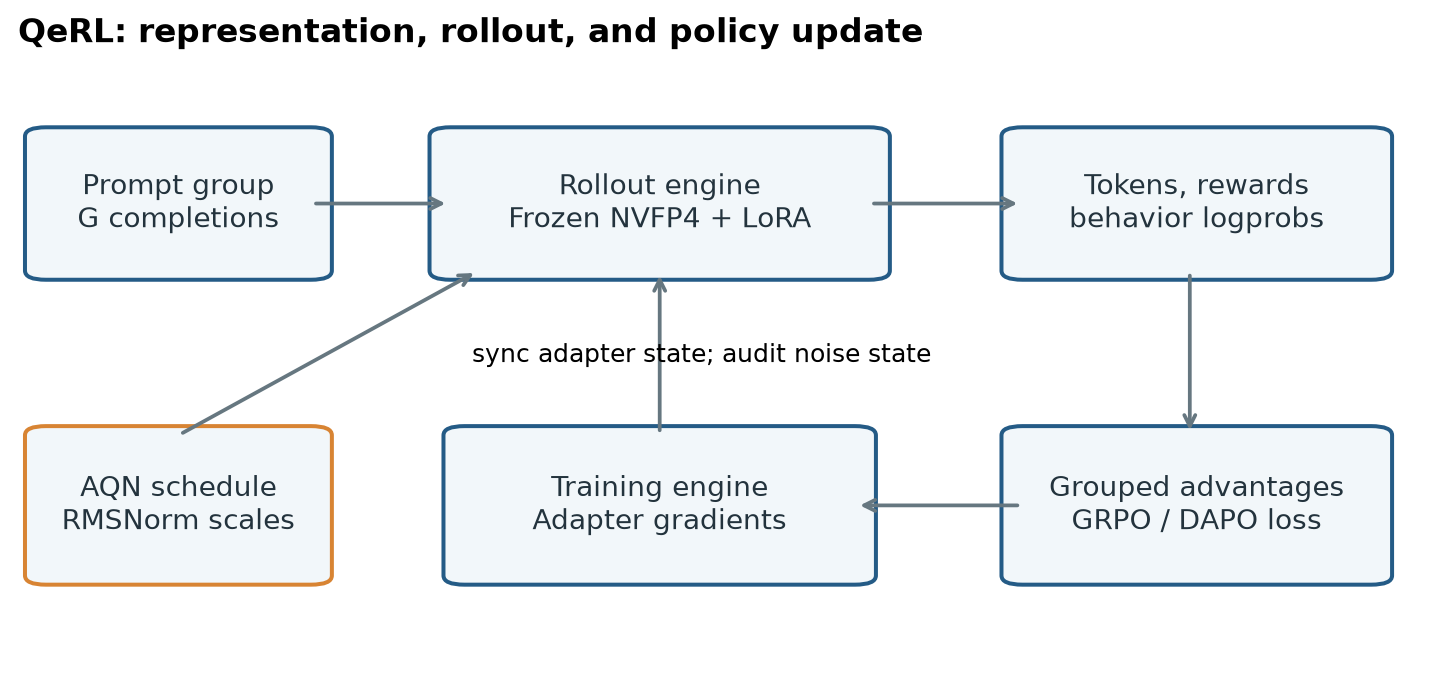
The diagram places behavior log-probabilities beside generated tokens deliberately. Once a noise draw changes the sampling policy, the probabilities used to explain those samples are part of the experiment. A reader who only follows the packed weights and adapter matrices can miss the most consequential statistical question in the implementation.

2. Prerequisites: the quantities that actually change

2.1 Weight storage and trainable state are different budgets

Let a projection use column-vector notation with $W\in\mathbb{R}^{d_o\times d_i}$. LoRA replaces a full update by $BA$, where $A\in\mathbb{R}^{r\times d_i}$ and $B\in\mathbb{R}^{d_o\times r}$. With an explicit adapter multiplier $\lambda$, the forward map is

$$y=\widehat W x+\lambda B(Ax),\qquad \widehat W=Q(W).$$

The backbone is frozen; gradients update $A$ and $B$. Freezing removes its optimizer state and parameter gradients, but not its forward multiplication. Nor does it remove all backward computation: gradients may need to pass through a frozen projection to reach an earlier adapter. The model still processes every relevant token. This explains why LoRA can save much more memory than elapsed time.

A square $4096\times4096$ matrix contains 16,777,216 weights. Rank 32 adds $32(4096+4096)=262,144$ adapter parameters, or 1.5625% of that matrix’s count. This is an illustrative layer calculation, not the parameter fraction measured for the complete QeRL models. Different projection dimensions, embeddings, and trainable normalization parameters change the model-wide fraction.

For a row batch $X$, I will switch explicitly to $W\in\mathbb{R}^{d_i\times d_o}$ in the normalization derivation. That convention lets input-channel modulation appear as row scaling. The transpose is bookkeeping; confusing the conventions is how a vector-shaped noise term starts being treated as an arbitrary weight matrix.

2.2 Why a group reward supplies an advantage

For a prompt $q$, sample $G$ responses and evaluate scalar rewards $R_1,\ldots,R_G$. A group-relative advantage is

$$\bar R=\frac1G\sum_{i=1}^G R_i,\qquad s_R=\sqrt{\frac1G\sum_{i=1}^G(R_i-\bar R)^2},\qquad A_i=\frac{R_i-\bar R}{s_R+\epsilon}.$$

The subtraction asks whether a response is better than its peers. The division changes the weighting of prompt groups, so it is not merely a harmless numerical convention. The small $\epsilon$ handles a zero denominator, but an all-equal reward group still has zero numerator and provides no reward-driven update. Dynamic sampling can address the frequency of uninformative groups; it does not make bad responses informative by definition.

For binary rewards $[1,0,0,0]$, the mean is $1/4$, the population standard deviation is $\sqrt3/4$, and the advantages without numerical epsilon are $[\sqrt3,-1/\sqrt3,-1/\sqrt3,-1/\sqrt3]$. For $[0,0,0,0]$, every advantage is zero. Exploration is useful when it turns some previously uniform groups into discriminative ones. This is a more operational hypothesis than merely increasing entropy.

GRPO’s characteristic economy is removing the learned value critic. It does not logically forbid a learned reward model. QeRL uses mathematical reward tasks; this particular reward design should not be generalized into a definition of GRPO. Similarly, its introductory KL-regularized equation is not the exact configuration of every experiment: Appendix E states that the reported training uses neither entropy nor KL losses.

2.3 Policy ratios need a precisely defined behavior policy

Write the token state as $s_{i,t}=(q,o_{i,<t})$. If $\pi_b$ generated the response, a usual token ratio is

$$\rho_{i,t}(\theta)=\exp\!\left[\log\pi_\theta(o_{i,t}\mid s_{i,t})-\log\pi_b(o_{i,t}\mid s_{i,t})\right].$$

The clipped surrogate uses the smaller of $\rho A$ and a clipped-ratio version. Positive advantages stop benefiting from excessively large ratios; negative advantages impose the opposite one-sided constraint. Clipping limits the surrogate’s incentive to change already distant probabilities. It cannot repair a denominator computed by a different stochastic model from the one that sampled the token.

The distinction matters for QeRL because the base quantization is fixed while AQN changes another part of the policy. Equal bit-widths across training and rollout do not guarantee equal distributions. Adapter versions, noise draws, normalization state, temperature, top-p truncation, and numerical kernels also matter. I would record each of these before interpreting a training ratio near one as evidence of on-policy data.

3. NVFP4: a storage format with a kernel contract

3.1 What the four bits represent

FP4 E2M1 has one sign bit, two exponent bits, and one mantissa bit. Its nonnegative values include $0,0.5,1,1.5,2,3,4,6$; this is not a uniformly spaced integer grid. NVFP4 combines those values with one FP8 E4M3 scale for each block of 16 weights and a global FP32 scale. For weight $j$ in block $b$, reconstruction is

$$\widehat w_{b,j}=s_g s_b q_{b,j},\qquad q_{b,j}\in\mathcal F_{\mathrm{E2M1}}.$$

For fixed scales, a conceptual nearest-grid quantizer selects

$$q_{b,j}=\arg\min_{q\in\mathcal F_{\mathrm{E2M1}}}|w_{b,j}-s_gs_bq|.$$

This expression explains reconstruction, not the complete AWQ calibration procedure. Choosing clipping and scales to minimize activation-weighted error can produce a different answer from independently minimizing each weight’s error. QeRL calibrates its FP4 formats using an AWQ procedure with 256 sequences of length 2048 from OpenThoughts-114k. NF4 uses its default configuration in the reported comparison. Therefore, the experiment changes calibration methodology as well as representation and kernel support.

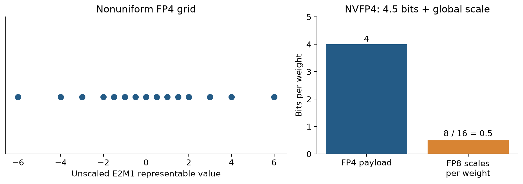
A simple memory derivation is useful. For $P$ quantized weights, ignoring padding and the small number of tensor-global scales,

$$M_{\mathrm{NVFP4}}\approx \frac{4P}{8}+\frac{8(P/16)}8 =\frac{9P}{16}\text{ bytes}.$$

BF16 needs $2P$ bytes, so the ideal ratio is $2/(9/16)=32/9\approx3.56$. Calling NVFP4 a guaranteed fourfold reduction loses the scale metadata. Calling that ratio a training-memory reduction loses activations, KV cache, adapters, optimizer state, workspaces, and duplicated engine state. The NVIDIA format description confirms the 4.5-bit accounting.

3.2 Why low precision can still be slower

During autoregressive decoding, one token often reuses a large weight matrix with little arithmetic per fetched byte. Packed weights can reduce bandwidth pressure. But the GPU must unpack codes, apply scales, and feed a supported multiply instruction. A poor conversion path can spend more time decoding the representation than it saves moving bytes. QLoRA’s low storage footprint therefore does not itself predict rollout throughput.

QeRL uses a Marlin NVFP4-by-BF16 path. It is essential to distinguish software support for NVFP4 weight storage on Hopper from native FP4 Tensor Core arithmetic. H100 results in this paper do not demonstrate native Blackwell FP4 instructions on H100. The model format, arithmetic used after unpacking, accumulator precision, and target architecture are four separate implementation choices.

The frozen backbone is helpful here. If every training step changed the dense base weights, a packed layout and calibrated scales would need frequent rebuilding. LoRA keeps the packed backbone stable and adds a small higher-precision update. The alternative is full quantization-aware training with trainable base parameters, but then gradient representation, rounding policy, and scale updates become a different research problem.

Algorithm 1: preparing a QeRL-style backbone. These are explanatory steps derived from the paper, not a replacement for the repository’s exact packing code.

1. Freeze the chosen pretrained checkpoint and record its tokenizer and chat template.
2. Select representative calibration sequences; record their origin and lengths.
3. Calibrate block scales and any activation-aware transforms for the selected weight matrices.
4. Quantize values to E2M1 codes; retain block E4M3 scales and tensor-global scales.
5. Pack codes into the layout required by the chosen inference kernel.
6. Attach LoRA adapters to the selected projections; record rank and scaling convention.
7. Compare dequantized reference outputs with the packed kernel on fixed inputs.
8. Measure both model footprint and complete engine peak allocation before starting RL.

Step 7 should precede rewards and sampling. If a layout mistake changes matrix semantics, an RL run may partially adapt around it and conceal the original defect. A fixed-input projection check is cheap and much easier to diagnose.

4. Quantization noise does not automatically increase entropy

4.1 A local derivation makes the missing condition visible

The fixed quantization residual is $E=\widehat W-W$. For a given prompt, it perturbs the model’s logits by some $\delta z$. Even if weight errors were unbiased under a calibration distribution, the induced logit change for a particular prompt need not be unbiased. A multilayer nonlinear network does not preserve that property automatically.

Let $p_i=\exp(z_i)/\sum_j\exp(z_j)$ and $H(p)=-\sum_i p_i\log p_i$. First differentiate softmax:

$$\frac{\partial p_i}{\partial z_j}=p_i(\mathbf1_{i=j}-p_j).$$

Then apply the chain rule to entropy. The derivative of $-p_i\log p_i$ is $-(\log p_i+1)\,dp_i$, and the probability derivatives sum to zero. Substituting yields

$$\frac{\partial H}{\partial z_j} =-p_j(\log p_j+H).$$

Consequently the first-order entropy change is

$$\Delta H\approx-\sum_j p_j(\log p_j+H)\delta z_j.$$

Nothing fixes its sign. Raising an already dominant logit usually makes the distribution sharper; lowering it may flatten the distribution. The paper’s entropy curves are evidence about its models and training conditions, not a theorem that every quantizer promotes exploration.

For a concrete deterministic check, take logits $(2,0,-1)$. Their entropy is approximately 0.524 nats. Adding $0.5$ only to the largest logit reduces entropy to about 0.386; subtracting $0.5$ increases it to about 0.680. These are illustrative softmax calculations made for this review. They are not measurements on Qwen. A finite-difference check of the derivative accompanies the figure.

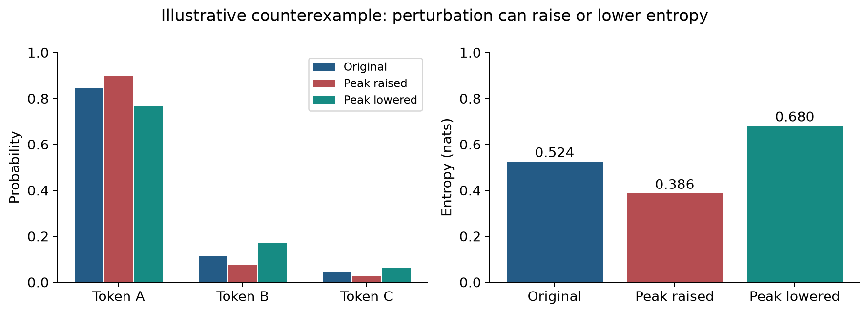
Even zero-mean stochastic perturbation does not settle the question. Expanding around the unperturbed logits, with covariance $\Sigma$, gives

$$\mathbb E[\Delta H]\approx \frac12\operatorname{tr}\!\left(\nabla_z^2 H\,\Sigma\right).$$

The first-order term cancels under the stated zero-mean assumption; the remaining term depends on curvature and covariance. At a uniform distribution entropy is already maximal, so a nontrivial perturbation that makes each realization nonuniform cannot increase the average entropy of individual realizations. This simple boundary case refutes an unconditional claim while leaving the paper’s empirical result entirely possible.

4.2 Diversity between policies differs from entropy within a policy

If a random noise state $Z$ is sampled, there are two quantities worth measuring: the entropy of the mixture policy and the average entropy conditional on the draw. With $O$ denoting a token or response at a fixed prompt,

$$H(O\mid q)=\mathbb E_Z[H(O\mid Z,q)]+I(O;Z\mid q).$$

The mutual information term measures how strongly different noise states change the output. A mixture can be diverse because each noise state selects a different confident response, even though every conditional policy has low entropy. This can be useful coherent exploration. Conversely, injecting fresh noise independently at each decoding step may increase local uncertainty without maintaining a consistent strategy over the response.

For this reason, I would measure noise persistence over tokens and responses alongside entropy. I would also report the fraction of reward groups with both successes and failures, unique valid solution paths, answer-format failures, and reward conditioned on response length. These diagnostics connect exploration to learning opportunities. Token entropy alone leaves the connection implicit.

5. AQN and the exact meaning of noise sharing

5.1 Deriving the RMSNorm identity

Use row-vector notation now. Let $u=x/\sqrt{d^{-1}\sum_jx_j^2+\delta}$ be a normalized activation and let $w$ be the channel-wise RMSNorm scale. The ordinary output before a projection is $h=u\odot w$. Adding a noise vector $z$ to the scale gives

$$h_z=u\odot(w+z)=u\odot w+u\odot z.$$

If every $w_j\ne0$, define $d_j=1+z_j/w_j$. Then $h_z=h\odot d$, and for a projection $W\in\mathbb R^{d_i\times d_o}$,

$$h_zW=h\operatorname{diag}(d)W =h\left[\operatorname{diag}(1+z/w)W\right].$$

Thus additive noise on normalization scales corresponds to multiplicative row modulation of the following matrix. It does not correspond to a general additive matrix $W+Z$ with independently chosen entries. The paper’s broad additive-noise motivation and its efficient implementation should be kept distinct. The normalization implementation provides a structured, low-dimensional family of perturbations.

The nonzero-scale condition only belongs to the equivalent ratio representation. The direct expression $u\odot(w+z)$ remains defined when a scale is zero. Near-zero scales are nevertheless relevant: a small absolute $z_j$ can be large relative to $w_j$, making the apparent relative weight perturbation large. A robust implementation can monitor relative perturbation statistics without explicitly dividing by tiny scales in the forward computation.

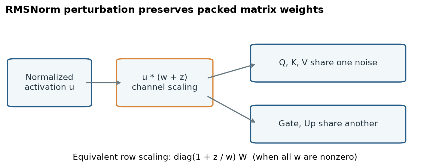
The shared scale preserves the packed matrix kernel because the activation has already been rescaled by normalization. No new dense weight matrix is required. However, zero added trainable parameters is not literally zero execution cost: random-number generation, synchronization, state restoration, and cache invalidation still have to occur somewhere. Their cost may be small, but it should be measured rather than removed from the accounting by terminology.

Q, K, and V share the same normalized input, so their perturbations are correlated. Gate and Up share another input in a gated feedforward block. Down occurs after gating and multiplication and is not directly adjacent to that pre-FFN normalization. Appendix G’s sentence referring to Down and Up sharing noise does not match the architecture drawn in Figure 6 or the main text, which names Gate and Up. I follow the computational graph in the derivation.

5.2 A schedule needs consistent endpoints

The paper motivates a zero-extra-noise warm-up followed by decreasing stochastic noise. A precise ten-stage convention is to use stage 0 for warm-up and stages 1 through 9 for positive scales:

$$\sigma_0=0,\qquad \sigma_k=\sigma_{\mathrm{start}} \left(\frac{\sigma_{\mathrm{end}}}{\sigma_{\mathrm{start}}}\right)^{(k-1)/8}, \quad k=1,\ldots,9.$$

With start 0.01 and end 0.0005, stage 1 is exactly the start and stage 9 exactly the end. The logarithm changes linearly with stage, so successive nonzero scales have a constant ratio. This gives relatively fast early reduction followed by smaller absolute changes. It is a manually selected annealing schedule, not feedback control based on measured reward or entropy.

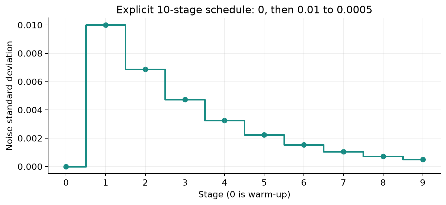
The v1 text mixes stage conventions: Equation 8’s positive stages and Algorithm 1’s zero-based warm-up require an explicit indexing convention. The formulation above uses nine positive levels for ten total stages and a denominator of eight so that both endpoints are attained. This is an interpretation of the paper’s schedule, not a claim about a particular software execution.

The paper also presents more than one numerical range: the main text mentions 0.05 to 0.0005, while Table 4 states 0.01 to 0.0005. Comparisons should identify which paper setting they use instead of treating the two ranges as interchangeable.

6. A training algorithm that exposes the stochastic state

I find it useful to rewrite the training loop with the behavior policy made explicit. The following explanatory specification brings together the paper’s equations and prose. It is not a claim that every listed step was documented in the original experiments.

Algorithm 2: an explicit rollout-and-update cycle.

1. Load frozen quantized weights, adapter state, normalization scales, tokenizer, and generation configuration.
2. Determine the current schedule stage from the number of completed updates and the planned horizon.
3. Snapshot clean normalization scales and identify the exact modules eligible for perturbation.
4. Draw a noise state using a recorded seed and a declared persistence scope: per rollout, per response, or per token.
5. Construct the behavior policy from the adapter version, perturbed scales, temperature, and support restriction.
6. Generate a response group for each prompt; retain token masks and the probabilities required by the chosen estimator.
7. Compute rewards and grouped advantages; distinguish valid failures, parser failures, and truncations.
8. Restore clean scales or replay the intended noise state for training, according to the explicitly chosen objective.
9. Compute policy ratios against the actual behavior-policy denominator and apply the selected clipped loss.
10. Update trainable parameters, synchronize the rollout engine, and invalidate any cached values tied to old parameters.
11. Log valid-group fraction, length, entropy definition, ratio statistics, peak memory, and time per stage.
12. Evaluate a declared deployment policy, including whether AQN is disabled, using fixed evaluation settings.

The key choice is step 8. One objective trains a conditional noisy policy, treating $Z$ as part of the sampled context. Another trains a clean deployment policy from noisy behavior trajectories. These are different estimators. Both can be made principled, but the bookkeeping must match the intended target.

For a noise draw per response, write the conditional behavior distribution as

$$P_b(o\mid q,z)=\prod_t\pi_b(o_t\mid q,o_{<t},z).$$

Its marginal over noise is an expectation of a product:

$$P_b(o\mid q)=\mathbb E_Z\left[\prod_t\pi_b(o_t\mid q,o_{<t},Z)\right].$$

This is generally not the product of independently noise-averaged token probabilities. A retained noise draw supplies a tractable conditional probability, but the learning objective then needs to recognize that conditioning. If targeting a clean policy with exact trajectory importance sampling, the product of ratios can have high variance. GRPO’s clipped token surrogate is already an approximation to that broader off-policy problem; additional untracked noise should not be described as automatically corrected by matching weight precision.

There is a second support issue. Top-p sampling can remove tokens with positive probability under the clean policy. An importance ratio cannot recover clean-policy probability mass that has zero behavior support. Temperature changes also affect the actual sampling distribution. These are familiar practical compromises in LLM RL, not problems unique to QeRL, but AQN makes it more important to state the chosen convention. An experiment report should state whether probabilities correspond to raw model logits or the transformed sampler.

7. Reading the experimental results without flattening them

7.1 Accuracy gains depend on the dataset and comparison

The paper’s Table 1 uses GRPO and GSM8K; Table 2 uses DAPO and BigMath training followed by four benchmark evaluations. They should not be treated as the same training run. Here are selected values copied from those tables, with no averaging across incompatible protocols.

Setting	BF16 LoRA	NVFP4 LoRA	NVFP4 + AQN	BF16 Full
GSM8K, 3B	76.1	83.3	83.7	84.4
GSM8K, 7B	88.1	88.5	90.8	91.2
Mean, 7B	35.7	37.0	36.4	37.3
Mean, 14B	40.2	40.5	42.0	43.3
Mean, 32B	42.2	41.4	45.6	46.2

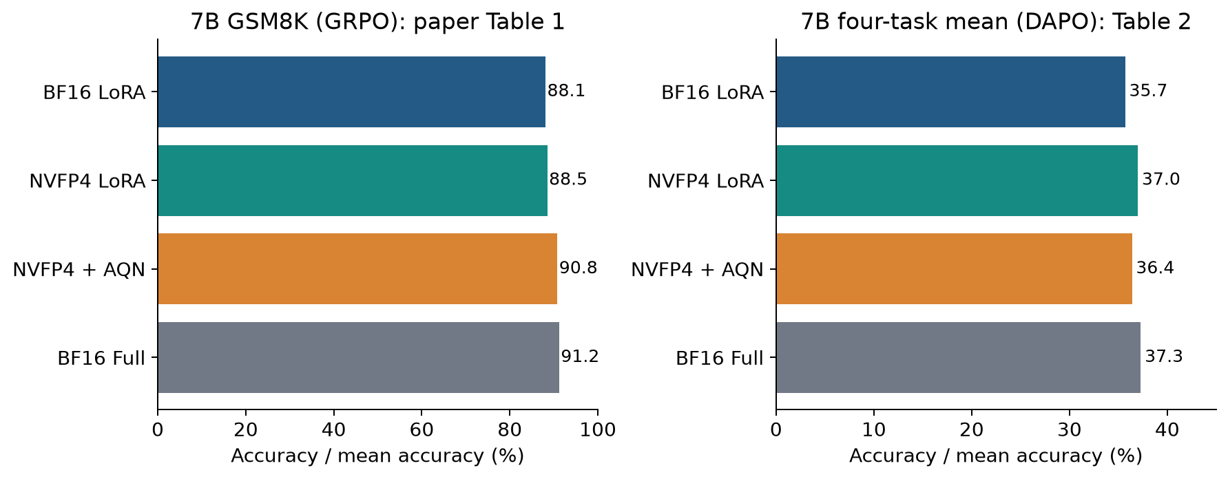
The GSM8K difference between 90.8 and 88.1 is 2.7 percentage points. Section 4.2 says 1.7 points; the table arithmetic supports 2.7. This discrepancy is small in scope but illustrates why I use raw table cells as the traceable record rather than repeating prose summaries.

For 7B in Table 2, AQN changes MATH500 from 76.8 to 77.4, AIME24 from 13.7 to 15.5, leaves AIME25 at 10.0, and changes AMC23 from 47.5 to 42.5. The arithmetic mean therefore falls by roughly 0.6 points. AQN can help some evaluation distributions while harming others. A useful follow-up would examine whether the changing training distribution, response length, or noise schedule predicts which tasks benefit.

The comparison with full fine-tuning is likewise conditional. QeRL matches the reported 7B MATH500 score of 77.4, but trails the full-update mean in the selected 7B, 14B, and 32B rows. A feasible compressed run with close quality is a meaningful achievement without requiring equality on every benchmark. Reporting the whole vector avoids hiding that distinction.

7.2 Learning rate is part of the treatment

Appendix E sets a learning rate of $10^{-5}$ for the quantized variants and $5\times10^{-6}$ for BF16 LoRA, explaining that larger BF16 updates can collapse. Appendix I compares larger rates and shows different stability behavior. This is evidence that the useful training recipe changes with the representation. It is not a clean experiment in which only numerical noise changes.

There are two legitimate comparisons. A controlled-mechanism study holds learning rate, data order, group size, and optimizer schedule fixed to test the effect of quantization or AQN. A practical best-recipe study tunes each method with equal search budgets and compares the best robust result. The paper contains evidence relevant to both but does not fully disentangle them. Claiming that all faster reward growth is caused by entropy would skip this confound.

The main rank reported in the paper is 32. The paper’s rank ablation suggests similar reward trends in one setup; it does not guarantee rank independence across models and data. A rank sweep also changes adapter kernel overhead and the subspace in which the policy can compensate for quantization errors. I would include both quality and throughput in that sweep.

8. Systems accounting: from a smaller model to a faster run

8.1 Model footprint is only one memory component

Tables 5 through 8 report model sizes of 6.2/2.8 GB, 15.2/5.9 GB, 29.6/10.6 GB, and 62.3/20.7 GB for BF16/NVFP4 at 3B, 7B, 14B, and 32B. I keep the paper’s GB label rather than assuming a binary-unit conversion. These reported values do not equal the ideal scale-only bound, because not every parameter and allocation follows the same packing rule.

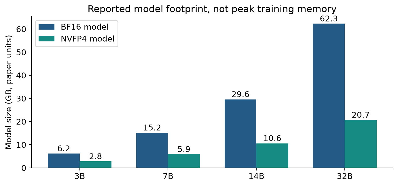
An operational peak budget is closer to

$$M_{\mathrm{peak}}=M_{\mathrm{resident\ weights}}+M_{\mathrm{adapters/state}} +M_{\mathrm{activations}}+M_{\mathrm{KV}}+M_{\mathrm{workspace}}+M_{\mathrm{reserve}}.$$

The first term must count actual copies rather than assuming one logical model means one allocation. Reference-policy evaluation, colocated inference engines, and synchronization buffers can all matter. Weight compression frees budget that may be reinvested into KV cache and longer sequences; if the engine reserves a fixed fraction of GPU memory, observed allocation may not fall by the weight ratio.

Gradient checkpointing trades extra computation for smaller saved activations. It can turn an out-of-memory configuration into a runnable one; that is not the same as making a previously runnable identical configuration faster. For 32B, Table 8 reports BF16 LoRA out of memory and QeRL with checkpointing completing steps. The correct conclusion is feasibility under those settings, not an unbounded numerical speedup relative to the failed run.

8.2 A speedup requires an explicit denominator

For batch size 2, dividing QeRL rollout throughput by BF16 LoRA throughput in Tables 5 through 8 gives approximately 1.04, 1.31, 1.46, and 1.76 for 3B through 32B. These are independently recomputed ratios of reported numbers, not new performance measurements. Table 7 prints 1.3 for the 95.3/65.4 row, although the quotient is approximately 1.46. Figure 11’s roughly twofold annotations use the slower QLoRA denominator; they should not be relabeled as twofold gains over vanilla LoRA.

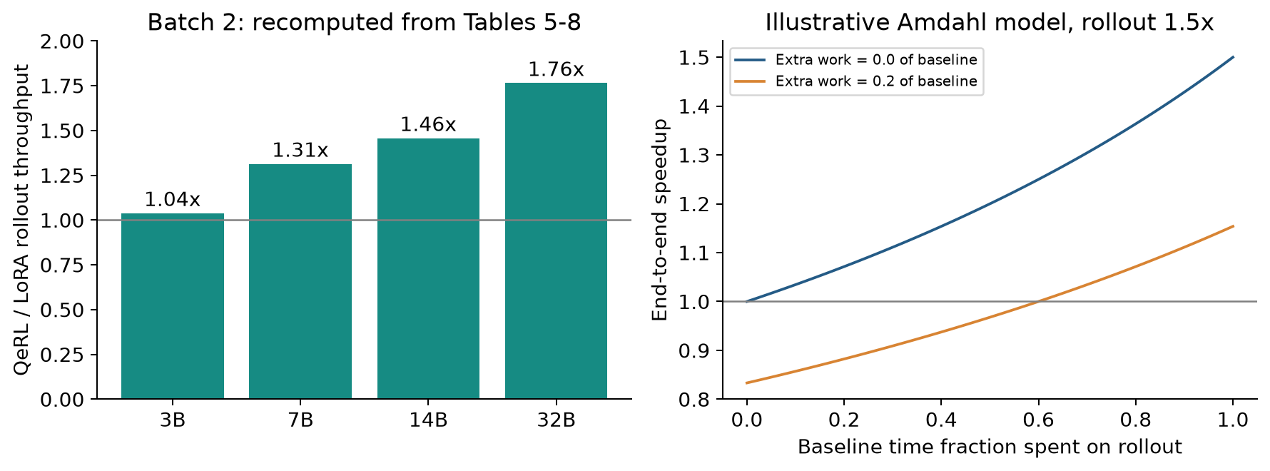
Let a baseline step take $T$, and let rollout occupy fraction $f$. Suppose rollout becomes $s$ times faster, while new overhead costs $\eta T$. Then

$$T'=T\left[(1-f)+\frac f s+\eta\right],\qquad S_{\mathrm{E2E}}=\frac1{(1-f)+f/s+\eta}.$$

For $f=0.7$, $s=1.5$, and $\eta=0$, the total speedup is about 1.30. Add overhead of $0.2T$ and it falls to about 1.03. If only 40% of the baseline is rollout, the same overhead makes the combined method slower, about 0.94x. The break-even condition is $\eta<f(1-1/s)$.

Gradient accumulation can also change the balance between rollout and training computation. More log-probability and backward work can reduce the effect of a faster decoder on total elapsed time. Measurements should report generation, probability evaluation, backward, optimizer, and synchronization costs under the same token workload.

9. Noise semantics and controlled experiments

9.1 Replacing noise and accumulating noise are different processes

A decaying noise schedule describes the size of each draw. It does not, by itself, specify the total displacement of the policy. Two elementary stochastic processes illustrate why that distinction matters when interpreting the method.

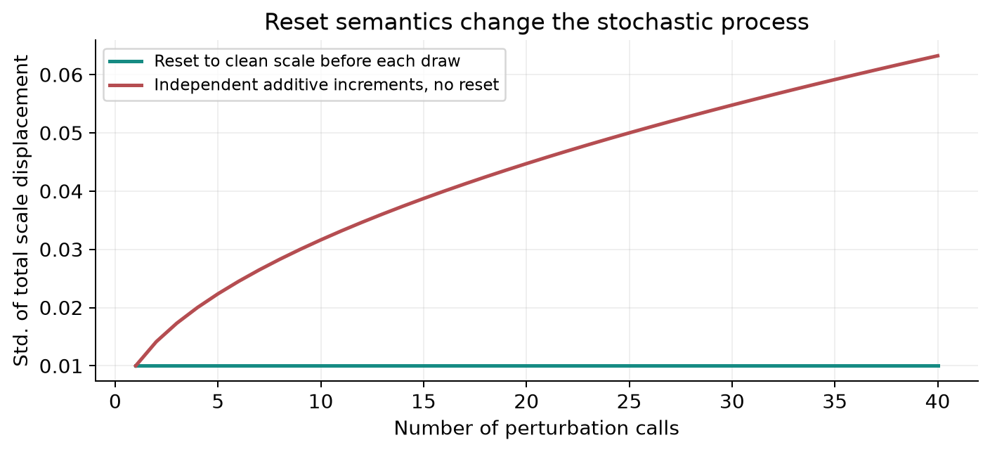
If the clean scale is restored before each draw, displacement variance is simply $\sigma_k^2$. If it is not restored and increments are independent, then after $K$ calls,

$$w_K-w_0=\sum_{k=1}^K z_k,\qquad \operatorname{Var}(w_K-w_0)=\sum_{k=1}^K\sigma_k^2.$$

A decreasing increment size does not make cumulative displacement shrink. A description of the stochastic process must therefore state whether each draw replaces the preceding perturbation or adds to it. The same equation also shows why schedule plots alone cannot demonstrate that actual parameter noise anneals toward zero.

9.2 An experiment matrix that separates explanations

A useful first replication would compare BF16 LoRA, BF16 LoRA with matched RMSNorm noise, NVFP4 LoRA without AQN, and NVFP4 LoRA with AQN. Add a temperature-adjusted BF16 baseline matched approximately on initial entropy. This isolates whether structured parameter-space perturbation offers something beyond a hotter sampler and whether the noise benefit depends on the quantized backbone.

For each method, use both a common learning-rate grid and an equal-budget per-method tuning protocol. Keep reward extraction, prompt data, truncation handling, and evaluation policy fixed. Report several independent training seeds and repeated evaluation samples where appropriate. Benchmark-specific uncertainty is more informative than a single mean across tests of different sizes.

I would measure time to a prespecified held-out reward or accuracy target, total generated tokens, GPU-hours, and peak allocated and reserved memory. Quality should be measured under the intended deployment policy with explicitly stated AQN handling. If a run never reaches the target within budget, record it as censored or unsuccessful at that budget rather than extrapolating a convergence time.

9.3 What was verified in this review

The deterministic checks verify the normalization identity on 50 random matrix cases, with maximum absolute discrepancy approximately $3.6\times10^{-15}$ in float64 arithmetic. The entropy derivative matches a central finite difference to approximately $8\times10^{-12}$. The schedule endpoints and table ratios were calculated directly. Nine static explanatory or data-redrawn figures are embedded in the document.

These checks support the algebra and arithmetic used here; they are not a reproduction of the training results. The analysis draws on the complete arXiv v1 paper, NVIDIA’s format documentation, and the conference listing.

10. Limitations of the demonstrated result

The empirical scope is mathematical reasoning, primarily Qwen2.5-Instruct models from 3B to 32B. The paper does not establish transfer to code-generation RL, tool-using agents, broad language quality, or much larger and mixture-of-experts models. Its training mechanisms might transfer, but both reward informativeness and sensitivity to noise can change with those settings.

There is no broad multi-seed uncertainty analysis in the reported tables sufficient to support a claim that every small numerical difference is reliable. Evaluation repeats are mentioned, but they should not be confused with independent training seeds. Differences on small benchmark sets are particularly difficult to interpret without per-example outcomes and confidence intervals.

The single-H100 claim concerns specific efficiency settings. Section 4.1 says the final evaluated models were trained using eight H100 GPUs for experimental efficiency. Thus the paper does not establish that all headline accuracy numbers were obtained through the demonstrated single-GPU recipe. These two experiments answer related but distinct questions: whether a configuration fits and whether a training approach reaches strong quality.

Finally, model-size tables do not fully characterize peak memory, and early-step averages do not characterize every point in a run whose response lengths evolve. The main and appendix efficiency tables use overlapping but nonidentical presentations. Their discrepancies should motivate publication of machine-readable benchmark manifests and raw timings, rather than selection of the largest multiplier.

11. Independent critical analysis

11.1 The causal explanation needs a stronger intervention

The strongest interpretive gap is between observing higher entropy and concluding that quantization causes useful exploration that causes faster learning. Quantization also changes initial accuracy, calibration error, activation geometry, stable learning rates, and the correction burden on the adapter. Each can affect the reward curve. Matching only entropy would not match all those factors, but a carefully designed intervention can establish whether entropy is a mediator rather than a correlated symptom.

My preferred intervention holds the backbone fixed and changes one source of randomness at a time. Compare deterministic quantization, repeated stochastic scale changes, and output-temperature changes; measure valid-group probability and held-out quality. If only structured perturbation helps at matched entropy, the mechanism is richer than distribution flattening. If temperature captures the gain, the cheaper control deserves consideration.

11.2 The mathematical abstraction should reflect the deployed perturbation

A shared channel-scale vector is attractive because it respects a fast packed kernel. Its perturbation family is much narrower than independent matrix noise, and it couples Q/K/V and Gate/Up. That structure may be the reason it works, rather than an implementation detail to be hidden behind a general additive-noise equation. I would explicitly parameterize the covariance induced on each projection and compare independent versus shared noise at the same output-perturbation budget.

A practical extension is layer-sensitive noise. One can scale perturbations by normalization-weight magnitude or by a measured logit sensitivity, then cap the change to avoid a few channels dominating. This is a proposed experiment, not an improvement established by this review. It should be evaluated against the simpler global schedule with equal tuning cost, because extra hyperparameters can easily erase a claimed efficiency advantage.

11.3 The right systems objective is useful learning per budget

I would evaluate a Pareto frontier over held-out quality, elapsed time, and peak memory. In some regions, QeRL may make an otherwise impossible experiment possible; in others, BF16 LoRA may remain faster because logits and backward dominate. A method can be valuable in the first region even if it loses the second. The practical conclusion should name the region, model size, and workload rather than assign a universal speedup.

A more ambitious controller could adapt noise using the fraction of informative reward groups, while keeping entropy and invalid-output rate within a target band. Such a controller would finally make adaptation responsive to the actual learning process. It would also require stability checks and an ablation against the fixed schedule. I would start by logging those signals before introducing the controller.

12. Conclusion

My reading is that QeRL provides a credible recipe for combining compressed frozen weights, inexpensive policy updates, and structured exploration. Its most persuasive result is a useful quality-and-resource tradeoff in the tested mathematical RL settings. The recipe is especially interesting when weight residency and autoregressive rollout are major bottlenecks.

The paper does not show that quantization always increases entropy, that AQN improves every task, or that every end-to-end run is twice as fast as BF16 LoRA. The algebra and table arithmetic explain where those stronger interpretations fail. For an actual deployment, I would first establish noise semantics and likelihood consistency, then compare time to target quality under a measured memory budget. That sequence tests the distinctive promise of QeRL while preserving a clear explanation of what caused the gain.

Sources

1. Huang et al. QeRL, arXiv v1. Primary method, Tables 1-9, Appendix E-K. The paper is distributed under CC BY 4.0; all figures here are original explanations or labeled redraws.
2. NVIDIA, Introducing NVFP4 for Efficient and Accurate Low-Precision Inference, 2025-06-24. Format and scale accounting.
3. ICLR 2026 conference record. Venue verification; arXiv v1 remains the numerical reference for this review.