SAPO: Smooth Policy Updates, Their Mathematics, and Their Limits

Review date / author: 2026-09-15 / Zhongzhu Zhou
Paper reviewed: Soft Adaptive Policy Optimization (SAPO)
Paper authors: Chang Gao, Chujie Zheng, Xiong-Hui Chen, Kai Dang, Shixuan Liu, Bowen Yu, An Yang, Shuai Bai, Jingren Zhou, Junyang Lin
arXiv: 2511.20347v2, revised 1 December 2025

1. Reading map and scope

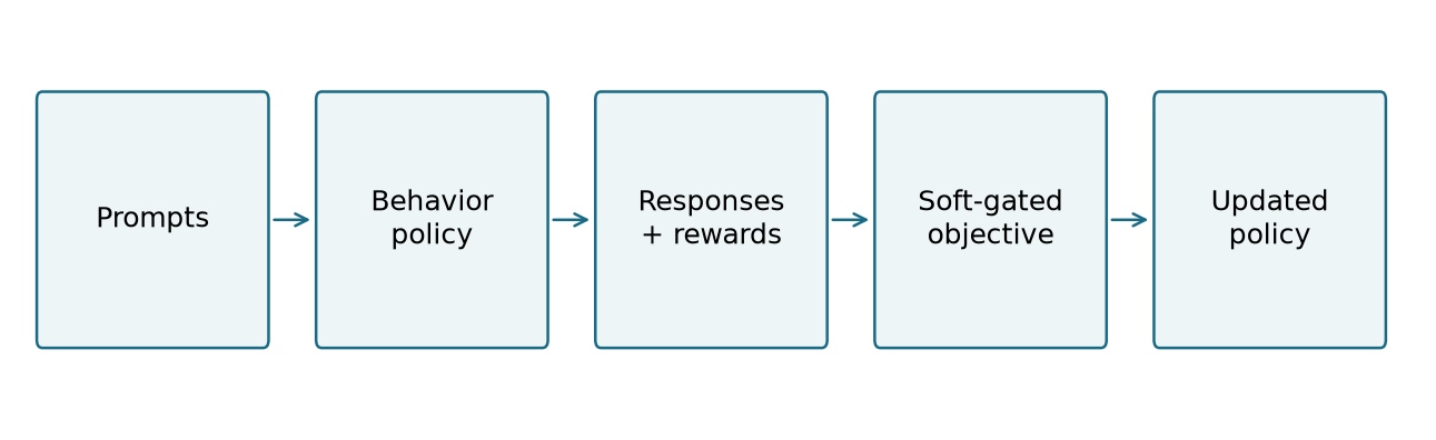
I read SAPO as a proposal about how much to trust each sampled token during a policy update. Its most useful question is operational: after generating answers with yesterday’s policy snapshot, which parts of those answers should still influence today’s parameters? This question appears whenever a rollout batch supports several optimization steps, even without a large asynchronous system.

The core construction uses a sigmoid surrogate whose derivative is a smooth weight. That distinction matters. Multiplying a conventional loss by a sigmoid is generally a different algorithm because automatic differentiation also differentiates the multiplier. In this review I derive the intended derivative, inspect sign-dependent clipping, and separate scalar gate similarity from similarity of full parameter gradients.

The paper is nine pages including references. The longer treatment here is an instructional companion: calculations, counterexamples, implementation reasoning, and suggested experiments are my analysis. The three cropped training figures retain the paper’s measurements; the other six figures are original explanatory diagrams or deterministic calculations. No model training was run for this review. Exact-looking coordinates are not extracted from plotted curves.

A reader familiar with policy gradients can start at Section 5. A reader implementing the objective should read Sections 3, 6, and 10 together. Sections 12 and 13 distinguish the paper’s displayed evidence from what would establish a reliable engineering improvement. The conclusion is deliberately conditional: a smoother local update is useful, but it is not a guarantee of a globally safe training trajectory.

2. Prerequisites: an LLM as a stochastic policy

An autoregressive model gives a probability to each next token. The state at position $t$ is the prompt followed by the already sampled prefix. If the response is $y=(y_1,\ldots,y_T)$, the chain rule gives

$$\pi_\theta(y\mid q)=\prod_{t=1}^{T}\pi_\theta(y_t\mid q,y_{<t}).$$

Taking a logarithm turns a product into a sum:

$$\log\pi_\theta(y\mid q)=\sum_{t=1}^{T}\log\pi_\theta(y_t\mid q,y_{<t}).$$

The score vector $\nabla_\theta\log\pi_\theta(y_t\mid q,y_{<t})$ tells us which parameter changes locally increase the log probability of that sampled token. It is a vector with one component per parameter, not a scalar confidence score. Its magnitude and direction may differ dramatically across tokens.

For a reward $R(y)$ that is fixed with respect to the differentiable policy computation, the likelihood-ratio identity follows by writing $\nabla p=p\nabla\log p$ inside the expectation:

$$\nabla_\theta\mathbb{E}_{y\sim\pi_\theta}[R(y)] =\sum_y R(y)\nabla_\theta\pi_\theta(y) =\mathbb{E}_{y\sim\pi_\theta}[R(y)\nabla_\theta\log\pi_\theta(y)].$$

The identity assumes that the usual interchange of summation and differentiation is valid. If a reward depends differentiably on the policy parameters, its own derivative adds another term. In the sampling-based language-model setting, rewards are normally treated as fixed labels for an update.

Subtracting a baseline that depends only on the prompt does not change the ideal on-policy expectation: the score has mean zero because probabilities sum to one. A baseline reduces variance. A baseline estimated from the same finite response group, however, changes the finite-sample estimator, so practical group-normalized objectives should not automatically inherit every unbiasedness statement about an ideal baseline.

3. Group advantages, masks, and normalization

For one prompt, collect $G$ rewards. Write their population mean and standard deviation as $\bar R$ and $s_R$. A practical fixed advantage is

$$\widehat A_i=\frac{R_i-\bar R}{s_R+\delta},\qquad \bar R=\frac{1}{G}\sum_iR_i,\qquad s_R^2=\frac{1}{G}\sum_i(R_i-\bar R)^2.$$

The small $\delta>0$ is an implementation safeguard, not a claim that the paper specifies this exact constant. If rewards are $(0,1,1,0)$, then $\bar R=0.5$ and $s_R=0.5$; ignoring $\delta$, the advantages are $(-1,1,1,-1)$. All tokens in one response share its advantage. Thus a positive response does not mean every intermediate token was individually useful. Credit assignment remains coarse.

If every reward is the same, the centered rewards are zero. A denominator safeguard should yield zero learning signal, not NaNs. A group containing one rare success can give that success a relatively large normalized advantage. Reward scaling and group composition therefore interact with the gate; the gate does not repair a poor reward definition.

For variable response lengths, SAPO’s displayed objective averages over tokens within each response and then over responses. With mask $m_{i,t}$ and valid length $L_i=\sum_t m_{i,t}$, implement this as

$$J=\frac{1}{G}\sum_{i=1}^{G}\frac{\sum_t m_{i,t}\ell_{i,t}}{L_i}.$$

This differs from pooling every valid token into one large average. Suppose one response has 10 tokens and another has 100. Per-response averaging gives each answer half the total weight; token pooling gives the longer answer roughly ten times as much weight. Neither convention is automatically right for every application. Matching the convention is necessary before comparing algorithms.

Algorithm 1: prepare a response group.

1. Freeze the behavior snapshot and sample $G$ complete responses for each prompt.
2. Store sampled token IDs, valid response masks, and behavior log probabilities.
3. Evaluate rewards using the declared verifier, including truncation and invalid-answer rules.
4. Compute fixed group means, deviations, and normalized advantages.
5. Exclude empty responses explicitly; retain zero-advantage responses without dividing by zero.
6. Keep prompts and padding out of the response loss, and record all normalization choices.

The alternative is a learned value function, which can give richer credit assignment but adds training cost and another approximation. A group estimator is simple and critic-free; it can waste a batch when all sampled rewards coincide. These tradeoffs precede the choice between clipping and a smooth gate.

4. Off-policy ratios and the exact meaning of clipping

Let $b_t$ denote the behavior probability at the sampled prefix and $p_t$ the current-policy probability at the same prefix. Define

$$r_t=\frac{p_t}{b_t}=\exp(\log p_t-\log b_t).$$

The prefix must be identical in the numerator and denominator. Re-generating a prefix under the new policy computes a different quantity. Stored behavior log probabilities stay fixed across optimization steps; replacing them by a freshly evaluated current policy can accidentally make every ratio one.

If $b_t=0.10$ and $p_t=0.12$, then $r_t=1.2$. This is relative probability change, not a probability: ratios can exceed one. A tiny behavior probability makes ratios sensitive to small absolute changes. Log-space subtraction improves arithmetic, but exponentiation can still overflow when a batch is very stale.

A PPO-style scalar surrogate is

$$L(r,A)=\min\{rA,\operatorname{clip}(r,1-\epsilon,1+\epsilon)A\}.$$

Derive its pieces before describing its behavior. For $A>0$, multiplying preserves order, so the objective is $A\min(r,1+\epsilon)$. For $A<0$, multiplication reverses order, giving $A\max(r,1-\epsilon)$. Away from the boundary, its derivative with respect to $r$ is therefore

$$\frac{\partial L}{\partial r}= \begin{cases} A,&A>0,\ r<1+\epsilon,\\ 0,&A>0,\ r>1+\epsilon,\\ A,&A<0,\ r>1-\epsilon,\\ 0,&A<0,\ r<1-\epsilon. \end{cases}$$

Clipping is directional. A positive-advantage token with $r=0.5$ is still active, and a negative-advantage token with $r=2$ is still active when $\epsilon=0.2$. It is inaccurate to say that every token outside a two-sided band loses its gradient. The favorable movement saturates; the movement that worsens the surrogate retains a corrective gradient.

This distinction is central when evaluating SAPO. Its smooth derivative attenuates deviations on both sides, whereas hard clipping is one-sided after conditioning on the advantage sign. Therefore the experiment changes more than differentiability: it also changes which corrective gradients are suppressed. A clean ablation must separate those mechanisms.

5. Deriving SAPO’s soft surrogate

For a positive temperature parameter $\tau$, let $\sigma(u)=1/(1+e^{-u})$. The SAPO construction is

$$f_\tau(r)=\frac{4}{\tau}\sigma\bigl(\tau(r-1)\bigr),\qquad \tau=\begin{cases}\tau_{\rm pos},&A>0,\\\tau_{\rm neg},&A\leq0.\end{cases}$$

The advantage sign selects a fixed temperature during differentiation. The paper’s controlled configuration uses $\tau_{\rm pos}=1.0$ and $\tau_{\rm neg}=1.05$. In the formula, larger $\tau$ makes the gate narrower; the parameter acts like an inverse smoothing width despite being called a temperature.

Take the derivative in three explicit steps. First set $u=\tau(r-1)$. Second use $\sigma'(u)=\sigma(u)(1-\sigma(u))$. Third cancel the chain-rule factor $\tau$ against $1/\tau$:

$$f'_\tau(r)=\frac{4}{\tau}\sigma(u)(1-\sigma(u))\tau =4\sigma(u)(1-\sigma(u))=:w_\tau(r).$$

Because $r=p/b$ and $b$ is fixed,

$$\nabla_\theta r=\frac{\nabla_\theta p}{b} =\frac{p}{b}\nabla_\theta\log p =r\nabla_\theta\log p.$$

Consequently one token contributes $A\,w_\tau(r)\,r\,\nabla_\theta\log p$. At $r=1$, $\sigma(0)=1/2$ and $w_\tau(1)=1$, so the first-order gradient agrees with the unclipped objective for any positive temperature. The scale factor $4/\tau$ is what makes this local agreement hold.

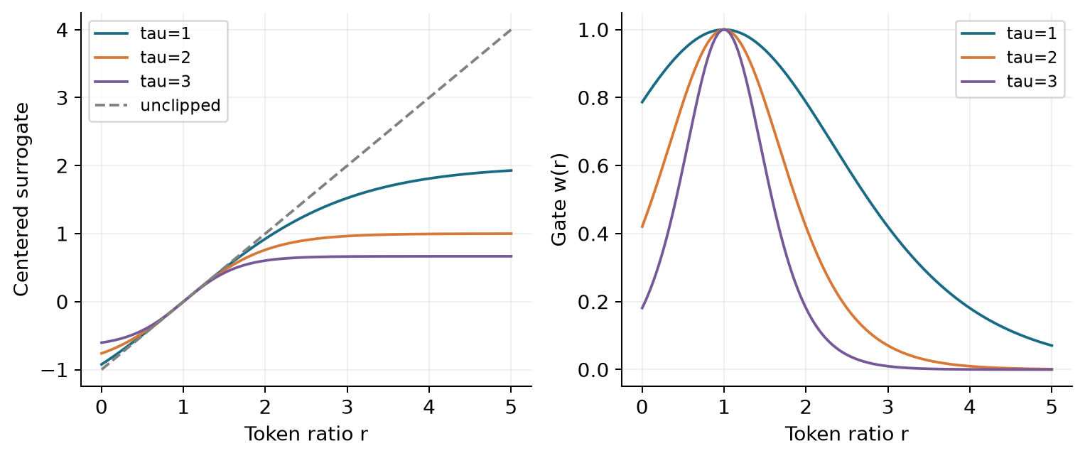
Figure 2 subtracts $f_\tau(1)=2/\tau$ from each curve to align their origins. That subtraction is a constant and does not change gradients. Without it, curves can look different merely because their vertical offsets depend on temperature. Matching objective values is less informative than matching derivatives.

6. Gate weight is not the complete update coefficient

The weight $w$ lies between zero and one, but the multiplier on the score vector is $c(r)=r w(r)$. Bounded $w$ alone is insufficient to explain the update. For example, at $r=2$ and $\tau=1$, $w\approx0.7864$ while $c\approx1.5729$. The token is down-weighted relative to an unclipped importance-weighted update, yet its multiplier exceeds the on-policy value one.

At $r=4$, the corresponding values are approximately $0.1807$ and $0.7228$. At $r=0.5$, they are approximately $0.9400$ and $0.4700$. Small ratios receive a weak coefficient partly because of $r$, not merely because of gate attenuation. These are deterministic evaluations of the displayed formula, not training measurements.

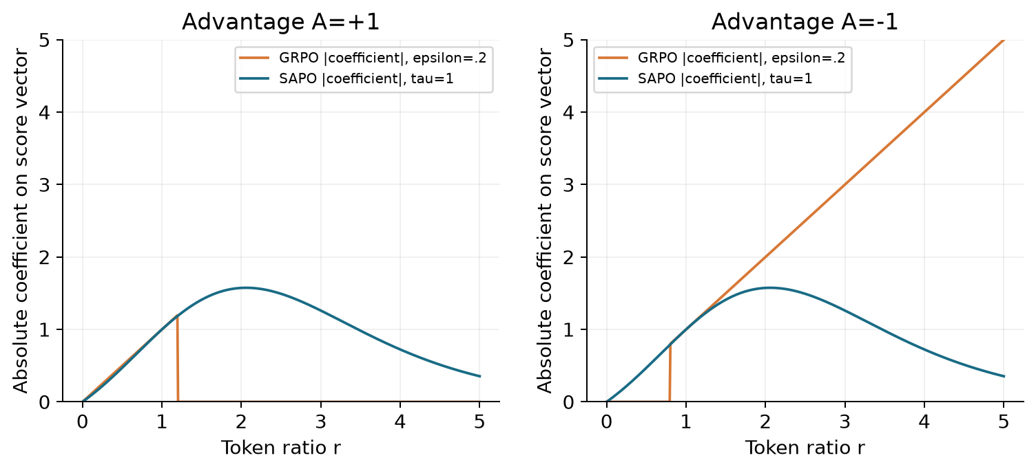
A useful identity makes the shape transparent:

$$w_\tau(r)=\operatorname{sech}^{2}\left(\frac{\tau(r-1)}{2}\right).$$

To derive it, rewrite $\sigma(u)(1-\sigma(u))$ as $1/(e^{u/2}+e^{-u/2})^2$ and use $\cosh(v)=(e^v+e^{-v})/2$. Near $r=1$, put $d=r-1$ and expand:

$$w_\tau(1+d)=1-\frac{\tau^2d^2}{4}+O(d^4).$$

There is no linear attenuation at the center. If $|d|$ is small, changing temperature slightly makes only a second-order local difference. For $\tau=1$ versus $1.05$, the leading difference is $((1.05)^2-1)d^2/4$. At $d=0.1$ this is about $0.000256$. A large long-horizon difference between training runs can therefore reflect rare tails, accumulated feedback, or interacting hyperparameters rather than a large change for a typical near-on-policy token.

For $r\to\infty$, the coefficient behaves like $4r e^{-\tau(r-1)}$ and tends to zero. For $r\to0^+$, the gate approaches a finite positive value while $r w(r)\to0$. These limits do not bound the norm of the full parameter gradient unless score-vector norms and advantages are also controlled. They do not impose a KL constraint either.

The alternative of an explicit KL penalty constrains a different quantity. It can be combined with a gate but adds another coefficient and a reference distribution. Gradient norm clipping also acts at a different level: it rescales an aggregate vector after token contributions have interacted. Treating these mechanisms as interchangeable hides important failure cases.

7. Why positive and negative updates differ

For logits $z_v$ and sampled token $a$, write $p_v=e^{z_v}/\sum_u e^{z_u}$. Differentiating $\log p_a=z_a-\log\sum_u e^{z_u}$ gives

$$\frac{\partial\log p_a}{\partial z_v}=\mathbf{1}[v=a]-p_v.$$

Multiplication by advantage $A$ changes the direction. A positive advantage raises the sampled logit and lowers the alternatives under gradient ascent. A negative advantage reverses every sign. With probabilities $(0.6,0.3,0.1)$ and the first token sampled, the positive gradient is $(0.4,-0.3,-0.1)$; the negative gradient is $(-0.4,0.3,0.1)$.

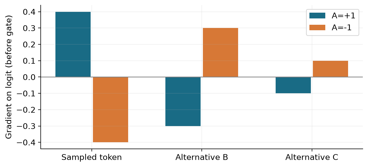
The vocabulary argument needs care. Summing the unsampled magnitudes gives $\sum_{v\ne a}p_v=1-p_a$, regardless of how many vocabulary entries exist. A large vocabulary does not by itself prove a larger total logit-gradient magnitude. The concern is where that pressure goes, how it couples through shared parameters, and how repeated updates affect useful alternatives.

My interpretation is that sign asymmetry is an empirical design hypothesis supported by an ablation, rather than a universal theorem that negative advantages are harmful. Negative updates can eliminate wrong answers, discourage repetitive text, and support exploration. Suppressing them too strongly can preserve undesirable behaviors. A useful test must measure both stability and the ability to unlearn errors.

8. From token ratios to a sequence statistic

For a response of length $T$, let $z_t=\log r_t$. The length-normalized sequence ratio is

$$s=\left(\prod_{t=1}^{T}r_t\right)^{1/T} =\exp\left(\frac{1}{T}\sum_t z_t\right),\qquad \mu=\log s.$$

The geometric mean reduces sensitivity to a single multiplicative outlier compared with the raw sequence product. It can also hide compensating changes: ratios $(2,0.5)$ have geometric mean one, although neither token is on-policy. Thus a sequence statistic is a summary, not a complete measure of distribution mismatch.

SAPO’s relationship to a sequence gate uses two distinct approximations: $r_t$ is close to one, and $z_t$ has small variance within a response. The first gives $r_t-1\approx\log r_t=z_t$. Define

$$g_\tau(z)=\operatorname{sech}^{2}(\tau z/2),\qquad V=\frac{1}{T}\sum_t(z_t-\mu)^2.$$

Taylor-expand each token gate around $\mu$:

$$g_\tau(z_t)=g_\tau(\mu)+g'_\tau(\mu)(z_t-\mu) +\frac12g''_\tau(\xi_t)(z_t-\mu)^2.$$

Averaging cancels the linear term because the centered deviations sum to zero. For $\alpha=\tau/2$, two differentiations give

$$g''_\tau(z)=\alpha^2\bigl(4\operatorname{sech}^2(\alpha z) -6\operatorname{sech}^4(\alpha z)\bigr).$$

Let $u=\operatorname{sech}^2(\alpha z)\in[0,1]$. The polynomial $4u-6u^2$ ranges from $-2$ to $2/3$, so its largest absolute value is two. Therefore $\sup_z|g''_\tau(z)|=\tau^2/2$, yielding

$$\left|\frac1T\sum_tg_\tau(z_t)-g_\tau(\mu)\right| \leq\frac{\tau^2}{4}V.$$

This is a useful, explicit bound on an average of approximate scalar gates. Its strength depends on temperature as well as variance. Saying that variance is small without its scale and $\tau$ is incomplete. The earlier substitution also has error: when $|z|\leq d$, Taylor’s theorem gives $|e^z-1-z|\leq e^d z^2/2$. A gate bound should account for that term separately when ratios are not extremely close to one.

9. Where sequence coherence needs another assumption

The parameter gradient involves a weighted sum of vectors. Define $h_t=\nabla_\theta\log p_t$, $g_t=g_\tau(z_t)$, and $\bar g=T^{-1}\sum_tg_t$. Even after approximating $r_t$ by one, the difference between a token-weighted gradient and a sequence-weighted gradient is

$$\frac1T\sum_t g_t h_t-g_\tau(\mu)\bar h =\frac1T\sum_t(g_t-\bar g)h_t +(\bar g-g_\tau(\mu))\bar h, \qquad \bar h=\frac1T\sum_t h_t.$$

The scalar Taylor bound controls only the second term. The first is a covariance-like term between token weights and gradient directions. An additional bound on score-vector magnitudes and their variation is needed to control it.

By Cauchy-Schwarz, a valid conservative bound for the first term is

$$\left\|\frac1T\sum_t(g_t-\bar g)h_t\right\| \leq \sqrt{\frac1T\sum_t(g_t-\bar g)^2} \sqrt{\frac1T\sum_t\|h_t\|^2}.$$

This makes the missing ingredient visible. A tiny average gate error can coexist with meaningful error in the gradient direction, particularly when token gradients cancel. Relative error becomes unstable near a zero aggregate gradient. It is better to report absolute vector error and cosine similarity with a defined low-norm convention.

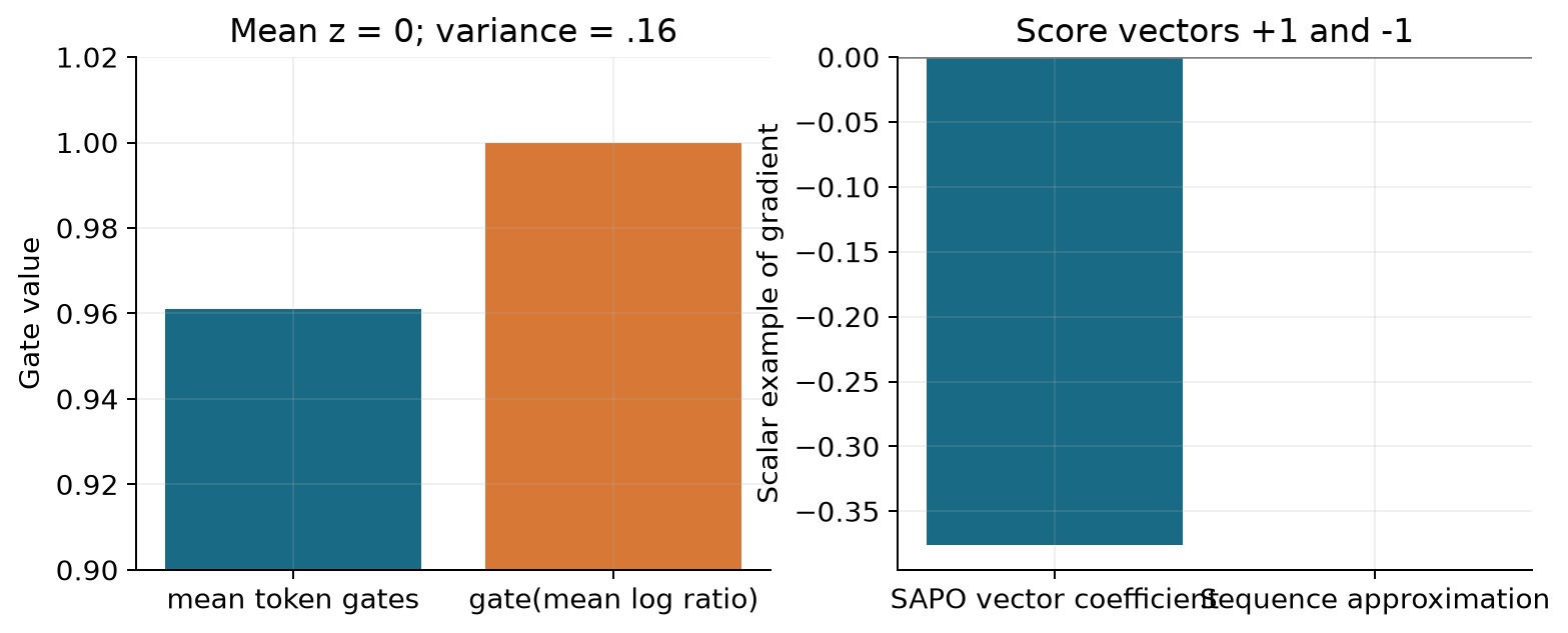
In Figure 5, $z=(-0.4,0.4)$, $\tau=1$, and illustrative score components are $(1,-1)$. The average log ratio is zero. The gap between mean approximate gates and their sequence gate is about $0.0390$, below the $0.04$ variance bound. Nevertheless, the exact SAPO coefficient averaged against those score components is about $-0.3763$, while the sequence approximation is zero. These values are a diagnostic construction, not evidence about the frequency of such a pattern in trained models.

The example uses moderate rather than infinitesimal deviations, so it does not refute a carefully qualified local approximation. It shows why a scalar histogram cannot by itself establish the desired vector statement. A stronger empirical evaluation would measure gradient-vector agreement across actual minibatches, separate dense from MoE models, and stratify by ratio tails and response length.

10. A loss implementation that preserves the intended derivative

A direct implementation differentiates $f_\tau(r)A$ through $r$. A numerically convenient equivalent subtracts the constant at $r=1$:

$$\widetilde f_\tau(r)=\frac4\tau\left[\sigma(\tau(r-1))-\frac12\right].$$

The centered form yields a zero scalar objective at the on-policy point while retaining a nonzero derivative. Therefore zero loss does not imply zero learning. Advantages, behavior probabilities, and chosen temperatures must remain fixed with respect to the current-policy gradient.

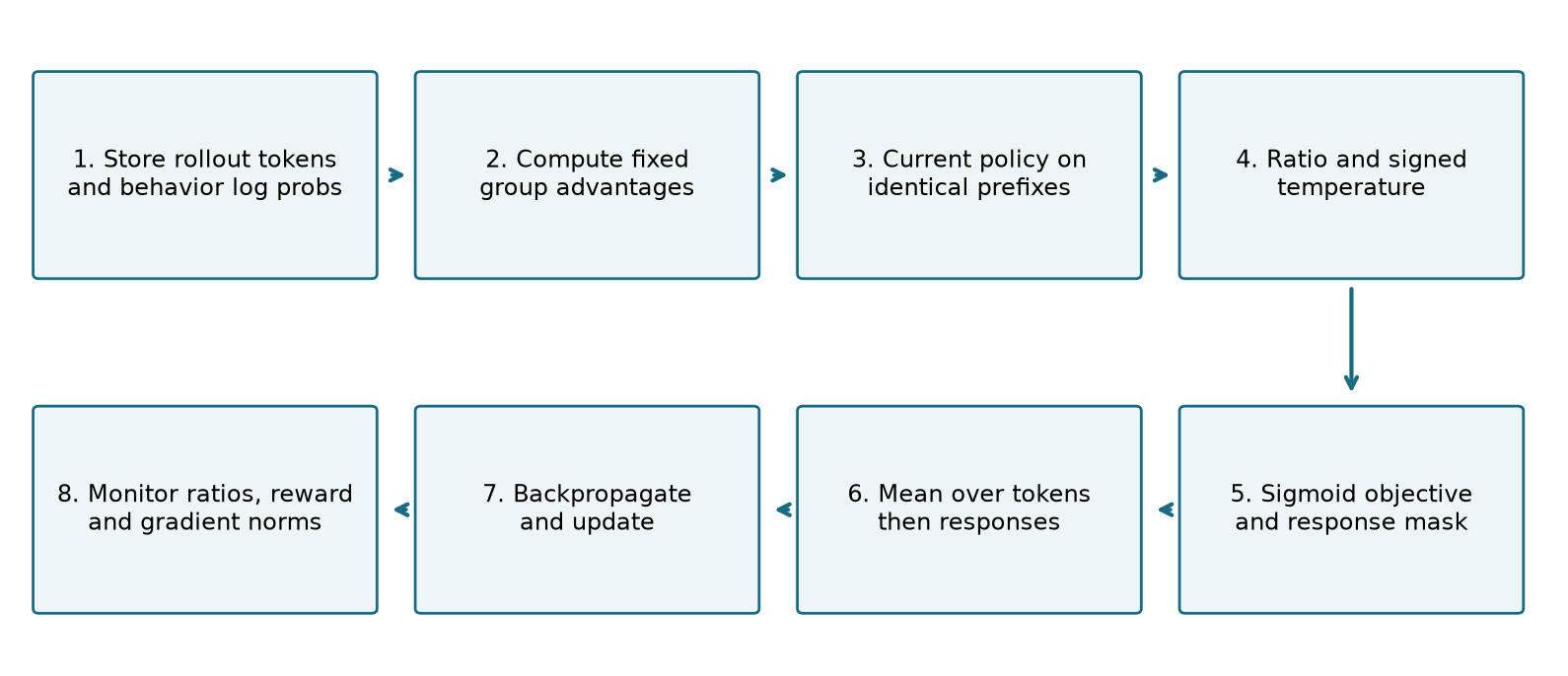
Algorithm 2: one SAPO optimization step.

1. Read a rollout minibatch with frozen behavior log probabilities and advantages.
2. Evaluate current log probabilities by teacher forcing on the stored responses.
3. Subtract behavior log probabilities to obtain $z_t$ and calculate $r_t=e^{z_t}$.
4. Choose $\tau_{\rm pos}$ or $\tau_{\rm neg}$ from the fixed advantage sign.
5. Calculate the centered sigmoid surrogate and multiply by the fixed advantage.
6. Apply the response mask, average by valid response length, then average over the group or batch as declared.
7. Negate the objective when using a minimization optimizer; backpropagate once.
8. Apply the declared optimizer and any separately specified gradient clipping, then record diagnostics.

An alternative implementation treats $Awr$ as a detached weight on $\log p$. It gives the same first-order gradient at the current parameter value if the entire multiplier is detached, but it does not define the same higher-order derivative or scalar objective. Those differences matter for meta-gradients and Hessian-based analysis.

A tempting incorrect expression is $A\,w(r)\,r$ with no stop-gradient. Its derivative contains $A(w(r)+r w'(r))\nabla r$, whereas the desired derivative is $Aw(r)\nabla r$. A second mistake is differentiating through a behavior model that shares current parameters. A third is averaging across padding or prompt tokens. These mistakes can produce smooth-looking training curves while implementing another objective.

Algorithm 3: minimal numerical audit.

1. Use a scalar current log probability and several fixed behavior log probabilities to generate ratios below, at, and above one.
2. Approximate the loss derivative by symmetric finite differences in the current log probability.
3. Compare it with $-A r w(r)$ for a minimization loss, for both signs of $A$ and both temperatures.
4. Check that the derivative at $r=1$ is $-A$ and that zero advantage gives zero gradient.
5. Test equal-reward groups, empty masks, and unequal response lengths separately.
6. Include extreme log ratios to detect numerical failure before attempting a long training run.

For enormous positive log ratios, compute the effective coefficient in log space if using a detached gradient-weight formulation. Since

$$\log w(u)=\log4-\operatorname{softplus}(u)-\operatorname{softplus}(-u), \qquad u=\tau(r-1),$$

one can reason about underflow and overflow explicitly. This identity follows by expanding the two logistic denominators. It is not a complete production implementation: $r=e^z$ itself can overflow, and hard clamping silently changes the objective. A robust system should detect extreme staleness, record it, and apply a declared batch rejection or stabilization policy rather than hiding it inside an undocumented clamp.

11. Design choices and their boundaries

Choice	Why it is useful	Alternative	Boundary to inspect
Token-level gates	Preserve locally useful parts of heterogeneous responses	One sequence-level multiplier	Per-token control does not solve credit assignment
Smooth sigmoid surrogate	Gives continuous derivatives near a clipping threshold	Hard clipping or another smooth kernel	Both tails are attenuated, changing corrective behavior
Separate temperatures	Allows different treatment of signed updates	Shared or adaptive temperature	Too much negative suppression may impair unlearning
Group advantages	Avoid a learned critic	Value baseline or process reward	Equal rewards provide no relative signal
Per-response averaging	Balances responses of different lengths	Token pooling	Changes the length distribution’s effective weighting
Reusing rollout data	Amortizes generation cost	Fresh rollouts after every step	Stale prefixes are not corrected by a local token ratio alone

The last row deserves emphasis. A token ratio compares action probabilities at the observed prefix. It does not fully correct the distribution of prefixes generated by the behavior policy. A complete trajectory importance ratio has different variance and weighting properties. SAPO should be understood as a useful training surrogate, not an automatically unbiased estimator of the new policy’s full trajectory return.

12. Reading the experimental evidence

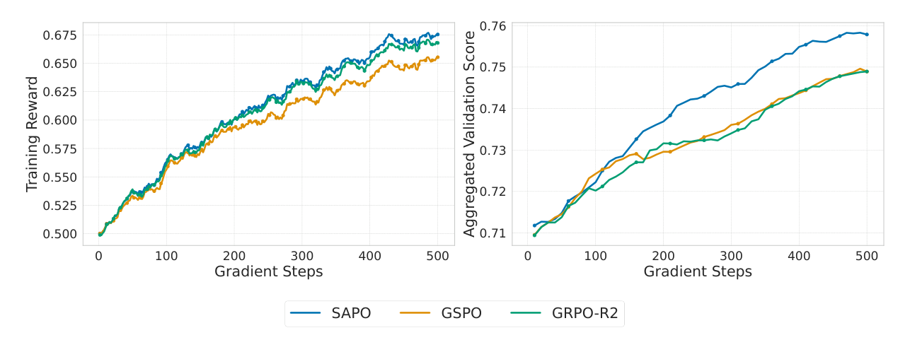
The controlled experiment starts from a cold-start checkpoint based on Qwen3-30B-A3B-Base, uses mathematical queries, and divides each rollout batch into four update minibatches. The reported comparisons include SAPO, GSPO, and GRPO with routing replay. Figure 7 reproduces the original curves; it supports a qualitative comparison over the displayed run, not an exact numerical leaderboard reconstructed from pixels.

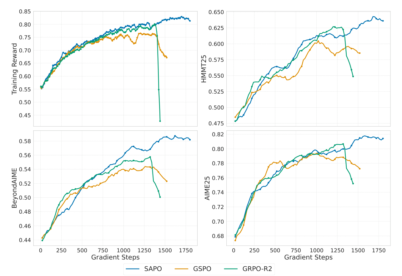
The useful observation is temporal: the curves diverge after an initially shared improvement phase. An endpoint-only comparison can conflate optimization quality with whether a baseline collapsed before the stopping time. I would compare best checkpoint, fixed-step checkpoint, fixed-token checkpoint, and wall-clock budget separately. A method that survives longer can be valuable even if its early sample efficiency is similar.

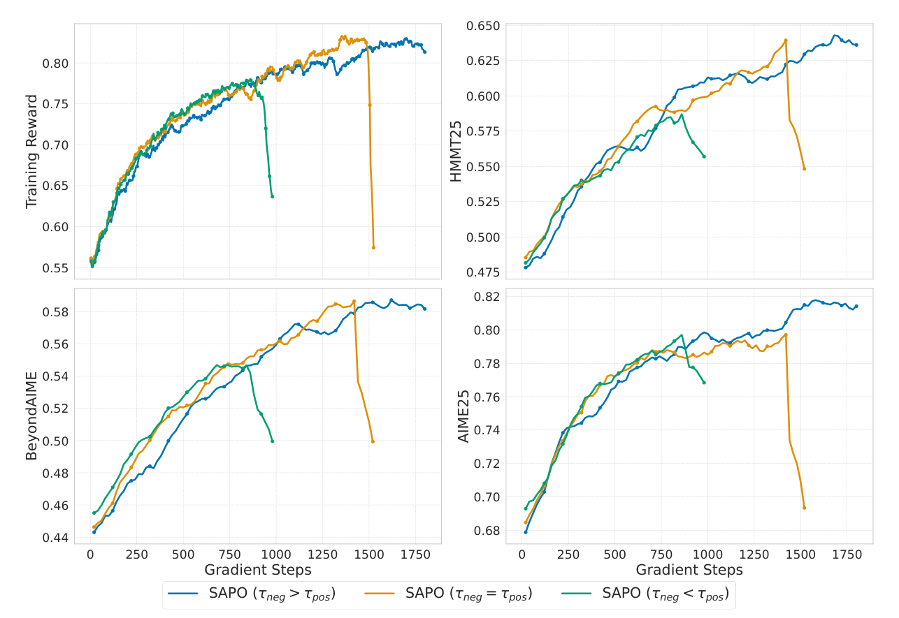
The three displayed temperature choices are informative about this setup. They do not establish a universal optimum. Because near-center weights change only slightly, I would request tail-conditioned gradient statistics and repeated runs to understand the mechanism. The absence of error bars in these figures prevents estimating the variability of collapse time from the visual evidence alone.

The multimodal comparison uses Qwen3-VL-30B-A3B and two update minibatches per rollout batch. The paper reports evaluations involving AIME25, LiveCodeBench v6, ZebraLogic, and MathVision. Different numbers of sampled responses are used to estimate Pass@1 in different evaluations; this is not the same metric as Pass@k. The average of many independent single-sample correctness indicators estimates the chance that one sample succeeds. It does not estimate the chance that at least one of all samples succeeds.

An aggregate score also requires task weights and uncertainty. For task scores $a_j$ and weights $\lambda_j$, an aggregate $\sum_j\lambda_j a_j$ may improve even when one task regresses. I would retain the per-task breakdown, evaluation prompts, decoding parameters, and any benchmark contamination checks. None of these can be recovered reliably from a single aggregate curve.

13. Limitations and reproducibility

The loss is compact; a matching experiment is not. A reproducible comparison needs the initial checkpoint, prompt and reward distributions, optimizer, learning-rate schedule, rollout group size, response length limits, update batch sizes, sampling temperature, routing policy, and evaluation protocol. Referring to another algorithm’s configuration helps locate information but does not substitute for one complete, versioned configuration.

A verifier can also be wrong. Reward hacking, ambiguous answer extraction, and truncation can create misleading advantages. Smoothing a gradient derived from an incorrect reward does not make the reward correct. Dataset quality and solver evaluation remain separate responsibilities.

The displayed experiments do not give a theorem ruling out collapse, a uniform claim over model sizes, or a causal decomposition of every benefit. Their value is to motivate controlled follow-up work. This review did not reproduce model training; the local numerical checks concern the stated objective and explanatory examples only.

14. Independent critical analysis

14.1 A scalar-to-vector step needs stronger justification

The main theoretical concern is the transition from average scalar gates to a full sequence-style gradient. Section 9 isolates the covariance term. An actionable improvement is to state a bound containing score-vector norms and gate-gradient dependence, then measure both terms on training batches. A scalar $D$ versus variance plot alone cannot certify alignment of parameter updates.

14.2 Smoothness is entangled with bidirectional suppression

The hard-clipped baseline and the smooth method differ in the treatment of corrective updates outside the opposite boundary. To identify which mechanism helps, compare four variants under equal tuning budgets: directional hard clipping, directional smooth clipping, bidirectional smooth attenuation, and a different smooth kernel with matched local slope and width. Report both validation quality and the fraction of signed learning signal removed.

14.3 The negative-token explanation is incomplete as a norm argument

The softmax derivative redistributes pressure over alternatives, but total unsampled probability mass is bounded by one. More vocabulary entries do not alone produce a larger logit-gradient norm. A sharper explanation would examine probability concentration, score-vector norms, MoE routing transitions, and reward sign together. Measure whether instability correlates with these quantities after controlling for advantage magnitude and policy lag.

14.4 Fairness requires a budget for retuning baselines

Identical hyperparameters do not guarantee equally strong baselines. A new optimizer may simply tolerate settings that are poor for another. Report both a shared-configuration comparison and an equal-search-budget comparison. Keep rollout tokens, optimizer steps, verifier calls, and wall-clock cost explicit. Include several seeds and a prespecified collapse criterion rather than choosing a favorable endpoint after observing the trajectories.

14.5 Stability should include the cost of conservatism

A stable run that learns too slowly is not necessarily a better run. Track reward gains per generated token, time to reach a validation threshold, response length, entropy, and failure to suppress known bad behaviors. A stronger temperature can remove exactly the negative feedback required to correct systematic errors. Targeted unlearning probes would reveal this tradeoff more clearly than aggregate reward alone.

15. A concrete follow-up experiment

I would start with a small model and a fixed, auditable mathematical task set. Freeze the data split before examining curves. Use one loss implementation and vary only the gating function, with routing behavior and normalization explicitly held constant.

Algorithm 4: compare optimization behavior without hiding costs.

1. Reserve development prompts for tuning and untouched evaluation prompts for reporting.
2. Allocate the same number of configurations and random seeds to every method.
3. Record rollout tokens, update tokens, optimizer steps, verifier calls, and elapsed time.
4. Log advantage sign, ratio quantiles, $rw(r)$ quantiles, zero-advantage groups, response lengths, and gradient norms.
5. Sample batches for token-versus-sequence gradient cosine similarity and absolute error.
6. Report taskwise Pass@1 with uncertainty, collapse timing, and best versus final checkpoint results.
7. Repeat with increased rollout lag and longer outputs to test the intended failure boundary.

This proposal is a reproducibility plan, not a completed experiment or a claim about likely numerical gains. Its purpose is to distinguish smoother optimization, stronger conservatism, and better use of heterogeneous samples.

16. Conclusion

SAPO offers a small and interpretable change to a group-based policy objective. Its derivative can be derived exactly, audited cheaply, and understood at both token and sequence scales. I find the implementation idea compelling, while treating broad stability claims and sequence equivalence as questions that need stronger qualification. The most useful next step is a controlled comparison that measures the full update vector and the cost of discarded learning signal, alongside downstream scores.

References and evidence notes

• Gao et al. Soft Adaptive Policy Optimization, v2, 2025. Primary paper; all reproduced training curves are cropped from its Figures 4–6. The note adds original derivations and criticism rather than reproducing its text.
• Shao et al. DeepSeekMath, 2024. Background for the group-relative policy objective; the comparison here uses the precise objective written in SAPO.
• Zheng et al. Group Sequence Policy Optimization, 2025. Background for geometric-mean sequence ratios.
• Qwen SAPO research announcement. Author-team account; distinguish its qualitative interpretation from independent validation.
• ModelScope ms-swift SAPO documentation. An independently maintained implementation reference; not evidence that this review ran that code or reproduced the paper’s training setup.

Source and discussion checks were performed on 2026-09-15. The paper is an existing work from 2025, selected to fill a gap in the current reading collection, not presented as a newly released paper.