When Sparse Capacity Meets Repeated Data: A Technical Review of MoE Overfitting

Review date: 2026-09-12
Author: Zhongzhu Zhou
Paper reviewed: Data Scarcity and Model Sparsity: Mixtures-of-Experts Overfit More to Repeated Data
Paper authors: Atindra Jha, Margaret Li, Jure Leskovec, Percy Liang, Luke Zettlemoyer
arXiv: 2609.11917v1
Venue / status: Preprint, September 2026

1. Why this paper matters

Modern scaling recipes quietly assume that a token seen twice is almost as useful as two different tokens. That assumption becomes dangerous when high-quality text is scarce. Training then has two budgets: total processed tokens, which determine compute, and unique tokens, which determine how many independent observations constrain the model.

Mixture-of-Experts (MoE) models add another split. A token activates only a small subset of the parameters, so active parameters determine most arithmetic cost while total parameters determine representational capacity. The paper asks what happens when both decouplings occur together: total versus unique tokens, and active versus total parameters.

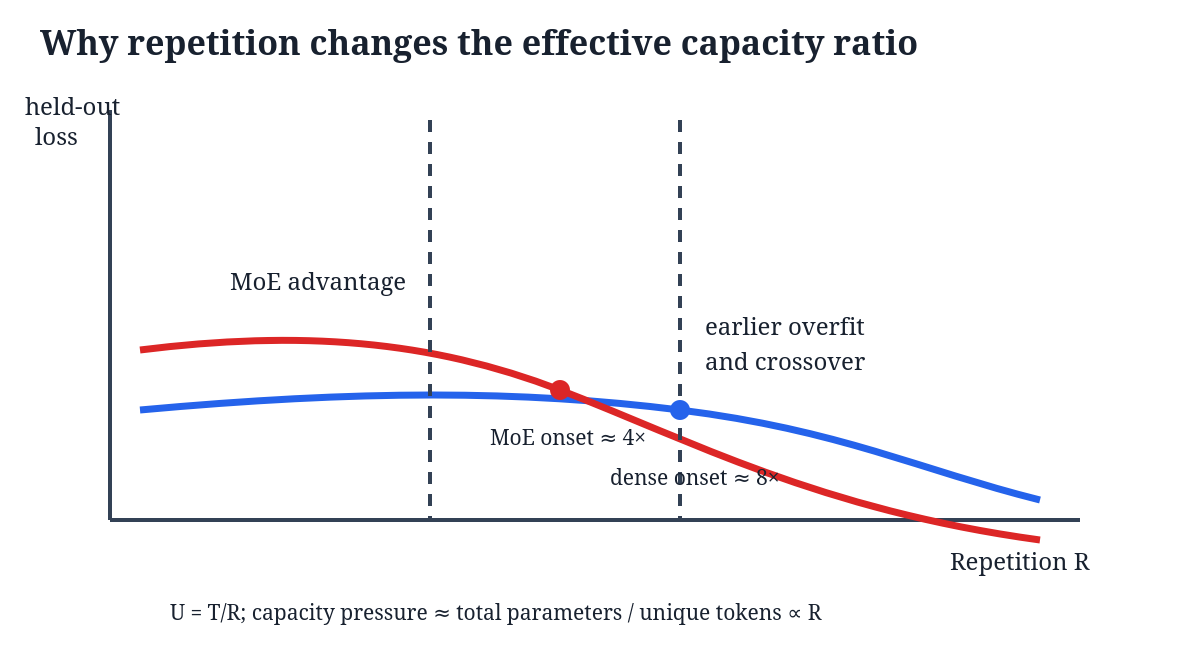
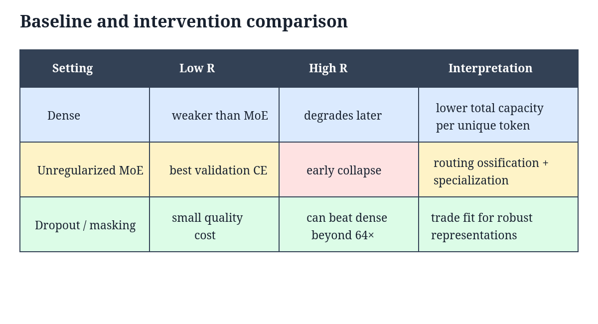
Its central result is memorable: under all-unique data, sparse models are better at equal active compute; under heavy repetition, they overfit earlier and can become much worse than dense models. At the 80M-active scale, degradation is visible around four repetitions for MoE and around eight for dense models. Near 32 repetitions, the ordering can reverse. Strong masking-based regularization can delay the collapse, but cannot recreate information that is absent from the unique corpus.

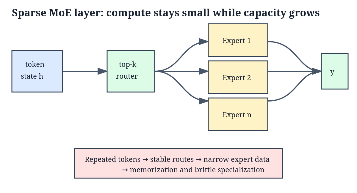
The figure summarizes my reading of the causal story. The router repeatedly sends familiar tokens to nearly the same experts. Those experts see a narrower, increasingly stationary sample and can memorize it. This is plausible, but the paper mainly establishes correlations and interventions around that story rather than a complete causal proof.

2. Prerequisites

2.1 Dense Transformer feed-forward blocks

A Transformer layer contains attention and a position-wise feed-forward network (FFN). For token state $h$, a simplified SwiGLU FFN is

$$\operatorname{FFN}(h)=W_2\left(\operatorname{SiLU}(W_g h)\odot W_1 h\right).$$

Every token uses every FFN weight. Therefore the model’s total parameter count and per-token active parameter count are nearly the same. More parameters normally mean both more capacity and more floating-point work.

Cross-entropy measures next-token prediction quality. If the correct next token is $x_t$, the per-token loss is

$$\ell_t=-\log p_\theta(x_t\mid x_{<t}).$$

Averaging over $N$ held-out tokens gives

$$L_{\mathrm{val}}(\theta)=\frac{1}{N}\sum_{t=1}^{N}\ell_t.$$

The derivation is direct: maximum likelihood maximizes $\prod_t p_\theta(x_t\mid x_{<t})$; taking a negative logarithm converts the product into a sum. Lower held-out cross-entropy means the model assigns more probability to unseen text. Falling training loss together with rising validation loss is the signature used here for memorization.

2.2 Sparse Mixture-of-Experts

An MoE replaces the dense FFN with $n$ expert FFNs $E_1,\ldots,E_n$. A router computes logits

$$s(h)=W_r h.$$

For the selected set $S(h)=\operatorname{TopK}(s(h),k)$, normalized gates are

$$g_i(h)=\frac{\exp s_i(h)}{\sum_{j\in S(h)}\exp s_j(h)},\qquad i\in S(h).$$

The output is then

$$y(h)=\sum_{i\in S(h)}g_i(h)E_i(h).$$

Only $k$ experts run, although all $n$ experts are stored. If each expert has fraction $g$ of a dense FFN’s width and $k=1/g$, active expert capacity is approximately dense-equivalent. Total expert capacity, however, scales like $ng$. A useful sparsity factor is

$$S=\frac{N_{\mathrm{total}}}{N_{\mathrm{active}}}.$$

This is why an 80M-active MoE can contain hundreds of millions of total parameters without paying that full cost per token.

2.3 Repetition creates two token budgets

Let $T$ be total processed training tokens and $U$ the number of unique tokens. The repetition rate is

$$R=\frac{T}{U}.$$

Holding compute fixed means holding $T$ fixed. Increasing $R$ therefore forces

$$U=\frac{T}{R}.$$

Double $R$, and each model sees only half as many unique constraints. A dense model’s rough capacity-per-unique-token ratio is $N_{\mathrm{dense}}/U$. For an MoE it is more revealing to use total parameters:

$$\frac{N_{\mathrm{total}}}{U} =\frac{N_{\mathrm{total}}R}{T}.$$

Thus repetition linearly increases total capacity per unique token. This does not prove overfitting, but it explains why total rather than active parameters can govern the onset.

3. Experimental design

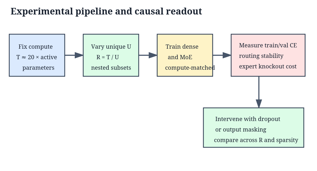
The authors train compute-matched dense and sparse decoder-only Transformers at 80M, 200M, and 1B active parameters. The largest MoE has 8.5B total parameters. Their default token budget follows a Chinchilla-style rule,

$$T\approx 20N_a,$$

where $N_a$ is active parameters. They sweep $R$ from 1 through 1024 in core experiments, changing $U=T/R$ while keeping $T$ fixed.

MoE configurations vary expert count $n\in\{8,16,32,64,128\}$ and expert granularity $g\in\{1/2,1/4,1/8,1/16,1/32\}$. They set $k=1/g$ to approximately match active parameters. This separates two questions: does merely storing more experts matter, and does making each expert larger matter?

Training data comes from the OLMoE mixture and four isolated domains: DCLM web text, StarCoder code, peS2o scientific text, and Wikipedia. Validation uses matched held-out domains plus Paloma-style language modeling corpora and downstream BoolQ, HellaSwag, and MMLU measurements.

3.1 Algorithm 1 — construct nested repeated datasets

Nested subsets are important. If each value of $R$ used a separately sampled corpus, changes in quality could masquerade as repetition effects.

Algorithm 1: Nested unique-token sweep
Inputs: shuffled corpus D, active parameters Na, repetition rates R_set
1. Set total token budget T <- 20 * Na.
2. Draw one fixed random permutation pi(D).
3. For each repetition rate R in R_set:
4.     Compute unique budget U <- floor(T / R).
5.     Take D_U <- first U tokens of pi(D).
6.     Repeat D_U for R epochs, reshuffling sequence order each epoch.
7.     Ensure exactly T tokens are processed.
8.     Train the candidate architecture with the shared schedule.
9.     Evaluate training CE, held-out CE, and downstream metrics.
10. Return metrics indexed by architecture, scale, and R.

Why it works. For $U_1\le U_2$, the construction guarantees $D_{U_1}\subseteq D_{U_2}$. High-repetition runs contain less information, not an unrelated sample.

Obvious alternative. Independently sample a fresh $U$-token set for every run. That is easier in distributed data loaders but confounds repetition with sample difficulty.

Boundary. Nesting makes comparisons internally clean, yet one permutation can still be atypical. The paper repeats selected 80M settings over five initialization seeds, not many independent data permutations. Seed variance is small for validation loss but larger for some downstream losses.

3.2 Fairness of the compute match

Equal active parameters is a reasonable FLOP-oriented control because only selected experts execute. It is not a full system-cost match. More experts increase memory footprint, all-to-all traffic, routing overhead, and optimizer state. Therefore the claim is not that MoE is equally cheap in every resource. It is that, at approximately equal token-level neural compute, sparse capacity responds differently to repeated information.

The distinction matters for interpreting a crossover. Once the MoE has worse validation loss than dense at $R=32$, it is also likely consuming more memory and communication. In that regime its practical advantage is doubly weakened.

4. Main empirical result: sparsity amplifies repetition damage

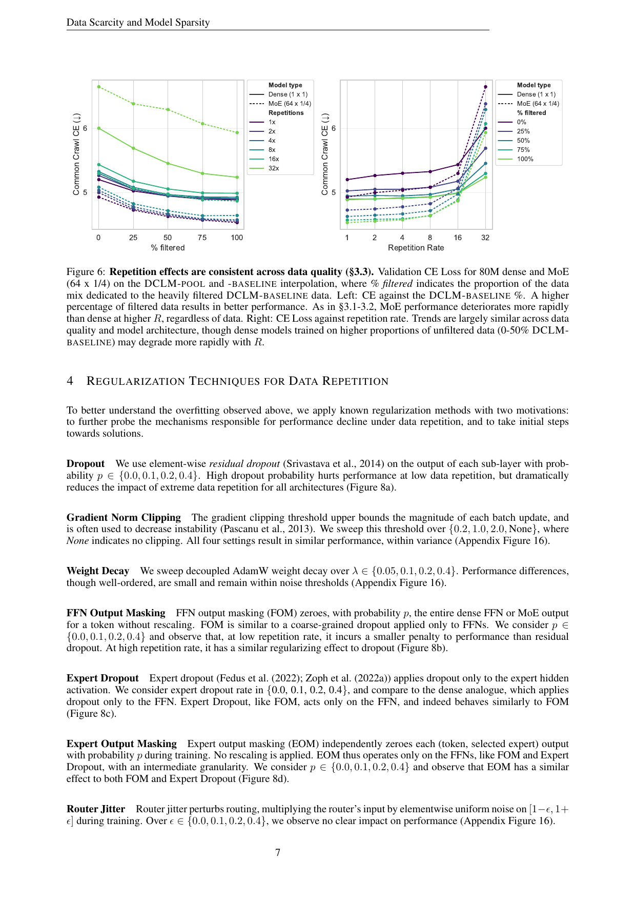
The first plot is the paper’s most important evidence. At low $R$, MoEs have lower validation loss than dense controls. Increasing $R$ initially leaves dense models almost unchanged, while sparse models bend upward sooner. Around $R=32$, dense can overtake MoE.

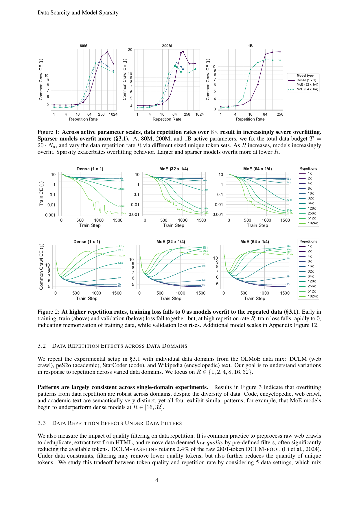
The train/validation split rules out simple under-training. At high repetition, training cross-entropy approaches zero while held-out loss rises. Let

$$G(R)=L_{\mathrm{val}}(R)-L_{\mathrm{train}}(R)$$

be a generalization gap. Compare two repetition rates $R_2>R_1$:

$$\Delta G= \left[L_{\mathrm{val}}(R_2)-L_{\mathrm{val}}(R_1)\right] -\left[L_{\mathrm{train}}(R_2)-L_{\mathrm{train}}(R_1)\right].$$

At severe repetition, the first bracket is positive while the second is negative. Therefore $\Delta G$ is strongly positive: optimization fits the repeated stream better, but the learned predictor generalizes worse.

An unusual non-monotonic region appears at extremely high repetition: loss can improve after an intermediate worst point, then rise again at still larger $R$. This warns against fitting a simple monotone law from a narrow sweep. A plausible explanation is a change between partial memorization and near-complete fitting, but the study does not identify a definitive mechanism.

4.1 Total parameters, not active parameters

Two architecture sweeps support the total-capacity explanation:

• Holding expert granularity fixed while adding experts increases total parameters and worsens sensitivity.
• Holding expert count fixed while enlarging experts also increases total parameters and worsens sensitivity.
• Curves with similar total parameter counts look more alike even when their active counts or architectural decomposition differ.

A useful hypothesis is that damage depends on

$$ho=\frac{U}{N_{\mathrm{total}}} =\frac{T}{RN_{\mathrm{total}}},$$

the unique-token-to-total-parameter ratio. Increasing either $R$ or $N_{\mathrm{total}}$ lowers $ho$. This equation is an interpretive lens, not a fitted theorem \in the paper; no universal threshold $ho^star$ is established.

4.2 Domain robustness and filtering

The phenomenon repeats on web, code, scientific, and encyclopedic text. MoEs generally begin losing their edge between $R=16$ and $R=32$. This breadth is valuable because a result restricted to one crawl might only reflect duplicate boilerplate or noisy pages.

Heavy quality filtering improves absolute loss, but does not eliminate the sparse-model pattern. In one direct trade-off, one pass over a much larger unfiltered pool beats 32 passes over the heavily filtered subset. The correct operational lesson is not “never filter.” It is to jointly optimize quality and unique quantity. A filter that removes 97.6% of tokens can force enough repetition to erase its quality benefit.

4.3 Mixed domains

When repeated StarCoder or peS2o data is mixed with unrepeated DCLM, degradation mostly stays within the repeated domain. Unrepeated web text can regularize repeated scientific text, especially when it occupies a substantial share. The effect is weaker for code, perhaps because web and scientific prose share more representations than web and code.

Why this design works. Domain-specific $R_i$ resembles real pretraining mixtures.

Alternative. Use one global repetition rate. That is cleaner but hides which domain causes the failure.

Boundary. Only a few two-domain mixtures are tested. Semantic similarity is proposed as an explanation, yet not measured with a controlled similarity variable.

5. Regularization: what helps and what does not

The paper sweeps residual dropout, gradient clipping, weight decay, router jitter, expert dropout, FFN output masking, and expert output masking. The strongest pattern is that stochastic removal of activations or whole outputs helps at high $R$. Gradient clipping and the tested weight-decay range change little; router jitter also fails to address the core problem.

For inverted element-wise dropout with mask $m_jsimoperatorname{Bernoulli}(1-p)$,

$$\widetilde z_j=\frac{m_j}{1-p}z_j.$$

Its expectation is preserved:

$$\mathbb E[\widetilde z_j] =\frac{\mathbb E[m_j]}{1-p}z_j =\frac{1-p}{1-p}z_j =z_j.$$

Yet any one training step sees a random subnetwork. Repeated examples cannot rely on exactly the same co-adapted feature path every epoch.

FFN output masking is coarser. For a token-level Bernoulli variable $b$,

$$\widetilde y=b,y,\qquad bsimoperatorname{Bernoulli}(1-p),$$

without rescaling in the paper’s implementation. This deliberately biases the expected branch magnitude to $(1-p)y$, but forces the residual stream to remain useful when the FFN branch disappears.

5.1 Algorithm 2 — repetition-aware regularizer selection

Algorithm 2: Select a regularizer under a unique-data constraint
Inputs: candidate probabilities P, repetition regimes R_set, dense control
1. For each regularizer family q:
2.     For each probability p in P:
3.         Train matched models at both low and high repetition.
4.         Record held-out CE L(q,p,R).
5.         Compute low-R cost C_low <- L(q,p,R_low)-L(no_reg,R_low).
6.         Compute high-R gain G_high <- L(no_reg,R_high)-L(q,p,R_high).
7.         Reject settings that improve only training loss.
8.         Retain Pareto settings with small C_low and large G_high.
9. Compare retained MoEs against the dense control at the same active scale.
10. Choose p from the expected production repetition range, not one global default.

Why it works. It makes the central trade-off explicit. Strong dropout hurts the information-rich regime but can dramatically improve the scarce-data regime.

Obvious alternative. Tune only at $R=1$ and reuse that hyperparameter. This selects too little regularization for repeated data.

Boundary. The best $p$ is model-size and schedule dependent. The paper itself notes that dropout requires retuning. A result at 80M or 200M cannot be copied blindly to trillion-parameter training.

5.2 Why clipping and moderate weight decay may fail

Gradient clipping bounds unusually large updates:

$$\widetilde g= g\min\left(1,\frac{c}{\lVert g\rVert_2}\right).$$

Repeated-data memorization need not involve rare gradient explosions. Many small, consistent updates toward the same examples can remain below $c$, so clipping leaves the process intact.

Decoupled weight decay applies approximately

$$\theta_{t+1}=(1-\eta\lambda)\theta_t-\eta\,\widehat g_t.$$

It discourages large weights but does not directly diversify features or routes. The tested $\lambda$ range may simply be too weak; prior dense-model work found benefit from much stronger decay, paid for by worse single-epoch loss. Therefore “weight decay cannot help” would overstate the evidence.

6. Mechanistic probes: routing ossification and specialization

6.1 Routing stability

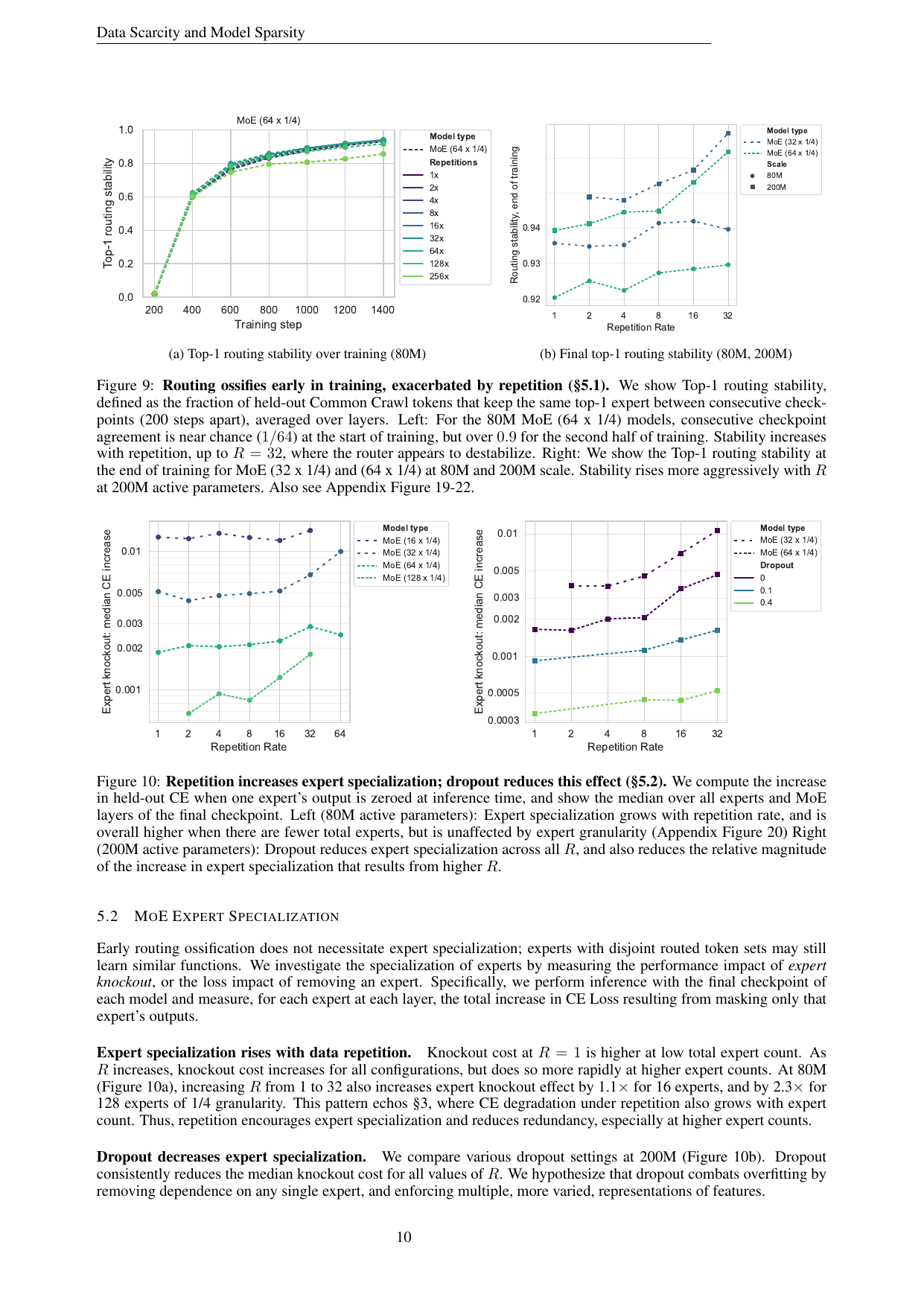
For a fixed held-out batch, let $a_t(x,\ell)$ be the top-1 expert selected for token $x$ at layer $\ell$ at checkpoint $t$. Consecutive-checkpoint stability is

$$S_t= \frac{1}{|\mathcal X|L} \sum_{x\in\mathcal X} \sum_{\ell=1}^{L} \mathbf 1\!\left[a_t(x,\ell)=a_{t-\Delta}(x,\ell)\right].$$

The indicator is one when the route does not change. Averaging makes $S_t$ the empirical probability that a token-layer pair keeps its preferred expert over the checkpoint interval. Stability rises very early—within roughly the first ten percent of training—and repetition raises the final value slightly.

6.2 Algorithm 3 — measure router ossification

Algorithm 3: Consecutive-checkpoint top-1 routing stability
Inputs: checkpoints theta[0..M], fixed validation batch X, MoE layers 1..L
1. Disable all train-time noise and regularizers.
2. For checkpoint t from 0 to M:
3.     Run X through the model.
4.     Save top1[t,x,l] <- argmax_i router_score_i(x,l).
5. For t from 1 to M:
6.     matches <- 0.
7.     For each token x and layer l:
8.         matches += 1[top1[t,x,l] = top1[t-1,x,l]].
9.     stability[t] <- matches / (|X| * L).
10. Return the stability curve and mean of the final intervals.

Why it works. The batch is fixed, so route changes reflect changing router parameters rather than changing input samples.

Alternative. Compare routing distributions using KL divergence. That captures soft-score changes but can report movement even when the executed top-$k$ set is identical.

Boundary. The metric uses top-1 even when multiple experts are active. Stable top-1 does not imply a stable full top-$k$ set or stable gate weights. Checkpoint spacing also changes the numeric value, so only matched intervals are comparable.

6.3 Expert knockout as specialization

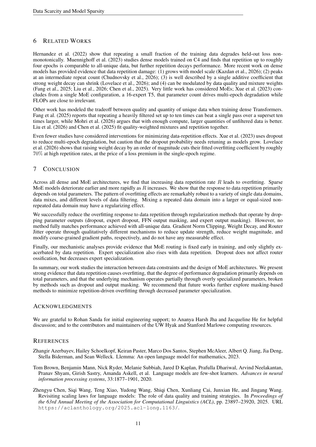
At the final checkpoint, the authors zero one expert’s output while leaving the router and other gates untouched. If baseline held-out loss is $L$ and loss after removing expert $e$ at layer $\ell$ is $L_{-\ell,e}$, define knockout cost

$$K_{\ell,e}=L_{-\ell,e}-L.$$

Large $K_{\ell,e}$ means the rest of the network cannot compensate for that expert. The median cost grows with repetition. At 80M active parameters, moving from $R=1$ to $R=32$ raises the effect by about $1.1\times$ for 16 experts and $2.3\times$ for 128 experts at quarter granularity. Dropout lowers knockout cost.

6.4 Algorithm 4 — expert knockout audit

Algorithm 4: Expert specialization by output knockout
Inputs: final model theta, fixed batch X, all expert locations (l,e)
1. Compute baseline held-out CE L on X.
2. For every MoE layer l:
3.     For every expert e in layer l:
4.         Keep router scores and selected expert sets unchanged.
5.         Replace expert output E_l,e(h) with zero.
6.         Do not renormalize the remaining gates.
7.         Recompute held-out CE L_minus[l,e].
8.         Set K[l,e] <- L_minus[l,e] - L.
9. Summarize K by median and maximum over layers and experts.
10. Compare summaries across repetition, expert count, and dropout.

Why it works. It is an intervention, not merely a correlation between router statistics and loss.

Alternative. Measure cosine similarity between expert weights or outputs. Similarity is cheap, but functionally different experts may have similar weights and vice versa.

Boundary. Because gates are not renormalized, knockout changes both represented function and output scale. A redundancy-aware test could reroute tokens to their next-best expert and separate missing function from missing magnitude.

6.5 Co-activation entropy

For each layer, count how often unordered expert pair ${i,j}$ appears together in a token’s top-$k$ set. Normalize counts into $p_{ij}$. Shannon entropy is

$$H=-\sum_{i<j}p_{ij}\log p_{ij}.$$

With $n$ experts, there are $\binom n2=n(n-1)/2$ unordered pairs. A conventional normalization would divide by $\log\binom n2$. The paper describes normalization using a maximum based on $n(n-1)$; either convention only differs by a constant inside the logarithm, but the exact implementation should be documented for replication. Normalized entropy near one means diverse expert pairings; lower entropy means a narrow co-activation pattern.

Dropout increases co-activation entropy while reducing knockout specialization. Together these observations suggest that stochastic removal discourages a few fixed expert coalitions from becoming indispensable.

6.6 From correlation to a candidate mechanism

The evidence can be organized as a chain:

1. Higher $R$ reduces unique tokens while leaving updates and compute fixed.
2. Router choices stabilize early, repeatedly assigning similar examples to similar experts.
3. Each expert receives a narrower effective dataset than the global corpus.
4. Expert knockout cost grows, indicating less functional redundancy.
5. Validation loss rises earlier for configurations with more total capacity.
6. Dropout or output masking reduces specialization and improves high-$R$ loss.

Steps 2–4 are measured, and step 6 is intervention evidence. But the chain is not fully identified. A hidden factor—such as feature learning in the shared attention blocks—could independently drive stable routing and specialization. A stronger causal study would deliberately reset or randomize routers mid-training while controlling optimizer state, then observe whether specialization and held-out loss recover.

7. Translating the result into a training decision

Suppose a project has compute budget $T$, unique data budget $U$, and candidate dense/MoE architectures. The naive decision uses only active parameters. A repetition-aware decision should estimate

$$R_{\mathrm{eff}}=\frac{T}{U_{\mathrm{eff}}},$$

where $U_{\mathrm{eff}}$ discounts near-duplicates, templated documents, and low-diversity synthetic variants.

A practical workflow is:

1. Deduplicate and cluster the corpus before choosing model sparsity.
2. Report both raw tokens and estimated unique tokens per domain.
3. Compute per-domain $R_i=T_i/U_i$ under proposed mixture weights.
4. Run small proxy models across the same $R_i$ range.
5. Track training CE, held-out CE, router stability, and knockout cost.
6. Tune dropout or FFN masking at both low and high $R$.
7. Prefer dense or less-sparse models when the expected regime lies beyond the MoE crossover.

7.1 A simple break-even model

Let low-repetition MoE gain over dense be

$$A(R)=L_{\mathrm{dense}}(R)-L_{\mathrm{MoE}}(R).$$

MoE is preferable in quality when $A(R)>0$. Define the crossover

$$R^star=\inf{R:A(R)\le 0}.$$

In this paper, $R^star$ is often near 32 for the tested 80M settings, but it varies with scale, architecture, domain, and regularization. Production should estimate its own $R^star$, not copy the number.

If systems cost matters, augment loss with a resource penalty:

$$J=L_{\mathrm{val}}+\alpha C_{\mathrm{compute}}+\eta C_{\mathrm{memory}}+\gamma C_{\mathrm{network}}.$$

Equal active parameters roughly control the first cost, but not the latter two. High repetition can therefore move both the quality term and the infrastructure terms against MoE.

8. Experimental results in numbers

The five-seed appendix makes the crossover concrete at 80M active parameters. On the average language-modeling validation set:

• Dense, $R=1$: $4.81pm0.01$.
• Dense, $R=32$: $5.48pm0.05$.
• MoE (64 × 1/4), $R=1$: $4.46pm0.01$.
• MoE (64 × 1/4), $R=32$: $6.32pm0.02$.

The low-repetition MoE advantage is

$$4.81-4.46=0.35.$$

At $R=32$, its disadvantage is

$$6.32-5.48=0.84.$$

The swing in relative loss is therefore

$$0.35+0.84=1.19$$

cross-entropy points—far larger than the reported seed deviations. Meanwhile training loss moves in the opposite direction: dense falls from 4.57 to 4.27, while MoE falls from 4.26 to 3.17. The sparse model fits the training stream much better precisely when its held-out behavior becomes much worse.

For C4 alone, dense changes from $4.86$ to $5.27$, while MoE changes from $4.53$ to $6.04$. For Dolma Stack, a domain sensitive to code-like structure, dense changes from $4.65$ to $6.68$ and MoE from $4.23$ to $7.46$. This shows the failure is not a tiny average driven by one corpus.

Downstream accuracy is less decisive because these small models operate near chance on several tasks. Downstream loss is more sensitive but also has higher variance. This is an important measurement lesson: when capability accuracy saturates at chance, smooth language-modeling loss can reveal degradation that discrete accuracy hides.

9. Reproducibility notes

The paper provides unusually useful architecture and training details:

• vocabulary size 50K;
• sequence length 2048 and batch size 512;
• cosine learning-rate decay, peak learning rate $4\times10^{-4}$;
• 2000 warmup steps and final learning rate at 0.1 of peak;
• SwiGLU FFNs;
• dropless token-choice routing;
• router z-loss coefficient $10^{-3}$;
• load-balancing loss coefficient $10^{-2}$;
• explicit active and total parameter counts for each architecture;
• fixed validation batch of 16,384 tokens for routing analysis.

9.1 Reproduction protocol

A minimal reproduction should not start with the entire grid. I would use 80M active parameters and three architectures: dense, MoE (32 × 1/4), and MoE (64 × 1/4). Use $R\in\{1,4,8,16,32,64\}$, then add dropout $p\in\{0.1,0.4\}$ only for the 64-expert model.

Log, at every checkpoint:

• training CE on the current stream;
• CE on a fixed held-out set;
• top-1 route stability with fixed checkpoint spacing;
• per-expert token counts;
• router entropy and load-balancing loss;
• checkpoint identifier, data-permutation hash, and unique-document count.

At the end, run expert knockout on a fixed batch. The acceptance criterion is qualitative curve replication: earlier MoE upturn, crossover around the paper’s regime, and lower high-$R$ loss under strong dropout. Exact numbers may differ with tokenizer, corpus version, and hardware kernels.

9.2 Hidden replication risks

“Unique token” does not guarantee unique semantic information. Near-duplicate documents and synthetic paraphrases lower effective diversity. Conversely, random token truncation can split documents differently across $U$. Corpus versioning, tokenizer boundaries, and packing policy should therefore be frozen.

Distributed MoE kernels may also alter training through capacity limits or token dropping. This paper uses dropless routing. A reproduction with finite expert capacity could confound overfitting with dropped-token patterns, especially when repeated examples create routing hotspots.

10. Limitations and boundary conditions

Scale

The largest model has 1B active and 8.5B total parameters. That is substantial for a controlled academic sweep, but below frontier MoEs. Routing, optimizer dynamics, and data mixtures may change at hundreds of billions of parameters.

Training duration and schedules

The paper fixes total tokens proportional to active parameters. Real teams may respond to scarce data by changing learning rates, epoch-dependent decay, replay schedules, or early stopping. The result characterizes one controlled compute-matched family rather than all possible repeated-data training.

Data

The domains are broad, but largely English-centric and text-only. Multilingual corpora, multimodal tokens, code repositories with dependency structure, and synthetic reasoning traces may repeat in qualitatively different ways. Exact document duplication is also only one form of low diversity.

Architecture

Results focus on token-choice, dropless MoEs with top-$k$ routing. Expert-choice routing, shared experts, sigmoid gates, router-free hashing, upcycling from dense checkpoints, or load-aware routing could alter the effective data seen by each expert.

Mechanism

Early routing stability and increased knockout cost correlate with repetition damage. They do not establish that ossification causes the loss increase. The router could be a symptom of memorization elsewhere.

11. Critical Analysis

11.1 Weaknesses specific to this paper

First, the paper’s headline mechanism is less secure than its headline empirical result. The repetition-by-sparsity interaction is strongly supported across scales and domains. “Routing ossification causes expert over-specialization,” however, rests on top-1 stability and knockout cost. Neither isolates causality, and top-1 discards changes among the other active experts.

Second, compute matching is presented prominently, but practical resource matching is incomplete. Equal active parameters do not equalize optimizer memory, checkpoint I/O, communication, or wall-clock time. Reporting those quantities would make the systems implications much sharper.

Third, the study uses one main fixed data permutation. Initialization-seed replication demonstrates optimization robustness, not robustness to which unique documents survive at high $R$. At $R=1024$, the selected subset is tiny enough that corpus-sampling variance could matter greatly.

Fourth, the domain-mixture interpretation invokes semantic similarity without directly measuring it. The difference between peS2o and StarCoder could also come from tokenization, entropy, document length, contamination, or gradient alignment.

11.2 Understated or omitted limitations

The paper does not fully distinguish exact repetition from effective repetition. Deduplicated web text can still contain templated semantic copies; synthetic data may be lexically diverse yet informationally narrow. A deployment rule based only on $R=T/U$ may underestimate the true problem.

Regularization comparisons are not equally expressive. Moderate weight decay is compared with dropout up to 0.4, but prior work suggests much stronger decay can matter. Declaring stochastic masking the most effective family is fair within the sweep, not necessarily globally.

Expert knockout without gate renormalization conflates unique functionality with amplitude removal. A highly weighted but redundant expert can appear specialized because its contribution is not redistributed.

Finally, the paper studies training from scratch. Many practical MoEs are continued from dense models, upcycled, or pretrained on unique data before repeated domain adaptation. Their routers may enter the scarce-data phase with useful structure and fail differently.

11.3 Concrete improvements

1. Router intervention: periodically reset, permute, freeze, or temperature-scale routers at matched checkpoints. If validation improves while shared weights and data stay fixed, the causal case becomes stronger.
2. Full top-$k$ metrics: track Jaccard overlap of selected sets, gate-vector Jensen–Shannon divergence, and token-to-expert mutual information.
3. Data-sampling replication: repeat high-$R$ runs over several independent document permutations, not only initialization seeds.
4. Functional knockout: compare zeroing, gate renormalization, and rerouting to the next-best expert.
5. Systems accounting: publish tokens/sec, all-to-all bytes, peak memory, and energy alongside active FLOPs.
6. Effective diversity: cluster documents or embeddings and fit degradation against cluster count, entropy, and exact unique tokens.
7. Adaptive regularization: make dropout depend on domain-specific repetition $R_i$ or expert exposure counts.
8. Larger and alternative MoEs: test shared experts, expert-choice routing, sigmoid gating, and upcycled checkpoints.

12. Conclusion

This paper exposes a missing axis in sparse-model scaling laws. Active parameters explain much of compute, but total parameters determine how much capacity can attach itself to a limited unique corpus. Once data is repeated, the ratio that matters is no longer simply total tokens per active parameter. Unique tokens per total parameter becomes a compelling diagnostic.

Three conclusions are well supported:

• sparse MoEs win with abundant unique data but overfit earlier as repetition increases;
• the severity tracks total capacity across expert-count and expert-size changes;
• dropout and output masking can preserve MoE’s advantage deep into the repeated-data regime, although they do not replace unique information.

The mechanistic account is promising rather than final. Routers stabilize early, expert knockout costs rise, and dropout weakens specialization. Those facts fit a story in which stable routing lets experts memorize narrow token subsets. Causal router interventions are the next experiment needed to elevate that story from correlated mechanism to established mechanism.

For practitioners, the actionable message is straightforward: count unique data before choosing sparsity. Report per-domain repetition, test the expected range with proxy models, and tune regularization for that range. A sparse model selected only from an all-unique-data benchmark can be the wrong architecture once the production corpus loops for dozens of epochs.