LOCUS: Task-Aware Low-Rank Post-Training for Token-Efficient Language Generation

Review date: 2026-09-11
Author: Zhongzhu Zhou
Paper reviewed: LOCUS: Task-Aware Low-Rank Post-Training for Token-Efficient Language Generation
Paper authors: Dongfang Zhao
arXiv: 2609.11739
Venue / status: arXiv preprint, version 1, 10 September 2026

1. What problem is this paper solving?

Large language models pay for every generated token. During autoregressive decoding, one extra token means another pass through every transformer layer, another scheduling quantum, and additional KV-cache occupancy. Preference optimization can accidentally reward verbosity because a longer answer has more opportunities to include phrases that correlates with human approval. The serving system then inherits a behavioral inefficiency created during post-training.

LOCUS asks a precise question: can the update parameterization itself control output length, while leaving the preference loss unchanged? Its answer is to freeze the backbone, train several low-rank adapters under the native DPO, DrDPO, or SamPO objective, and select the adapter configuration that minimizes mean continuation length subject to a utility constraint.

This is not merely standard LoRA used to save memory. LOCUS treats the low-rank subspace as a behavioral design variable. Rank, target modules, layer coverage, and checkpoint step define candidate policies. Development data chooses the shortest candidate whose preference diagnostic stays within one percentage point of the baseline; a disjoint confirmation split can veto the choice.

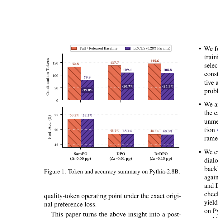
The headline results are substantial: on Pythia-2.8B, mean continuation length falls by 20.73% under DPO, 25.29% under DrDPO, and 39.84% when continuing from SamPO. On Qwen2.5-3B, reductions are 14.87% and 17.58%. Only 0.24–0.28% of parameters are updated.

2. Prerequisites

2.1 Autoregressive cost and length bias

For prompt $x$ and continuation $y=(y_1,ldots,y_T)$, an autoregressive policy factorizes as

$$\pi_\theta(y\mid x)=\prod_{t=1}^{T}\pi_\theta(y_t\mid x,y_{<t}).$$

Taking logs turns the product into a sum:

$$\log \pi_\theta(y\mid x)=\sum_{t=1}^{T}\log \pi_\theta(y_t\mid x,y_{<t}).$$

This matters twice. First, generation cost grows approximately with $T$. Second, sequence-level preference scores aggregate token-level log probabilities, so response length can interact with the optimization signal. A preference label says which answer is preferred; it does not prove that every extra token is useful.

A simple serving approximation is

$$C_{\mathrm{decode}}(T)\approx T,C_{\mathrm{step}},\qquad M_{\mathrm{KV}}(T)\approx T,m_{\mathrm{token}}.$$

The coefficients depend on batching, attention implementation, and model architecture, but the linear dependence explains why behavioral concision is a systems variable.

2.2 Pairwise preference optimization

A training example is $(x,y_w,y_l)$, where $y_w$ is preferred and $y_l$ is rejected. DPO defines an implicit reward relative to a reference policy:

$$r_\theta(x,y)=\beta\log\frac{\pi_\theta(y\mid x)}{\pi_{\mathrm{ref}}(y\mid x)}.$$

The pairwise margin is

$$m_\theta=r_\theta(x,y_w)-r_\theta(x,y_l),$$

and the DPO loss is

$$\mathcal{L}_{\mathrm{DPO}}(\theta) =-\mathbb{E}_{\mathcal D}\left[\log\sigma(m_\theta) \right].$$

The derivation is intuitive. If the policy assigns a larger reference-adjusted probability to $y_w$, then $m_\theta>0$, $\sigma(m_\theta)$ approaches one, and the loss falls. The temperature $\beta$ controls departure from the reference. LOCUS does not add a term such as $\lambda |y|$ to this objective.

DrDPO replaces an arithmetic aggregation of per-example losses by a robust log-sum-exp form. For microbatch losses $\ell_i(\theta)$,

$$\mathcal{L}_{\mathrm{DrDPO}}(\theta) =-\beta'\log\left( \frac{1}{B}\sum_{i=1}^{B}e^{-\ell_i(\theta)/\beta'} \right).$$

Factoring out the hardest loss shows why small $\beta'$ emphasizes adverse examples:

$$-\beta'\log\sum_i e^{-\ell_i/\beta'} \longrightarrow \min_i \ell_i \quad\text{as }\beta'\to 0^+,$$

up to the constant from $1/B$. LOCUS preserves this native robust objective too.

2.3 Low-rank adaptation

For a linear map with frozen weight $W_0\in\mathbb{R}^{d_1\times d_2}$, LoRA writes

$$W=W_0+\Delta W =W_0+\frac{\alpha}{r}BA,$$

where $B\in\mathbb{R}^{d_1\times r}$, $A\in\mathbb{R}^{r\times d_2}$, and $r\ll\min(d_1,d_2)$. Because $\operatorname{rank}(BA)\le r$, training is confined to a structured subset of all matrix updates.

The obvious alternative is full-parameter fine-tuning. It offers $d_1d_2$ free entries, whereas LoRA exposes only $r(d_1+d_2)$ factor entries. The restriction is useful only if the task-relevant update can be represented in that subspace. A too-small rank can underfit or—importantly for this paper—move behavior in the wrong direction.

The initialization $B=0$ and random $A$ makes $\Delta W=0$ at step zero. Thus adaptation begins exactly at the backbone function rather than with a random behavioral jump.

2.4 Utility is a proxy, not human judgment

LOCUS defines utility as chosen-versus-rejected sequence log-probability accuracy:

$$Q_t(c)=\frac{1}{|\mathcal D_t|} \sum_{(x,y_w,y_l)\in\mathcal D_t} \mathbf{1}\!\left[ \pi_c(y_w\mid x)>\pi_c(y_l\mid x) \right].$$

This metric is reproducible and cheap. It is not an external judge of factuality, safety, or answer completeness. A central theme of my critique will be that preserving this diagnostic is weaker than preserving user-visible quality.

3. LOCUS architecture and data flow

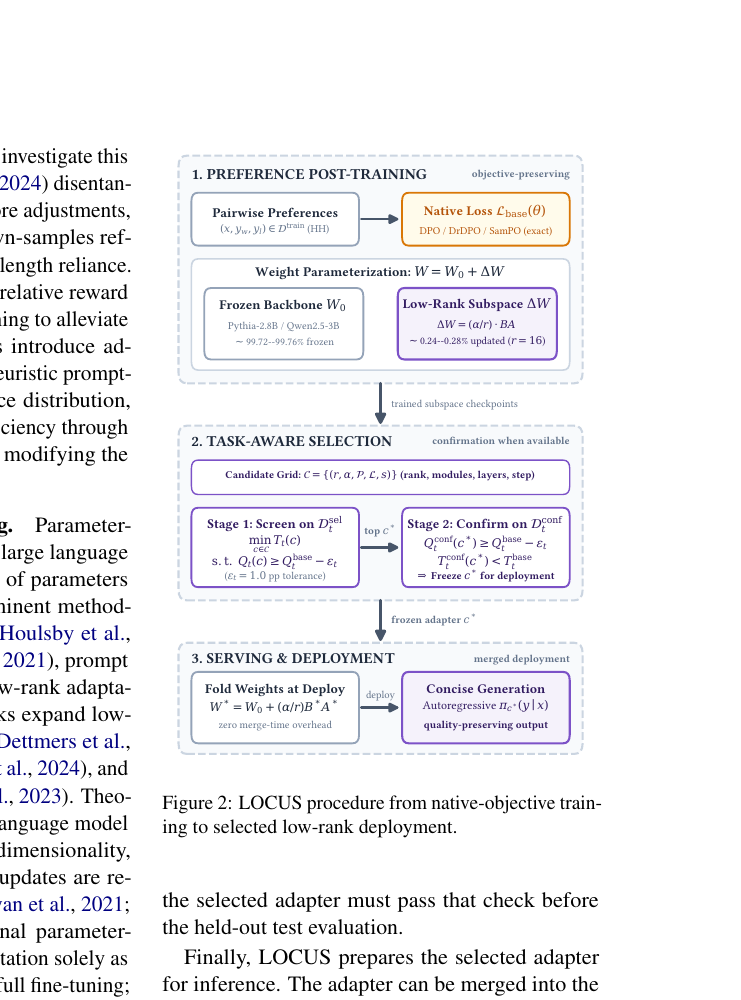
The pipeline has three stages:

1. Objective-preserving training: freeze $W_0$ and train low-rank factors using the unchanged preference objective.
2. Task-aware selection: search candidate subspaces and checkpoints on held-out development data.
3. Deployment: freeze the winner and either merge its update into the backbone or retain it as a task adapter.

The important separation is between learning and selection. The training loss never sees a token penalty. Length enters only when choosing among already-trained candidates. This avoids directly teaching the model that termination is always good, but it shifts responsibility to the validation protocol.

3.1 Candidate configuration

A candidate is the tuple

$$c=(r,\alpha,\mathcal P,\mathcal L,s)\in\mathcal C,$$

where $r$ is adapter rank, $\alpha$ is scaling, $\mathcal P\subseteq{Q,K,V,O,\mathrm{MLP}}$ chooses projections, $\mathcal L$ chooses layers, and $s$ is a training checkpoint. This definition makes time part of the search space: two checkpoints from the same adapter trajectory can have different length–utility behavior.

For task $t$, let $T_t(c)$ be mean continuation tokens under greedy decoding. LOCUS solves

$$c_t^*=\arg\min_{c\in\mathcal C}T_t(c)$$

subject to

$$Q_t(c)\ge Q_t^{\mathrm{base}}-\epsilon_t, \qquad \epsilon_t=1.0\text{ percentage point}.$$

Geometrically, each candidate is a point $(T,Q)$. The constraint discards points below a horizontal utility floor; the objective picks the leftmost surviving point. This is a constrained Pareto decision, not a scalarized loss.

3.2 Algorithm 1 — train, screen, confirm

Numbered pseudocode

1. Evaluate baseline utility $Q_{\mathrm{base}}^{\mathrm{sel}}$ on the selection split.
2. For every configuration $c\in\mathcal C$, train $\Delta W_c$ from the designated starting checkpoint with the native objective.
3. Generate on the selection prompts; record mean tokens $T^{\mathrm{sel}}(c)$ and utility $Q^{\mathrm{sel}}(c)$.
4. Form the feasible set
   $\mathcal C_{\mathrm{feas}}={c:Q^{\mathrm{sel}}(c)\ge Q_{\mathrm{base}}^{\mathrm{sel}}-\epsilon}$.
5. If the set is empty, return the baseline.
6. Select $c^*=\arg\min_{c\in\mathcal C_{\mathrm{feas}}}T^{\mathrm{sel}}(c)$.
7. If no confirmation split exists, label $c^*$ unconfirmed and stop.
8. Otherwise evaluate $c^*$ and the baseline on the disjoint confirmation split.
9. Accept only if $Q^{\mathrm{conf}}(c^*)\ge Q_{\mathrm{base}}^{\mathrm{conf}}-\epsilon$ and $T^{\mathrm{conf}}(c^*)<T_{\mathrm{base}}^{\mathrm{conf}}$.
10. If either test fails, deploy the baseline; otherwise freeze $c^*$.

Why confirmation? Searching many candidates selects partly on noise. Rechecking one winner on untouched data reduces this winner’s-curse effect. The obvious alternative—selecting and reporting on one development split—would overstate robustness. The remaining boundary is that two sets of only 256 examples can still have wide uncertainty.

3.3 Algorithm 2 — compute the utility diagnostic

Although simple, the diagnostic is another key algorithm because every feasibility decision depends on it.

1. For each pair $(x,y_w,y_l)$, teacher-force the model on $y_w$ and sum token log probabilities.
2. Teacher-force on $y_l$ in exactly the same way.
3. Record one if $\log\pi_c(y_w\mid x)>\log\pi_c(y_l\mid x)$, else zero.
4. Average these indicators across the split.
5. Report the value with the split identity; never mix selection, confirmation, and test values.

Summing token log probabilities rather than averaging them leaves a residual length interaction. Longer strings accumulate more negative log-probability terms. This makes the diagnostic protocol-reproducible but not length-neutral, a subtle issue the paper does not fully resolve.

4. Why can the parameterization change verbosity?

Low-rank adaptation does not contain a built-in “be concise” axis. The mechanism is indirect. Factorization changes optimization geometry: gradients with respect to $A$ and $B$ are coupled through their product. For a scalar loss $\mathcal L$ and $G=\partial\mathcal L/\partial W$,

$$\frac{\partial\mathcal L}{\partial B} =\frac{\alpha}{r}GA^\top, \qquad \frac{\partial\mathcal L}{\partial A} =\frac{\alpha}{r}B^\top G.$$

An infinitesimal factor update induces

$$d(\Delta W)=\frac{\alpha}{r}(dB,A+B,dA).$$

Therefore the reachable first-order direction lies in the tangent space around the current factor pair, rather than the entire $d_1d_2$ matrix space. Different ranks and placements expose different tangent directions; checkpoint selection samples different points along those trajectories.

4.1 Parameter-count proposition, derived carefully

Full fine-tuning of one $d_1\times d_2$ matrix exposes

$$N_{\mathrm{full}}=d_1d_2$$

trainable scalars. LoRA stores two factors, so

$$N_{\mathrm{LoRA}}=d_1r+rd_2=r(d_1+d_2).$$

LoRA uses fewer exposed entries exactly when

$$r(d_1+d_2)<d_1d_2,$$

or equivalently

$$r<\frac{d_1d_2}{d_1+d_2}.$$

For a square $d\times d$ projection this becomes $r<d/2$. With $d=2560$ and $r=16$:

$$N_{\mathrm{full}}=2560^2=6{,}553{,}600,$$ $$N_{\mathrm{LoRA}}=16(2560+2560)=81{,}920,$$

a factor-entry reduction of $80\times$ for that matrix.

This count is not the intrinsic dimension of rank-$r$ matrices. For any invertible $G\in\mathbb R^{r\times r}$,

$$(BG)(G^{-1}A)=BA.$$

The $r^2$-dimensional change-of-basis redundancy means the rank-$r$ manifold has local dimension

$$r(d_1+d_2-r),$$

at full-rank factors. Optimizers still maintain entries and states for all $r(d_1+d_2)$ factor coordinates, so the implementation count and geometric dimension answer different questions.

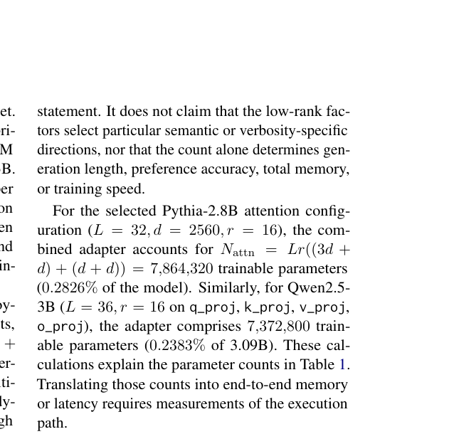
For Pythia’s 32 layers with fused QKV and output projections, the paper gives

$$N_{\mathrm{attn}} =32\cdot16\left[(3d+d)+(d+d) \right] =7{,}864{,}320$$

at $d=2560$, or 0.2826% of the model. Qwen2.5-3B uses separate grouped-query projections and totals 7,372,800 entries, 0.2383%.

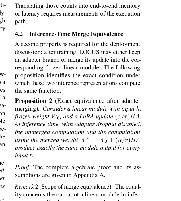
4.2 Algorithm 3 — merge an adapter for serving

1. Disable adapter dropout and switch the module to inference mode.
2. Load frozen $W_0$ and trained factors $A^*,B^*$.
3. Compute the update $\Delta W=(\alpha/r)B^*A^*$ in an appropriate accumulation dtype.
4. Form $W^*=W_0+\Delta W$.
5. Replace the two-branch module with the single linear map $hmapsto W^*h+b$.
6. Validate logits within the numerical tolerance appropriate to the dtype or quantizer.
7. Retain the unmerged factors as the recoverable source artifact.

The exact real-arithmetic proof is short:

$$z_{\mathrm{unmerged}} =W_0h+\frac{\alpha}{r}B(Ah)+b,$$ $$z_{\mathrm{unmerged}} =\left(W_0+\frac{\alpha}{r}BA \right)h+b =W^*h+b =z_{\mathrm{merged}}.$$

Associativity and distributivity prove equality for every $h$. The boundary conditions matter: dropout must be off; quantization and finite-precision reordering can produce small differences; and a multi-tenant server may intentionally keep adapters unmerged.

4.3 Design choice: selection instead of length regularization

Why it works: the native objective remains comparable with its baseline, while validation chooses an operating point with lower token cost.

Obvious alternative: add $\lambda T$ to the training loss or reward. This directly pushes toward shorter outputs and needs only one model.

Where LOCUS can fail: the candidate grid is expensive, validation utility is imperfect, and a model may learn abrupt or incomplete answers that happen to pass the internal preference test. Selection does not eliminate Goodhart’s law; it changes which metric is optimized at which stage.

4.4 Design choice: attention-only adapters

The selected configuration applies LoRA to attention projections. This is not universally optimal, but the ablation shows a favorable parameter–reduction trade-off. Attention-All obtains 15.95% reduction with 7.86M trainable entries; All-Linear obtains 13.88% despite 20.97M.

The obvious alternative is to adapt every linear layer. It increases expressive power but also changes optimization geometry and triples adapter size. MLP-only adaptation reaches only 5.75% in the reported screen. The boundary is model architecture: fused QKV in Pythia and grouped-query attention in Qwen expose different shapes, so “same target family” is not the same subspace.

5. Experimental design

5.1 Backbones, data, and baselines

The paper evaluates Pythia-2.8B (32 GPT-NeoX layers, hidden size 2560) and Qwen2.5-3B (36 Llama-style layers, hidden size 2048, GQA, SwiGLU, RMSNorm). All runs use one NVIDIA A100 PCIe 80 GB in bfloat16. Full-parameter DPO and DrDPO use activation checkpointing and 512-token sequences.

The primary corpus is Anthropic Helpful and Harmless. Controlled DPO/DrDPO comparisons share the same full-parameter SFT starting checkpoint, training pool, objective, and split. This matching is essential: comparing a LoRA branch against an unrelated released model would confound parameterization with data and initialization.

Primary held-out evaluation uses 8,552 HH pairs. Selection and confirmation each use 256 examples where specified. SamPO follows its established 256-example split and starts from the official checkpoint, so it is a continuation experiment rather than a same-SFT controlled comparison.

Generation uses greedy decoding with sampling disabled and at most 256 new tokens. Continuation tokens exclude EOS, and limit hits are recorded. Greedy decoding improves reproducibility but says nothing about the sampling regimes common in chat products.

5.2 Checkpoint selection

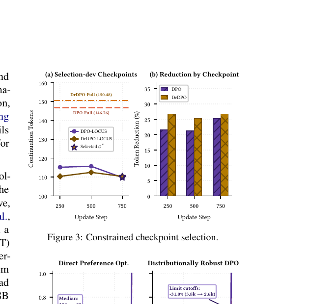
LOCUS evaluates 250-, 500-, and 750-step checkpoints. Length trajectories are non-monotonic, so “train longer” is not a valid selection rule. For Pythia DPO and DrDPO, the utility-constrained procedure ultimately chooses step 750.

This design makes early stopping task-aware. Conventional early stopping minimizes validation loss, which may not align with either token cost or the chosen-versus-rejected diagnostic. LOCUS instead stops at a behavioral operating point. The cost is multiple generations for every candidate.

5.3 Main Pythia results and distribution shape

Objective	Baseline tokens	LOCUS tokens	Reduction	Preference accuracy delta
SamPO	132.77	79.88	39.84%	0.00 pp
DPO	137.67	109.12	20.73%	-0.01 pp
DrDPO	145.61	108.79	25.29%	-0.13 pp

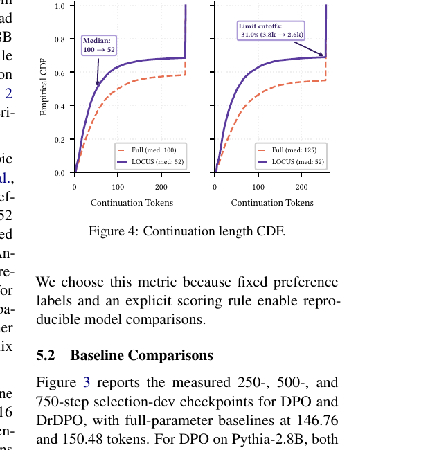
For DPO, the median falls from 100 to 52 tokens. For DrDPO, it falls from 125 to 52. Limit hits fall by 24.70% and 30.98%, respectively. These distributional statistics strengthen the claim: a lower mean could otherwise be caused by shortening only a handful of extreme responses.

A practical cost translation is

$$\text{decode savings}\approx N_{\mathrm{requests}} (T_{\mathrm{base}}-T_{\mathrm{LOCUS}}) C_{\mathrm{step}}.$$

For one million DPO requests, the measured difference is

$$10^6(137.67-109.12)=28.55\text{ million decoded tokens}.$$

This is not a direct dollar estimate because batching, memory bandwidth, and hardware utilization are unreported. It does show why a behavioral reduction can matter at fleet scale.

5.4 Rank sensitivity: low rank is not monotonic magic

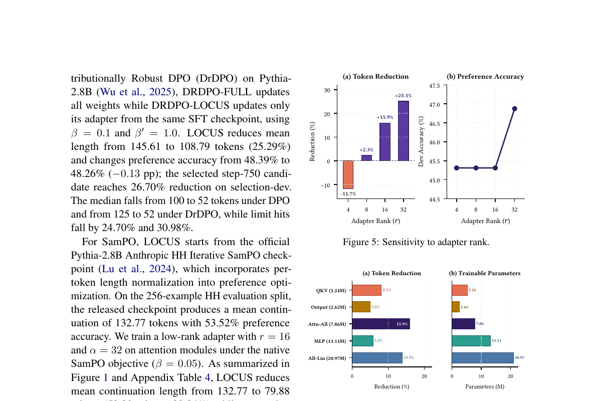
With fixed attention placement and $\alpha/r=2$, ranks $4,8,16,32$ yield token reductions of approximately $-11.74\%$, $2.32\%$, $15.95\%$, and $25.10\%$. The negative reduction at rank 4 means length inflation.

This is one of the paper’s most informative results. If parameter efficiency alone caused concision, the smallest rank should work best. It does not. Rank changes the reachable update geometry; below a threshold, the model may represent preference cues but not the decision boundary that ends an answer cleanly.

The internal preference diagnostic remains 45.31% at ranks 4, 8, and 16 and rises to 46.88% at rank 32. Since token reduction changes dramatically while this diagnostic barely changes, the adapter can move along a behavioral dimension largely invisible to the reported utility metric.

5.5 Target-module ablation

Target set	Trainable parameters	Token reduction
Fused QKV only	5.24M	8.09%
Attention output only	2.62M	4.96%
Attention-All	7.86M	15.95%
MLP	13.11M	5.75%
All-Linear	20.97M	13.88%

The ablation refutes a capacity-only explanation. All-Linear has 2.7 times the trainable entries of Attention-All yet a smaller reduction. Placement matters because attention projections directly influence token-to-token information flow and next-token logits; adding MLP freedom may open trajectories that preserve verbosity.

5.6 Cross-task and cross-backbone transfer

Pythia DPO reductions are 20.73% on HH dialogue, 25.29% on the Harmless development set, and 79.97% on Orca DPO development data. The corresponding preference diagnostic changes are -0.01, +1.17, and +13.67 percentage points.

The 79.97% Orca result is striking but should not be read as a held-out quality claim. It uses 256 development examples. It may reflect task structure, baseline verbosity, or selection overfit. The paper properly labels this scope, though the headline visual invites casual overgeneralization.

On Qwen2.5-3B, controlled DPO drops from 108.26 to 92.16 tokens (14.87%) with -0.05 pp diagnostic change. DrDPO drops from 111.58 to 91.97 (17.58%) with -0.09 pp. This cross-family evidence is useful, but both backbones remain around 3B parameters.

6. A worked example of constrained selection

Suppose a baseline has $Q_{\mathrm{base}}=49.0\%$ and mean length 140. With $\epsilon=1.0$ pp, the utility floor is 48.0%.

Candidate	Rank	Targets	Step	Utility	Tokens	Feasible?
A	4	Attention	250	49.2%	151	yes
B	8	Attention	500	48.7%	126	yes
C	16	Attention	750	48.3%	104	yes
D	32	All-Linear	750	47.5%	82	no

Candidate D is shortest but violates the constraint. LOCUS selects C. On confirmation, imagine C obtains 47.8% while the baseline obtains 49.1%. Since

$$47.8\% < 49.1\%-1.0\%=48.1\%,$$

the adapter fails and the system returns the baseline. This fallback is a meaningful safety valve. It also shows that LOCUS optimizes a relative utility tolerance: a weak baseline sets a weak floor.

6.1 Statistical uncertainty

For a binary accuracy over $n=256$ examples with observed proportion $\hat p\approx0.5$, the standard error is approximately

$$\operatorname{SE}(\hat p) =\sqrt{\frac{\hat p(1-\hat p)}{n}} \approx\sqrt{\frac{0.25}{256}} =3.125\text{ percentage points}.$$

A rough 95% interval is about $pm6.1$ pp, much wider than the 1 pp tolerance. Paired comparisons can reduce uncertainty because baseline and candidate score the same examples, but the paper does not report paired confidence intervals or hypothesis tests for feasibility.

For mean length, heavy tails and the hard 256-token cap complicate a Gaussian approximation. A paired bootstrap over prompts would preserve baseline–candidate correlation:

1. Sample 256 prompt indices with replacement.
2. Compute the paired mean length difference and utility difference.
3. Repeat, for example, 10,000 times.
4. Accept only if the desired quantile satisfies both constraints.

This turns the deterministic feasibility test into a risk-controlled decision.

6.2 Algorithm 4 — uncertainty-aware LOCUS extension

1. Train and evaluate candidates exactly as in Algorithm 1.
2. For each candidate, bootstrap paired prompt outcomes.
3. Estimate a lower confidence bound $L_Q(c)$ for utility difference and an upper bound $U_T(c)$ for token difference.
4. Define feasibility by $L_Q(c)\ge-\epsilon$ and $U_T(c)<0$.
5. Among feasible candidates, minimize expected tokens or a high quantile of tokens.
6. Confirm the winner on untouched data using the same paired procedure.
7. Fall back to the baseline if either confidence condition fails.

This extension costs no additional model training; it uses the already-generated evaluation data. Its limitation is that bootstrap validity still assumes the prompt sample represents deployment traffic.

7. Systems interpretation

7.1 Training memory is not just parameter count

For Adam with two moment states, trainable parameters, gradients, and optimizer states scale with $N_{\mathrm{train}}$. A rough mixed-precision accounting is

$$M_{\mathrm{trainable}} \approx N_{\mathrm{train}} (b_{\mathrm{param}}+b_{\mathrm{grad}}+b_{m}+b_v).$$

If parameters and gradients use 2 bytes and moments use 4 bytes each, this is roughly 12 bytes per trainable entry before master weights and framework overhead. For 7.86M entries, that component is about 94 MB. Full fine-tuning of 2.8B entries is tens of gigabytes for the analogous states.

However, freezing the backbone does not remove forward activations or all backward computation. Gradients must propagate through frozen layers to reach adapters. The paper is careful not to claim end-to-end memory or speed improvements from parameter count alone.

7.2 Inference trade-offs

Merged single-tenant deployment adds no LoRA branch at runtime. Multi-tenant serving is different: keeping one backbone and many adapters saves duplicated backbone memory, but adapter selection, memory movement, and extra matrix multiplications remain.

A simplified unmerged projection computes

$$Wh=W_0h+\frac{\alpha}{r}B(Ah).$$

The adapter FLOPs per token scale as

$$C_{\mathrm{adapter}}\propto r(d_1+d_2),$$

which is small compared with $d_1d_2$ for low rank, but not zero. Whether shorter sequences outweigh adapter overhead depends on batch size, rank, kernel fusion, and cache behavior. The paper measures token reduction, not serving throughput or p99 latency.

8. Reproducibility blueprint

The paper gives useful protocol details: model families, layer shapes, adapter parameter counts, datasets, split sizes, objectives, beta values, checkpoint steps, hardware, precision, maximum generation length, and greedy decoding. A careful reproduction should lock all of them.

8.1 Algorithm 5 — minimal reproducible experiment

1. Materialize immutable train, selection, confirmation, and test manifests with example IDs.
2. Train one shared SFT checkpoint from the stated HH pool.
3. Clone that checkpoint into a full-parameter branch and a LoRA branch.
4. For DPO, set $\beta=0.1$; for DrDPO, additionally set $\beta'=1.0$.
5. Attach rank-16, $\alpha=32$ adapters to all attention projections.
6. Train candidate checkpoints at steps 250, 500, and 750 with matched data order and decoding protocol.
7. Evaluate every candidate on selection data with greedy decoding and 256 new-token cap.
8. Apply the one-percentage-point utility constraint and choose the shortest candidate.
9. Confirm on the disjoint 256-pair split.
10. Freeze the selected configuration before touching the 8,552-pair test set.
11. Report paired mean, median, cutoff-hit rate, and preference diagnostic.
12. Save generated continuations so independent reviewers can inspect truncation and completeness.

8.2 Audit checklist

• Verify that token counts exclude EOS consistently.
• Verify whether prompts contribute to sequence log probability; only continuations should differ.
• Confirm tokenizer identity between full and low-rank branches.
• Use identical stopping criteria and chat templates.
• Report random seeds and candidate multiplicity.
• Keep the SamPO continuation result separate from same-SFT controlled comparisons.
• Compare generated answer correctness with at least one external evaluator and human sample.
• Measure wall-clock tokens/s, time-to-first-token, inter-token latency, peak memory, and p99 latency.
• Test sampled decoding at multiple temperatures.
• Inspect how often shorter answers omit required caveats or steps.

8.3 Expected failure signatures

A reproduction can fail without a code bug. Rank 4 may inflate length, as the paper observes. A selected candidate may pass selection and fail confirmation. A module set that works on Pythia may not map cleanly to Qwen because QKV layouts differ. Quantized merging may violate bitwise equivalence even when float arithmetic is algebraically identical.

The correct response is not to tune on the test set. Expand or redesign the candidate grid using development data, then preserve a fresh final evaluation.

9. Limitations and boundary conditions

The authors acknowledge several important boundaries:

1. Only two decoder-only backbones near 3B parameters are tested.
2. Generation is greedy; stochastic sampling remains untested.
3. Candidate ranks are discrete and module groupings coarse.
4. Fine-grained layer selection, continuous rank allocation, and gradient-informed pruning are absent.
5. Cross-task safety and instruction-following rows are development evaluations.
6. Parameter reduction is not a demonstrated end-to-end training or serving speedup.

Additional technical boundaries follow from the method.

Metric boundary. Chosen-versus-rejected log-probability accuracy is an internal diagnostic. It can remain constant while factuality, calibration, style, or completeness changes.

Search-cost boundary. Training several candidates can cost more aggregate compute than training one full model, even if each adapter is cheap. The paper does not provide search-budget accounting.

Traffic boundary. Mean token length on HH prompts may poorly predict production traffic with tools, retrieval, code, multilingual prompts, or long reasoning tasks.

Baseline boundary. The constraint protects relative utility. If the baseline is poor or already length-biased, LOCUS preserves only that protocol-specific reference point.

Termination boundary. A 256-token cap censors the right tail. Fewer cap hits are encouraging, but capped means do not reveal how long uncensored generations would have been.

Causal boundary. Results show that selected low-rank trajectories correlate with concision. They do not identify a semantic subspace for verbosity or prove that low rank is the cause independent of optimization and early stopping.

10. Critical Analysis

10.1 Paper-specific weaknesses and flaws

The largest weakness is the mismatch between the strength of the claim—utility-preserving generation—and the narrow utility measurement. Preference accuracy around 48–53% is both close to chance and nearly unchanged. It is unclear whether this diagnostic is sensitive enough to detect degraded answers. The paper demonstrates preservation of an internal ranking statistic, not preservation of user utility.

The second weakness is statistical. Selection and confirmation use 256 examples, yet the acceptance tolerance is only one percentage point. Around 50% accuracy, a naive binomial standard error exceeds three percentage points. Without paired uncertainty intervals, “within one point” appears more precise than the sample supports.

Third, the search budget is missing. LOCUS trains candidates over rank, scaling, placement, layer scope, and checkpoint. Reporting only the winning adapter’s parameter count makes deployment look cheap while hiding the offline cost required to find it.

Fourth, the SamPO comparison is easy to misread. LOCUS continues from an official SamPO checkpoint, whereas controlled DPO and DrDPO compare branches from shared SFT checkpoints. The 39.84% result is valuable, but it is not evidence that LOCUS beats a protocol-matched full-parameter SamPO run.

Fifth, the paper contains no human or external quality evaluation of generated continuations. Examples of shortened outputs would make failure modes visible. Mean length and pairwise probability accuracy cannot reveal whether a response stopped after the answer or before the explanation.

10.2 Limitations that are understated or omitted

The multiple-comparisons problem is understated. Searching many candidate configurations and checkpoints against one selection set increases the probability of a lucky short candidate. One confirmation split helps, but the exact number of attempted candidates should be reported and uncertainty corrected.

The interaction between sequence length and the utility metric deserves deeper treatment. Sequence log probability is a sum across tokens; comparing raw sequence probabilities can itself favor shorter strings. If the feasibility metric is length-sensitive, the constraint may not be independent of the optimization target.

The method may shift costs rather than remove them. A concise answer that triggers more user follow-ups can increase total conversation tokens. Request-level length should be complemented by task-completion and multi-turn cost.

Safety tasks can require detailed refusals, and reasoning tasks can require verifiable intermediate steps. A universal pressure toward shorter outputs is inappropriate. LOCUS is task-specific, but deployment safeguards for tasks with minimum explanation requirements are not discussed.

Finally, exact merge equivalence is an algebraic property already known for LoRA. It is useful documentation but should not be interpreted as empirical evidence of systems speedup.

10.3 Concrete improvement suggestions

1. Add blind human evaluation of correctness, completeness, harmfulness, and unnecessary verbosity.
2. Use paired bootstrap confidence bounds in the feasibility rule.
3. Report the complete candidate grid, all failed candidates, seeds, and aggregate GPU-hours.
4. Add length-normalized and calibrated preference diagnostics alongside raw sequence accuracy.
5. Evaluate 7B–70B models, multilingual prompts, tool use, code, and long-form reasoning.
6. Test temperature and nucleus sampling, not only greedy decoding.
7. Publish prompt-level generations and annotate why each shorter answer is or is not sufficient.
8. Measure end-to-end throughput, p50/p99 latency, energy, KV-cache occupancy, and multi-turn total tokens.
9. Compare with a matched length-regularized objective and a simple checkpoint-selection baseline.
10. Use per-task lower and upper length constraints so concision cannot collapse necessary reasoning.
11. Evaluate cross-task adapter transfer without reselection to separate general subspaces from task-specific search.
12. Pre-register the utility tolerance and candidate budget before final testing.

11. What I learned

The paper’s strongest idea is conceptual: parameter-efficient tuning is not merely an approximation to full fine-tuning. Its geometry can change behavior even when the loss, data, and starting point are fixed. Rank and placement become knobs for navigating a length–utility frontier.

Its strongest evidence is not the maximum reduction; it is the collection of controls. Shared-SFT DPO and DrDPO branches, rank sensitivity, module ablation, distributional length plots, and a second backbone jointly rule out several simple explanations.

Its weakest link is measurement. “Utility-preserving” should be read as “preserving the reported chosen-versus-rejected diagnostic within the tested protocol.” That narrower claim is still interesting and operationally relevant.

12. Conclusion

LOCUS trains low-rank adapters under unchanged preference objectives and selects the shortest utility-feasible configuration. On two roughly 3B backbones it reduces mean continuation length by 14.87–39.84% while updating under 0.3% of parameters. Adapter rank and placement matter non-monotonically, and merged deployment is algebraically equivalent to the unmerged linear computation.

For practitioners, the method is a promising validation-time wrapper around PEFT: define a candidate grid, preserve the native objective, screen on token cost, confirm on untouched data, and retain a baseline fallback. Before production adoption, however, I would require stronger utility evaluation, uncertainty-aware selection, full search-cost reporting, sampled decoding, and direct serving measurements.

The broader lesson is useful: optimization subspaces are behavioral controls. But a behavioral control is only as trustworthy as the metric and validation design that select it.