KV-Pipe: Turning a KV-Cache Trick Into a Pipeline-Parallel Load Balancer

Review date: 2026-08-23 Author: Zhongzhu Zhou Paper reviewed: KV-Pipe: On the Relation Between KV Sharing and Pipeline Parallel Efficiency in LLMs Paper authors: Maryam Dialameh, Hossein Rajabzadeh, Harish Krishnamoorthy Murali, Walid Ahmed, Weiwei Zhang, Hyock Ju Kwon (University of Waterloo & Huawei Ascend Team, Toronto) arXiv: 2608.15943 Venue/Status: Preprint (cs.DC), August 2026

1. The idea in one sentence, and why it’s not obvious

Cross-layer KV sharing is a well-worn trick: instead of every attention layer projecting and caching its own keys and values, some layers reuse the $(K, V)$ tensors computed by an earlier layer. It shows up in the literature almost exclusively as an inference-time memory-compression technique — smaller KV cache, less redundant projection work, faster decoding at long context lengths. KV-Pipe’s contribution is to notice that the same mechanical change — converting a full-attention layer into a KV-sharing layer — also shrinks that layer’s FLOPs, and FLOPs per layer is exactly the quantity that determines how evenly a pipeline-parallel (PP) training run is balanced across stages. If one pipeline stage happens to be your bottleneck because it’s carrying disproportionately expensive layers (or an extra module like the LM head), you can selectively convert that stage’s layers to KV-sharing and shrink its compute until it stops being the bottleneck — all without touching the training schedule, the optimizer, the parallelism degree, or model correctness assumptions in a way that requires re-architecting anything.

That’s the whole idea. It’s a small idea, and the paper is honest that none of its individual pieces (KV sharing, pipeline imbalance, greedy bottleneck reduction) are new in isolation. What’s genuinely useful is the connection: nobody had previously used a KV-cache compression technique as a load-balancing lever for pipeline-parallel training, and once you see it, the empirical payoff (3–9% MFU gains, composable with existing pipeline schedulers, and a bonus inference-time speedup from the same converted layers) is a clean demonstration that “memory-side” and “compute-side” optimizations for a Transformer are not actually separate design spaces — they’re two views of the same per-layer cost profile.

This review is aimed at a reader who knows what pipeline parallelism and KV caching are individually, but hasn’t seen anyone connect the two. Section 2 builds the prerequisites (pipeline parallelism and its bubble problem; the mechanics of cross-layer KV sharing) from first principles. Sections 3–4 unpack KV-Pipe’s core metric and algorithm step by step, including the full pseudocode. Section 5 walks through every experiment in the paper, not just the headline numbers. Section 6 covers limitations, and Section 7 is a dedicated critical-analysis section — the paper’s honesty about its own scope is one of its more admirable qualities, and it’s worth taking seriously rather than skimming past.

2. Prerequisites

2.1 Pipeline parallelism and the bubble problem

When a Transformer model is too large to fit (parameters, activations, optimizer state) on a single accelerator, one standard solution is pipeline parallelism (PP): partition the model’s $L$ layers into $P$ contiguous groups (“stages”), and place each stage on a different device. A training micro-batch flows through the stages in sequence during the forward pass, and back through them in reverse during the backward pass — much like an assembly line, where each worker (device) performs one step of the process and passes the (partially processed) item to the next worker.

The efficiency problem with a naive pipeline is immediate: if you send a single micro-batch through the pipeline, only one device is ever active at a time — the other $P - 1$ devices sit idle waiting for their turn, an obviously terrible utilization story. The standard fix, introduced by GPipe (Huang et al., 2019) and refined by PipeDream (Narayanan et al., 2019) and its 1F1B (“one-forward-one-backward”) scheduling variant, is to split each training step into many small micro-batches and pipeline them: while device 2 works on micro-batch 1’s forward pass, device 1 can already start micro-batch 2’s forward pass. This overlaps computation across devices and dramatically improves utilization — but it does not eliminate idle time entirely. At the start of the pipeline (filling it with micro-batches) and the end (draining it), some devices are necessarily idle; this idle time is called a pipeline bubble. The 1F1B schedule (used as the primary baseline throughout this paper) reduces bubble time and peak activation memory relative to GPipe’s naive “all-forward-then-all-backward” schedule, but it does not solve a second, more insidious source of idle time: stage imbalance.

Stage imbalance means: even with a perfect scheduling algorithm that eliminates every avoidable bubble, if stage 3 takes twice as long to compute its forward+backward pass as stage 1, then stage 1 will unavoidably sit idle waiting for stage 3 on every pipeline step, because the pipeline as a whole can only advance as fast as its slowest stage — a direct architectural analogue of Amdahl’s law applied to an assembly line. The naive assumption behind pipeline parallelism is that if you split $L$ identical Transformer blocks into $P$ equal-sized groups, each stage does roughly $L/P$ of the total work and stages are naturally balanced. In practice this assumption is frequently false, for reasons the paper is careful to spell out:

• Non-uniform auxiliary modules. The embedding layer typically lives on stage 1, and the final LM projection head (“LM head”) typically lives on stage $P$ — but the LM head, especially for large vocabularies, can add substantial extra FLOPs to whichever stage holds it, meaning the last stage is structurally heavier even if every attention layer were identical.
• Heterogeneous attention variants. Modern LLMs increasingly mix full attention with cheaper variants (sliding-window attention, in models like Mistral), so a “stage” containing more full-attention layers costs more than one containing more windowed-attention layers.
• Sparse MoE layers. Mixture-of-Experts layers change per-layer parameterization and token-wise compute in ways that are not uniform across depth.
• Hybrid architectures. Transformer–Mamba hybrids (Jamba, Nemotron-H) interleave fundamentally different sequence-modeling blocks with different costs per layer.

A large body of prior systems work attacks this problem from the scheduling or placement side: re-partitioning layers across stages to balance memory and compute (BPipe, DawnPiper), filling bubble time with unrelated work (PipeFill), or handling prefill/decode heterogeneity during serving with phase-aware batching (Sarathi-Serve, gLLM, TD-Pipe, Seesaw). What all of these approaches share is that they treat the per-layer cost profile as a fixed input and try to place it well or hide its consequences. KV-Pipe’s angle is different: instead of accepting the per-layer cost profile as given, it directly changes it by converting selected layers to a cheaper attention variant.

2.2 Cross-layer KV sharing, mechanically

In a standard (“full attention”) Transformer decoder layer $\ell$, given hidden states $X_\ell \in \mathbb{R}^{S \times d}$ (sequence length $S$, hidden dimension $d$), the layer computes its own query, key, and value projections:

$$Q_\ell = X_\ell W_\ell^Q, \quad K_\ell = X_\ell W_\ell^K, \quad V_\ell = X_\ell W_\ell^V, \tag{1}$$

and then attention output

$$O_\ell = \mathrm{softmax}\!\left(\frac{Q_\ell K_\ell^\top}{\sqrt{d_h}} + M\right) V_\ell, \tag{2}$$

where $M$ is the causal mask (preventing a token from attending to future tokens) and $d_h$ is the per-head dimension. During autoregressive decoding, the freshly computed $(K_\ell, V_\ell)$ pair for the new token is appended to that layer’s KV cache, so future decoding steps can reuse it without recomputation — this is standard KV caching, distinct from cross-layer sharing.

Cross-layer KV sharing goes one step further: instead of computing a fresh $(K_\ell, V_\ell)$ for layer $\ell$, the layer reuses the keys and values already computed by some earlier layer $\tau(\ell) < \ell$:

$$K_\ell \leftarrow K_{\tau(\ell)}, \qquad V_\ell \leftarrow V_{\tau(\ell)}. \tag{3}$$

Crucially, the query projection and the attention computation itself (Eq. 2) are unchanged — only the $K$/$V$ tensors are borrowed. This is the mechanism used by systems like MLKV (sharing across layers) and HShare (sharing critical KV indices across layers/heads/queries), and it has two direct, measurable effects at the layer level:

• It removes the $K_\ell$ and $V_\ell$ projection matmuls entirely for that layer (no $W_\ell^K$, $W_\ell^V$ compute), which reduces the layer’s FLOPs by an amount the paper denotes $\Delta F_\ell = F_\ell(0) - F_\ell(1)$, where $F_\ell(0)$ is the full-attention FLOPs and $F_\ell(1)$ is the KV-sharing FLOPs for layer $\ell$.
• It removes the need to store a fresh $(K_\ell, V_\ell)$ in the KV cache for that layer, reducing per-token KV-cache bytes by an amount $\Delta B_\ell$ — this is the classical inference-time benefit that motivated KV sharing in the first place.

Everything downstream in the paper follows from noticing that $\Delta F_\ell$ — the FLOPs saved by conversion — is exactly the quantity you want to control if your goal is to shrink a bottleneck pipeline stage.

2.3 Why this specific combination hadn’t been tried before

It’s worth being explicit about why “use KV sharing to balance a pipeline” is not a trivial observation, even in hindsight. Prior cross-layer KV-sharing work was developed and evaluated entirely in an inference context, where the object of interest is decode-time latency and KV-cache memory, and where there is no pipeline-stage structure to speak of (most of these systems assume tensor-parallel or single-device serving). Prior pipeline-balancing work assumed the per-layer cost profile was architecturally fixed and tried to work around it via scheduling or partition search. Bridging the two requires recognizing that KV sharing is not just a memory optimization — it is a FLOPs optimization at the layer level, and FLOPs-per-layer is the primitive that determines PP stage balance. Once you frame it that way, the idea that you can selectively apply a memory-motivated trick as a compute-balancing lever falls out naturally — but as far as the related work in this paper indicates, nobody had made that connection explicit and measured it before.

3. The core metric: FLOPs Imbalance Ratio (FIR)

Before you can balance a pipeline, you need a way to measure how unbalanced it currently is. KV-Pipe proposes a simple, interpretable metric for this: the FLOPs Imbalance Ratio (FIR).

Let $F_{\text{stage}_i}$ denote the total FLOPs assigned to stage $i$ (summing the FLOPs of every layer placed on that stage, plus any auxiliary module like the LM head if it lives there). Define

$$\mathrm{FIR} = \frac{\max_i F_{\text{stage}_i}}{F_{\text{avg}}}, \tag{4}$$

where $F_{\text{avg}}$ is the average FLOPs across all $P$ stages, computed carefully to account for architectural non-uniformity:

$$F_{\text{avg}} = \frac{1}{P}\sum_{i=1}^{P}\left(\sum_{k=1}^{N} F_{\text{stage}_i}^{\text{layer}_k} + \delta_{i,P} F_{\text{LM-Head}}\right), \tag{5}$$

where $\delta_{i,P}$ is the Kronecker delta ($\delta_{i,P} = 1$ if $i = P$, else $0$), $F_{\text{LM-Head}}$ is the FLOPs of the LM head (conventionally attached to the last stage), and $F_{\text{stage}_i}^{\text{layer}_k}$ is the FLOPs of the $k$-th layer placed on stage $i$.

Intuition and derivation walkthrough. The numerator, $\max_i F_{\text{stage}_i}$, picks out the single most expensive stage — this is the stage that determines the pipeline’s throughput ceiling, because every other stage must wait for it on every pipeline step (the bottleneck-dominates-throughput argument from Section 2.1). The denominator, $F_{\text{avg}}$, is what the bottleneck would cost if FLOPs were spread perfectly evenly across all $P$ stages. The ratio of the two tells you, in a single number, how much worse your actual bottleneck is than the theoretical best case: $\mathrm{FIR} = 1$ means every stage carries exactly the average FLOPs (perfect balance, no stage is disproportionately slow); $\mathrm{FIR} > 1$ quantifies the excess cost concentrated in the worst stage. A FIR of 1.12, for instance, means the bottleneck stage carries 12% more FLOPs than a perfectly balanced pipeline would assign it — and, to first order, you’d expect roughly that much extra idle time on every other stage waiting for it.

Why not just use FLOPs variance, or the max-to-min ratio? The paper doesn’t discuss this explicitly, but it’s a natural design-choice question. A max-to-average ratio (rather than, say, variance across stages, or max-to-min) has two useful properties for this application: (1) it directly targets the quantity that matters for throughput — the single bottleneck stage — rather than an aggregate statistic that could be small even while one stage is badly overloaded; (2) it is trivially interpretable as a fractional “wasted headroom,” and it has a clean target value of exactly 1, which makes it a natural stopping criterion for an iterative algorithm (see Section 4). A max-to-min ratio would be sensitive to noise in whichever stage happens to be least loaded, which is not actually the quantity that determines pipeline throughput; FIR sidesteps that by anchoring on the average instead.

A worked example. Table 1 in the paper’s baseline analysis makes this concrete: LLaMA2-7B has $L=32$ attention layers, split evenly across $P=8$ pipeline stages (4 layers per stage). Every stage’s “Full attn” row shows 4 layers at $1.55\times 10^{13}$ FLOPs each — genuinely uniform on the attention side. But stage 7 (the last stage, 0-indexed) additionally carries the LM head, bringing its total to $1.763\times 10^{13}$ FLOPs versus $1.55\times 10^{13}$ for every other stage — an 13.7% excess concentrated entirely in one place. Plugging into Eq. 4 gives $\mathrm{FIR} \approx 1.1194$ for this baseline configuration (Table 2), confirming quantitatively what the raw FLOPs numbers already suggested: the LM head alone is responsible for essentially all of the measured imbalance in this otherwise-uniform 32-layer model.

4. KV-Pipe: the algorithm, unpacked

4.1 The optimization problem, stated formally

Given a fixed PP partition $\{S_i\}_{i=1}^{P}$ (which layers live on which stage — KV-Pipe does not change this partition, only the per-layer attention mechanism), KV-Pipe introduces a binary decision variable for every layer:

$$z_\ell \in \{0, 1\}, \quad z_\ell = 1 \iff \text{layer } \ell \text{ is converted to KV sharing}. \tag{}$$

For each stage $i$, the post-conversion stage FLOPs are

$$F_{\text{stage}_i}(z) = \sum_{\ell \in S_i} F_\ell(z_\ell) + \delta_{i,P} F_{\text{LM-Head}}, \tag{6}$$

where $F_\ell(0)$ is the full-attention cost and $F_\ell(1)$ is the (strictly smaller) KV-sharing cost. The stated goal is to drive FIR (Eq. 4, now a function of $z$) as close to 1 as possible, subject to a conversion budget constraint:

$$\sum_{\ell=1}^{L} z_\ell \le m, \tag{7}$$

where $m$ caps the number of layers you’re willing to convert (converting a layer changes model architecture and therefore has a quality cost, discussed in Section 5.4 — so you don’t want to convert layers you don’t need to).

This is, formally, a constrained discrete optimization problem: choose a subset of layers (of size at most $m$) to convert such that the resulting max-stage-FLOPs is as close to average as possible. Design choice discussion: the paper explicitly declines to solve this exactly. Why not solve it exactly? Because the search space is combinatorial ($\binom{L}{\le m}$ candidate subsets, and for realistic $L=32$-layer models with budgets up to $m=8$, this is tens of millions of combinations — not intractable by brute force for this specific small case, but the paper wants a method that scales gracefully to much larger $L$, and more importantly wants something that can run as a cheap, one-time offline pre-processing step rather than an expensive combinatorial search that itself needs re-running whenever the PP partition or model changes). The alternative — a simple, interpretable greedy heuristic — trades a small amount of optimality (no guarantee of the global-best subset) for algorithmic simplicity, near-instant runtime, and easy explainability of why any given layer was chosen. As Section 5.5’s ablation shows, the greedy heuristic in practice matches or nearly matches more principled alternatives (like using measured stage timing instead of the FIR proxy) on the tested configurations, which is some empirical justification for the simplification — though the paper is careful to frame this as evidence for this workload, not a universal optimality claim.

4.2 Three placement strategies, and why “where” matters as much as “how much”

Before committing to a specific algorithm, the paper compares three different policies for choosing which layers to convert, given a fixed conversion budget $m$ (visualized in the paper’s Figure 2, reproduced below):

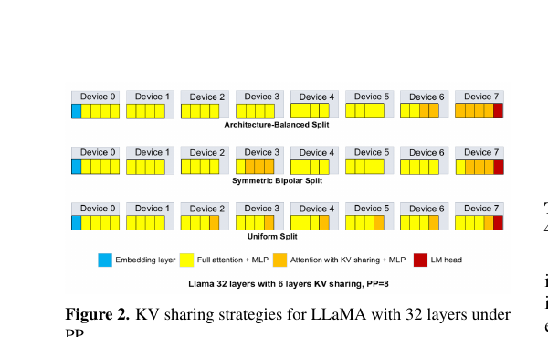
• Uniform: spread the $m$ KV-sharing conversions roughly evenly across stages, starting from the last stage and moving left. Rationale: reduce total FLOPs broadly without assuming where the bottleneck is.
• Symmetric Bipolar: allocate conversions from two anchor points — the last stage and the middle stage — moving left symmetrically from each. Rationale: useful if imbalance isn’t localized purely at the tail (e.g., if the middle of the network also happens to be unusually expensive for some architectural reason).
• Architecture-Balanced: allocate conversions preferentially to whichever stage is currently the bottleneck (typically the tail stage, because of the LM head), greedily reducing $\max_i F_{\text{stage}_i}$ directly.

Design choice, with alternative and boundary. Why should Architecture-Balanced win, and when might it not? The why-it-works argument is straightforward: since the objective (Eq. 4) is literally defined by the single worst stage, any FLOPs reduction that doesn’t land on that stage is wasted from FIR’s perspective — it lowers total model FLOPs (which is a real cost, and matters for pure compute/FLOPs-per-dollar reasoning) but does nothing for pipeline throughput, because the pipeline still waits on the same slow stage. Uniform and Symmetric Bipolar both spend part of their budget on stages that may not be on the critical path, which is provably (by construction) a less efficient use of the same conversion budget for this specific objective. The obvious alternative — Uniform placement — is exactly the kind of “spread it around, be fair” heuristic that seems reasonable if you don’t have FIR’s specific insight that only the max matters; it would be the natural first guess for someone who hadn’t thought carefully about which stage actually gates pipeline throughput. The boundary condition where Architecture-Balanced could underperform: if the imbalance isn’t concentrated in one place but is genuinely spread across multiple stages roughly equally (e.g., a hybrid architecture where cost heterogeneity is diffuse rather than localized to one bottleneck), then greedily emptying the single current-max stage risks the “over-correction” failure mode discussed in Section 5.2 below — shifting the bottleneck elsewhere rather than eliminating it — and Symmetric Bipolar’s more distributed strategy might actually be more robust in that regime, though the paper doesn’t test this scenario directly since LLaMA2’s architecture happens to concentrate its imbalance almost entirely at the tail (the LM head).

Table 1 (paper’s Table 2) confirms the intuition quantitatively for LLaMA2-7B, PP=8, with $m=4$ KV-sharing conversions:

PP split strategy	FLOP Imbalance Ratio
Baseline (no conversion)	1.1195
Uniform	1.1038
Symmetric Bipolar	1.0683
Architecture-Balanced	1.0004

Architecture-Balanced gets within 0.04% of perfect balance with the same conversion budget that leaves Uniform at 10.4% excess — a roughly 260x reduction in residual imbalance for the identical amount of “spend.”

4.3 Algorithm 1: tail-first, bottleneck-tracking greedy conversion

Figure 4 below sketches the two-stage architecture of the whole procedure — an offline planning pass that runs once per PP configuration, feeding a training/inference job that never has to know KV-Pipe ran at all (the converted checkpoint just looks like an ordinary, slightly cheaper model):

flowchart TD
    subgraph offline["Offline, one-time pre-processing"]
        A["PP partition {S_i} + per-layer FLOPs F_l(0), F_l(1)"] --> B["Compute baseline stage FLOPs & FIR (Eq. 4-5)"]
        B --> C{"FIR <= 1+eps?"}
        C -- no --> D["Target stage i* = tail, or current argmax if tail already OK"]
        D --> E["Convert deepest unconverted layer in stage i*"]
        E --> F["Update stage FLOPs, recompute FIR"]
        F --> C
        C -- yes --> G["Conversion mask z finalized"]
    end
    subgraph deploy["Deployed checkpoint"]
        G --> H["Training: balanced PP stages, higher MFU"]
        G --> I["Inference: smaller KV cache, faster long-context decode"]
    end

Figure 4 (structural summary of Algorithm 1): a one-time offline loop produces a single conversion mask that pays off twice — once during training as stage balance, once during inference as cache compression. This two-benefit structure, from one artifact, is the paper’s central practical selling point.

Here is the full procedure, given as numbered pseudocode (paper’s Algorithm 1), followed by a step-by-step prose walkthrough.

Algorithm 1: KV-Pipe (Architecture-Balanced)
Require: PP partition {S_i}_{i=1}^{P} with ordered layers in each stage;
         full-attn and KV-share FLOPs {F_l(0), F_l(1)} for l = 1..L;
         LM-head FLOPs F_LM-Head; tolerance epsilon > 0;
         max conversions m (default m = L).
Ensure:  Conversion mask z in {0,1}^L; updated stage FLOPs {F_stage_i};
         achieved FIR.

 1: z <- 0                                          // start with no conversions
 2: for i = 1 to P:
 3:     F_stage_i <- sum_{l in S_i} F_l(0) + [i == P] * F_LM-Head
 4: Compute FIR using Eqs. (4)-(5)
 5: t <- 0
 6: i <- P                                          // start from the last stage
 7: while FIR > 1 + epsilon and t < m:
 8:     i_star <- i
 9:     if F_stage_{i_star} <= (1 + epsilon) * F_avg:
10:         i_star <- argmax_j F_stage_j             // tail no longer bottleneck; retarget
11:     end if
12:     l_star <- max{ l in S_{i_star} : z_l == 0 }  // deepest unconverted layer in stage i_star
13:     if l_star is undefined:
14:         break                                     // no convertible layers remain here
15:     end if
16:     z_{l_star} <- 1                               // convert this layer
17:     delta_F <- F_{l_star}(0) - F_{l_star}(1)       // FLOPs saved, > 0 by construction
18:     F_stage_{i_star} <- F_stage_{i_star} - delta_F
19:     t <- t + 1
20:     recompute F_avg (Eq. 5) and FIR (Eq. 4)
21: end while
22: return z, {F_stage_i}, FIR

Prose walkthrough, line by line. The algorithm initializes with zero conversions and computes the baseline stage FLOPs and FIR (lines 1–4) — this is just the “before” snapshot from Section 3. It then enters a loop that starts pointed at the last stage (line 6), since architecturally the last stage is the typical bottleneck (LM head). On each iteration, it first checks whether the currently-targeted stage is still the bottleneck (line 9): if the tail stage has already been brought down to within tolerance $\epsilon$ of the average, the algorithm explicitly retargets to whatever stage is now the actual maximum (line 10) — this is the “bottleneck-tracking” behavior that distinguishes KV-Pipe from a naive “always convert the tail” heuristic, and it’s what allows the algorithm to keep making progress even after the original bottleneck has been neutralized.

Within the selected stage, the algorithm picks the deepest remaining full-attention layer (line 12) — i.e., converts layers “last-layer-first” within a stage. It converts that one layer (line 16), computes exactly how much FLOPs that conversion saved (line 17, guaranteed positive since KV-sharing is strictly cheaper than full attention), applies the update to that stage’s running FLOPs total (line 18), and recomputes the global FIR (line 20) to check the stopping condition again. The loop terminates under any of three conditions: FIR has reached the tolerance band ($\le 1+\epsilon$), the conversion budget $m$ has been exhausted, or there are no more convertible (unconverted, full-attention) layers left in the currently-targeted stage (line 13–14, a safety break to avoid an infinite loop if a stage runs out of layers to sacrifice).

Why last-layer-first within a stage? The paper doesn’t derive this from first principles, but the implicit reasoning (confirmed empirically in Section 5.4’s quality-preservation results) is a bias toward converting deeper layers in the network before shallower ones, on the general intuition — widely observed in layer-pruning and layer-skipping literature — that later layers in a Transformer tend to be more redundant / less critical to output quality than earlier layers, which build up more fundamental representations. Combined with “last stage first” (targeting the bottleneck stage, which for a tail-heavy architecture is also the last stage in the network), this compounds into a policy that happens to concentrate conversions in the network’s final quarter — which Section 5.4 shows empirically preserves validation perplexity almost exactly.

Runtime cost. The paper is explicit that this is a cheap, offline, one-time procedure: it requires only the PP partition (already fixed by your parallelism configuration) and a lightweight per-layer FLOPs estimate (either analytically derived or from a single profiling pass — not from running full training). Each iteration of the loop does constant-time work (updating one stage’s running total, comparing $P$ stage totals to find the current max) — with $P \le 16$ in practice and $m$ typically a small handful of layers, the total algorithm runtime is negligible compared to any actual training or serving run it precedes.

5. Experiments and results, unpacked

5.1 Setup

The paper evaluates LLaMA2-7B (32 layers) as the primary case-study model, with pipeline degree $P \in \{2, 4, 8\}$ and sequence lengths $S \in \{4K, 8K\}$, holding tensor-parallel and context-parallel degrees fixed to isolate pure PP effects. The main results run on 8× Huawei Ascend 910B NPUs using MindSpeed-LM’s 1F1B schedule (no interleaving); a second, independent set of experiments on 8× NVIDIA V100 GPUs validates that the trends generalize across hardware backends and across four different model families (LLaMA2-7B/13B, LLaMA3-8B, Qwen2.5-14B). The evaluation metric is Model FLOPs Utilization (MFU), defined as

$$\mathrm{MFU} = \frac{F_{\text{model}} \cdot \mathrm{Throughput}}{F_{\text{peak}}}, \tag{8}$$

where $F_{\text{model}}$ is FLOPs-per-iteration, Throughput is measured iterations/second, and $F_{\text{peak}}$ is the device’s peak FLOPs/second scaled by device count — the standard measure of how close a training run gets to the hardware’s theoretical compute ceiling.

5.2 Headline NPU result: MFU gains that grow with pipeline depth

Table 2 (paper’s Table 3) reports the NPU best-result summary — baseline 1F1B (no KV sharing) versus the best KV-Pipe configuration (Architecture-Balanced at its MFU-optimal budget) for each of three settings:

Config	MFU (baseline→KV-Pipe)	Relative MFU gain	Iteration time change	FIR (baseline→KV-Pipe)
S=4K, PP=2, SKV=8	62.45%→64.39%	+3.10%	-4.90%	1.0182→1.0101
S=8K, PP=4, SKV=6	61.28%→63.93%	+4.32%	-7.56%	1.051→1.018
S=8K, PP=8, SKV=4	56.32%→61.49%	+9.17%	-9.80%	1.1194→1.0004

The pattern that jumps out is monotonic: gains grow with pipeline depth ($P$). Going from $P=2$ to $P=8$, the relative MFU improvement roughly triples (3.10%→9.17%). This is not a coincidental correlation — it follows directly from the definition of FIR and how bubbles scale. At low PP degree, there are fewer devices to keep synchronized, so even a moderately imbalanced stage only costs a small fraction of total pipeline time in bubbles. At high PP degree, more devices are waiting on the single bottleneck stage simultaneously, and — critically — the baseline FIR itself is worse at PP=8 (1.1194) than at PP=2 (1.0182) in this table, because splitting 32 layers into 8 stages of 4 layers each means the LM head’s fixed cost is a larger relative share of a single (smaller) stage’s total FLOPs than it would be in a bigger stage. Both effects compound: more devices are idle, and each one is idle for a proportionally larger fraction of total pipeline time.

5.3 The imbalance metric tracks utilization — and a non-monotonic surprise

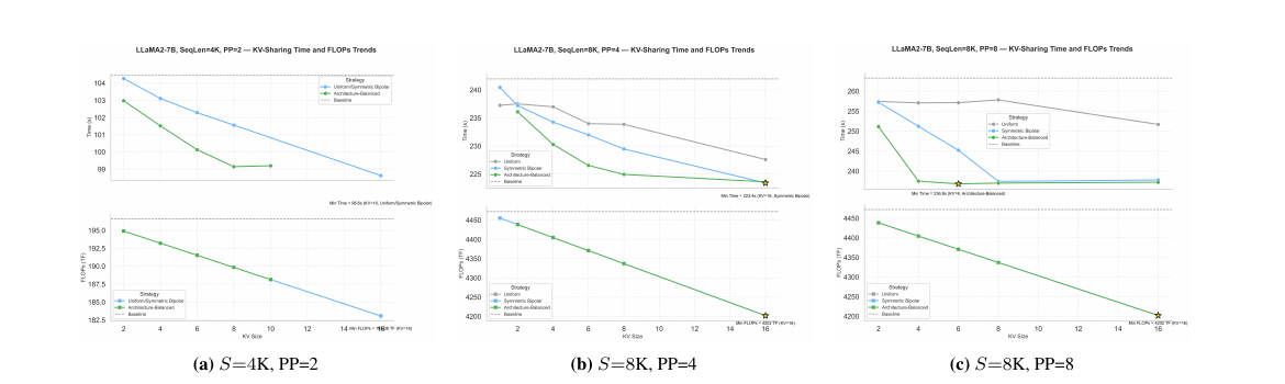
One of the paper’s more interesting empirical findings is that MFU is not monotonic in the KV-sharing budget. Sweeping the number of converted layers (Figure 2, paper Fig. 3) reveals that MFU rises sharply as you convert the first few layers, peaks at an intermediate budget, and then declines if you keep converting more layers — even though total model FLOPs keeps decreasing monotonically the whole time (Figure 3, paper Fig. 4, bottom rows).

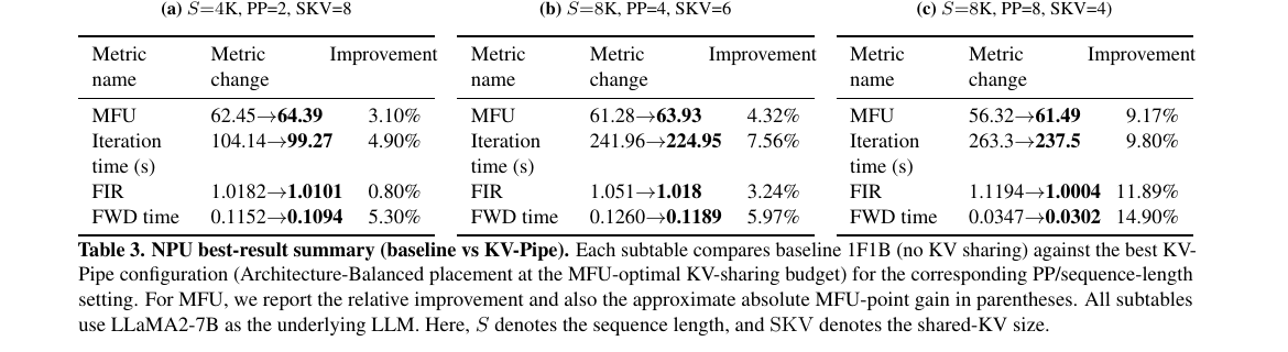
Why does more KV sharing eventually hurt MFU, if it keeps reducing total FLOPs? This is the paper’s central mechanistic insight, and it’s worth deriving carefully rather than just quoting. Recall FIR is defined relative to the current max-stage FLOPs, not total FLOPs. Early conversions (following Algorithm 1’s bottleneck-tracking logic) target the tail stage specifically, so they reduce $\max_i F_{\text{stage}_i}$ directly — this shrinks the numerator of FIR while barely touching the denominator (average FLOPs across all stages, which only drops by that one stage’s small contribution to the total), so FIR drops toward 1 quickly, bubble time shrinks, and MFU rises. But once the (originally-bottleneck) tail stage has been brought down to roughly the average, Algorithm 1’s retargeting logic (line 9-10 in the pseudocode) has no more “free” reductions to apply there — it must start converting layers in whatever stage is now the max, which by construction is a stage that started out not being the bottleneck. Every conversion beyond the original bottleneck’s “fair share” starts shifting the bottleneck to a different stage rather than eliminating it, which the paper calls “over-correction”: FIR starts rising again (even as total FLOPs keeps falling), reintroducing bubbles at the new critical stage, and MFU falls. This is exactly why the MFU-optimal shared-KV size in the NPU experiments (KV=8 at $P=2$, KV=6 at $P=4$, KV=4 at $P=8$) is an interior point of the sweep, never the largest tested budget — a clean empirical confirmation of the paper’s stated systems insight: for pipeline efficiency, the dominant objective is minimizing stage imbalance, not minimizing total FLOPs.

Table 3 (paper’s Figure 4 data, summarized) supports this from the time/FLOPs-sweep angle directly:

Iteration time and FLOPs sweeps confirm that the time-minimizing budget doesn’t always coincide with the MFU-maximizing budget either, because MFU is specifically sensitive to bubble overhead caused by imbalance, while raw iteration time is affected by total compute reduction as well.

5.4 The quality–efficiency trade-off: does converting layers hurt the model?

Cross-layer KV sharing permanently changes model architecture — it’s not a free lunch in the sense of “same model, faster execution”; it’s “a slightly different, cheaper model.” So the paper runs a dedicated evaluation of validation perplexity and downstream task accuracy (average over MMLU, HellaSwag, ARC-Challenge, TruthfulQA) for the exact KV-Pipe configurations selected by the algorithm, comparing against full-attention baselines and a fixed “Echo-style” heuristic that always converts the last 25% of layers regardless of measured imbalance:

Setting	Method	SKV	Converted layers	Val. PPL ↓	Downstream Avg. ↑	MFU / Iter. time change
S=4K, PP=2	Full-attn baseline	0	–	5.54	52.2	0.00% / 0.00%
S=4K, PP=2	Echo-style 25%	8	25–32	5.51	51.9	+2.85% / -4.35%
S=4K, PP=2	KV-Pipe, optimal	8	25–32	5.51	51.9	+3.10% / -4.90%
S=8K, PP=4	Full-attn baseline	0	–	5.67	52.5	0.00% / 0.00%
S=8K, PP=4	Echo-style 25%	8	25–32	5.50	52.0	+3.70% / -6.35%
S=8K, PP=4	KV-Pipe, optimal	6	27–32	5.50	52.0	+4.32% / -7.56%
S=8K, PP=8	Full-attn baseline	0	–	5.47	52.2	0.00% / 0.00%
S=8K, PP=8	Echo-style 25%	8	25–32	5.53	52.0	+6.80% / -8.10%
S=8K, PP=8	KV-Pipe, optimal	4	29–32	5.49	52.2	+9.17% / -9.80%

The most quality-conscious finding is at PP=8: KV-Pipe uses fewer KV-sharing layers (4 vs. 8) than the fixed Echo-style heuristic, yet achieves both better validation perplexity (5.49 vs. 5.53) and better downstream accuracy (52.2 vs. 52.0), while also delivering more MFU improvement (9.17% vs. 6.80%). This is a genuinely nice result to see spelled out explicitly: KV-Pipe’s adaptive, imbalance-driven budget selection isn’t just a system-efficiency win — because it converts fewer layers than a fixed 25%-of-network heuristic while achieving a larger speedup, it’s simultaneously a quality win. The paper’s honest framing (see design-choice discussion below) is that the practical advantage here is a better quality–sharing-budget–efficiency operating point, not a universal claim that “less sharing is always better than more” — at PP=2, the fixed 25% rule and KV-Pipe happen to select the identical layer set (25–32), because the imbalance there already requires most of that budget to correct.

Design choice: why does KV-Pipe’s adaptive budget beat a fixed 25% rule? The mechanism is exactly the over-correction story from Section 5.3: the fixed Echo-style baseline always converts 8 layers regardless of how much correction is actually needed, so at PP=8 (where only 4 conversions are needed to reach FIR≈1), it converts 4 more layers than necessary — layers 25–28, which Table 4’s data implies fall earlier in the “second half” of the network than KV-Pipe’s chosen 29–32, and by the paper’s own late-layers-are-more-redundant intuition, are presumably somewhat more consequential for the model’s function. Those 4 extra conversions cost some quality (5.53 vs 5.49 PPL) for no additional systems benefit (Echo-style’s over-corrected imbalance actually reduces the achieved MFU gain, as discussed above) — a lose-lose relative to stopping earlier once FIR is already near 1. The obvious alternative to KV-Pipe’s adaptive stopping — “just convert a fixed fraction and move on” — is simpler to implement but has no principled way of knowing when to stop, which this table shows can cost you on both axes simultaneously.

Boundary condition, stated by the paper explicitly (an admirable design decision): the “later layers are safer to convert” pattern observed here is an empirical regularity for this specific model family and these specific configurations — the paper’s Appendix A.3 adds an explicit “Optional Safe-Layer Guardrail” mechanism (a user-settable minimum normalized depth $\alpha$ below which conversion is disallowed, Eq. 9–10 in the appendix) precisely because the authors do not want to claim, as a theoretical guarantee, that early-layer conversion is universally safe or that the bottleneck can never move to an earlier stage in some other model or PP layout. This is exactly the kind of design-choice honesty that should be more common in systems papers — building in a guardrail for the case where your own empirical pattern doesn’t generalize, rather than silently assuming it always will.

5.5 Sensitivity ablations: placement policy, stopping tolerance, and imbalance signal

Table 4 (paper’s Table 9) runs three separate sensitivity studies, all on LLaMA2-7B at PP=8, S=8K:

Ablation	SKV	Converted layers	Val. PPL ↓	Downstream Avg. ↑	MFU / Iter. time change
Uniform placement	4	17, 22, 27, 32	5.50	52.1	+6.40% / -7.00%
Symmetric bipolar	4	17, 18, 31, 32	5.50	52.1	+7.10% / -7.60%
Architecture-Balanced	4	29–32	5.49	52.2	+9.17% / -9.80%
$\epsilon=0.02$	5	28–32	5.50	52.1	+9.05% / -9.65%
$\epsilon=0.05$ (default)	4	29–32	5.49	52.2	+9.17% / -9.80%
$\epsilon=0.10$	3	30–32	5.48	52.2	+8.60% / -9.20%
FIR-guided	4	29–32	5.49	52.2	+9.17% / -9.80%
Max-stage-time guided	4	28–31	5.49	52.2	+8.90% / -9.45%

Three separate takeaways: (1) at a matched SKV=4 budget, Architecture-Balanced clearly dominates Uniform and Symmetric Bipolar, confirming Section 4.2’s argument that placement location matters more than raw conversion count. (2) The stopping tolerance $\epsilon$ is not a sensitive hyperparameter over the tested range — moving from $\epsilon=0.02$ to $\epsilon=0.10$ only shifts the selected budget from 5 to 3 layers and MFU gain from 9.05% to 8.60%, meaning the method doesn’t require careful tuning to get most of the benefit. (3) FIR (the cheap analytic proxy) versus direct measured max-stage-time as the imbalance signal give nearly identical results (9.17% vs. 8.90% MFU gain) — a useful finding because FIR requires only static FLOPs estimates, while measured stage-time requires an actual profiling run; the paper frames this appropriately as “FIR is a useful low-cost signal for this workload,” not “FIR is provably as good as measured timing in general,” since FLOPs and wall-clock time can diverge whenever a stage is memory-bound or communication-bound rather than compute-bound.

5.6 Composability with a stronger pipeline scheduler (Seq1F1B)

A natural worry about any pipeline-balancing technique is whether it’s actually just re-deriving a benefit that a better scheduler would already capture — i.e., is KV-Pipe redundant with existing bubble-reduction work? The paper tests this directly by layering KV-Pipe on top of Seq1F1B (a stronger, sequence-level pipeline schedule that reduces bubbles through more fine-grained scheduling, evaluated on GPUs since the Ascend software stack didn’t support it at experiment time — an implementation limitation the paper flags honestly rather than silently working around):

Model / Setting	Method	MFU	Iter. time
LLaMA2-7B, PP=8, 8K	1F1B	39.0%	305s
LLaMA2-7B, PP=8, 8K	Seq1F1B	47.0%	265s
LLaMA2-7B, PP=8, 8K	Seq1F1B + KV-Pipe	50.0%	248s
LLaMA2-13B, PP=8, 16K	1F1B	39.5%	960s
LLaMA2-13B, PP=8, 16K	Seq1F1B	48.5%	820s
LLaMA2-13B, PP=8, 16K	Seq1F1B + KV-Pipe	52.0%	750s

Adding KV-Pipe on top of Seq1F1B yields a further MFU gain of roughly 6.4% (LLaMA2-7B) and 7.2% (LLaMA2-13B) relative to Seq1F1B alone — direct evidence that scheduling-level bubble mitigation (Seq1F1B’s contribution) and stage-workload balancing (KV-Pipe’s contribution) address genuinely different sources of inefficiency and stack additively rather than being redundant with each other. This is a meaningful result because it rules out the simplest possible objection to the whole paper: that KV-Pipe’s gains would simply evaporate under a better scheduler.

5.7 Cross-hardware and cross-model generalization (8×V100 GPUs)

To check that the NPU results aren’t an artifact of a specific hardware/software stack, the paper re-runs the full PP-focused evaluation on 8×NVIDIA V100 GPUs across four model families (LLaMA2-7B, LLaMA2-13B, LLaMA3-8B, Qwen2.5-14B), three PP degrees, and three context lengths, comparing 1F1B, Seq1F1B, and KV-Pipe:

The pattern from the NPU experiments replicates cleanly: KV-Pipe consistently beats both 1F1B and Seq1F1B across every one of the 36 combinations shown, and the margin of improvement grows both with pipeline depth (largest at PP=8) and with context length (largest at S=16K) — for example, LLaMA2-13B at S=16K, PP=8 goes from 39.5% MFU (1F1B) to 52.0% MFU (KV-Pipe), a 960s→750s iteration-time reduction. The context-length trend makes sense mechanistically: at longer sequences, attention’s quadratic-in-sequence-length cost becomes a larger fraction of total layer FLOPs, so converting attention layers to KV-sharing removes a proportionally larger chunk of compute, giving KV-Pipe more room to rebalance.

5.8 The inference-side “double benefit”: same conversion, different payoff

Because the layers converted for training-time pipeline balancing are the same layers that classical KV-sharing work uses for inference-time cache compression, KV-Pipe’s converted checkpoint gets an inference-time speedup “for free” — no separate mechanism needed. The paper demonstrates this with a dedicated inference case study on LLaMA2-7B under standard multi-head attention (MHA, i.e. no grouped-query sharing already baked in), measuring end-to-end decoding throughput at long context lengths with 50% of layers converted to KV sharing:

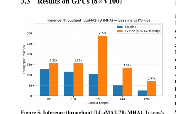
The throughput improvement grows sharply with context length: 1.22x at 8K tokens, climbing to 1.35x at 16K, 2.72x at 32K, 2.57x at 64K, and 2.77x at 128K. This is exactly what you’d expect from the mechanism: at short contexts, KV-cache size and redundant projection work are a small fraction of total decode cost, so removing some of it barely moves the needle; at long contexts, KV-cache memory pressure and attention cost dominate decode time, so the same relative reduction in KV-cache growth and projection work translates into a much larger relative throughput gain. (The dip in relative speedup from 32K to 64K, before it rises again at 128K, is not discussed in the paper’s main text — plausibly a batch-size or memory-pressure crossover effect specific to the measured hardware configuration, but this is speculation on the reviewer’s part, not something the paper explains.)

An appendix extension (Table 13, referenced but not reproduced numerically here since the paper text was partially compressed in the available extraction) confirms the same benefit persists under grouped-query attention (GQA) — a more deployment-realistic setting where $K$/$V$ projections are already reduced relative to MHA — with reported throughput gains of approximately 7.3% on LLaMA3-8B and 8.2% on Qwen2.5-14B. The gains are smaller under GQA than under MHA, which makes sense: GQA has already captured some of the K/V-reduction benefit that KV-sharing would otherwise provide, so there’s proportionally less headroom left for KV-Pipe’s conversion to remove.

5.9 Comparison against prior pipeline-partitioning systems

To directly benchmark against dedicated pipeline-partitioning research (not just scheduling variants), the paper reproduces the DawnPiper/vPipe evaluation setting (8×NVIDIA A100 40GB GPUs, 8 pipeline stages) and layers KV-Pipe’s rebalancing on top of the strongest baseline:

Model	Method	Pipeline mode	Max batch	Avg. speed (samples/s)	Speedup vs. vPipe-AS	Stage imbalance $\max_i t_i / \text{avg}_i t_i$
GPT-2 770M	GPipe	Sync.	7	16.0	0.56x	1.06
GPT-2 770M	vPipe-AS	Async.	16	28.7	1.00x	1.05
GPT-2 770M	DawnPiper-AS	Async.	20	33.0	1.15x	1.03
GPT-2 770M	KV-Pipe	Async. + SKV rebalance	20	34.5	1.20x	1.02
T5 780M	GPipe	Sync.	80	56.0	0.48x	1.42
T5 780M	vPipe-AS	Async.	180	116.0	1.00x	1.25
T5 780M	DawnPiper-AS	Async.	220	155.0	1.34x	1.12
T5 780M	KV-Pipe	Async. + SKV rebalance	220	163.0	1.41x	1.07

KV-Pipe improves average throughput over DawnPiper-AS by roughly 4.5% (GPT-2) and 5.2% (T5), while reducing the measured stage-imbalance ratio from 1.03→1.02 and 1.12→1.07 respectively. The paper is careful to frame this correctly: “these results should be interpreted as evidence that changing the per-layer cost profile can provide additional headroom beyond partition search, not as a claim that KV-Pipe subsumes general PP partitioning methods.” DawnPiper and vPipe search over where to place layers; KV-Pipe changes how expensive the layers are — the two are naturally complementary rather than competing solutions to the same problem, since a partition search can, in principle, be run on top of a model whose per-layer costs have already been reshaped by KV-Pipe.

6. Limitations

The paper is unusually forthright about scope limits, and it’s worth restating them plainly rather than glossing over them:

• Quality validation is limited to LLaMA2-7B. Perplexity and downstream-accuracy validation (Section 5.4) is conducted only on LLaMA2-7B. The LLaMA2-13B, LLaMA3-8B, and Qwen2.5-14B experiments provide systems-level efficiency evidence only — throughput and MFU numbers — and the paper explicitly states these are not used to claim architecture-independent quality preservation.
• No coverage of MoE or hybrid architectures. The paper does not assume its dense-LLaMA-family observations (e.g., “later layers are safer to convert”) transfer to Mixture-of-Experts models, Transformer–SSM hybrids (Mamba/Jamba-style), or other training regimes with fundamentally different per-layer cost structure.
• PP degree capped at 8. All experiments use $P \le 8$. The paper flags $P \in \{16, 32\}$ and very large models as open future work, noting that at larger scale the relative contribution of the LM head and the location of the critical stage may shift, which could change how the bottleneck-retargeting logic behaves in practice.
• Greedy, not globally optimal. Algorithm 1 is explicitly a lightweight offline heuristic. The paper does not claim it finds the globally optimal layer-conversion assignment among all $\binom{L}{\le m}$ possibilities — only that it’s a fast, interpretable, empirically effective approximation for the tested settings.
• Hardware coverage gap for the Seq1F1B composability experiment. Seq1F1B requires scheduler-level runtime support that the paper’s Ascend 910B software stack didn’t have at experiment time, so that specific composability result is GPU-only — an implementation gap, not a claim about KV-Pipe itself, but still a gap in cross-hardware coverage for that one experiment.
• No joint optimization of PP placement + KV-sharing placement + a quality constraint. The paper explicitly names this as an interesting open direction rather than something it attempts.

7. Critical analysis

(a) Weaknesses and flaws specific to this paper. First, the “Architecture-Balanced beats Uniform and Symmetric Bipolar” result (Section 4.2, Table 1) is measured on exactly the architecture where the imbalance is maximally concentrated in a single, predictable location — the tail stage carrying the LM head. This is close to a best-case scenario for a greedy, bottleneck-targeting strategy. The paper never tests a case where imbalance is genuinely diffuse — say, a hybrid model where cost heterogeneity is spread unevenly but not concentrated in one stage — which is precisely the scenario where Symmetric Bipolar’s more distributed budget allocation might plausibly outperform Architecture-Balanced. Without that experiment, the claim that “Architecture-Balanced is the best placement strategy” is really “Architecture-Balanced is the best placement strategy when the bottleneck is tail-concentrated,” a narrower and less exciting claim than the paper’s framing suggests.

Second, the GQA appendix result (Section 5.8, Table 13 in the original paper) is asserted with two summary percentages (7.3% and 8.2% throughput gains) but the underlying methodology — what shared-KV budget was used, whether it was independently re-tuned for the GQA setting or just carried over from the MHA experiments — is thin relative to the depth given to the MHA case study. Given that GQA already reduces the KV-cache-per-token baseline that cross-layer sharing further compresses, the interaction between GQA’s group size and KV-Pipe’s optimal conversion budget seems like exactly the kind of design-choice question the paper’s careful treatment elsewhere would normally dig into, and doesn’t here.

Third, the non-monotonic MFU-vs-budget curve (Section 5.3) is explained mechanistically (over-correction shifting the bottleneck), but the paper never attempts to predict the optimal budget analytically — it’s found by sweeping. For a paper whose whole pitch is “a lightweight, offline, no-online-tuning procedure,” needing an empirical sweep across the budget dimension to find the true MFU optimum is a meaningful practical gap: Algorithm 1 as stated will happily convert layers until FIR reaches its tolerance band, but Table 2’s data shows that stopping exactly at $\mathrm{FIR}\approx1$ is not always precisely the MFU-maximizing point either (compare the $\epsilon$ sensitivity table, where $\epsilon=0.10$‘s 3-layer conversion achieves marginally better perplexity than the $\epsilon=0.05$ default’s 4-layer conversion, at only a slightly lower MFU gain) — so there’s a genuine open question of whether FIR-driven stopping and true MFU-optimal stopping are exactly the same point, or merely close.

(b) Limitations the authors understate or omit. The paper’s Section 5.4 quality evaluation reports validation perplexity and a 4-task downstream average, which is a reasonably standard but fairly shallow quality bar for claiming “quality preservation” of a permanently modified architecture — there’s no evaluation of long-context-specific capabilities (e.g., needle-in-a-haystack retrieval, long-document QA), which is precisely the regime where KV-Pipe’s inference-side benefit (Section 5.8) is most emphasized, and precisely the regime where cross-layer KV sharing’s information-loss cost (later layers relying on earlier layers’ potentially-stale key/value representations) would be expected to bite hardest, if it bites at all. Claiming both “large long-context inference speedups” and “quality preservation validated at 4K/8K sequence lengths” without directly testing quality at the long context lengths where the inference benefit is measured is an internal inconsistency in evaluation scope that the paper doesn’t flag.

The paper also doesn’t discuss what happens when KV-Pipe’s chosen layer-conversion mask needs to change — e.g., if the PP partition is later re-tuned, or the model is fine-tuned for a different downstream task with different sequence-length distributions. Since conversion is a training-time architectural decision baked into the checkpoint, any mismatch between the FLOPs profile used to compute FIR (from a pretraining-time profiling pass) and the FLOPs profile the model actually experiences under a different downstream workload could silently degrade the balancing benefit without anyone noticing, since there’s no described mechanism for detecting or correcting this drift after deployment.

(c) Concrete, specific improvement suggestions. (1) Add at least one experiment on a genuinely non-tail-concentrated imbalance pattern — e.g., a synthetic hybrid Transformer-Mamba-style stage-cost profile, or an MoE model with per-layer token-routing variability — to test whether Architecture-Balanced’s dominance over Symmetric Bipolar and Uniform (Section 4.2) holds outside the LM-head-dominates-the-tail regime, or whether the paper’s own Symmetric Bipolar strategy would actually be preferable there. (2) Extend the quality evaluation (Table on Section 5.4) to include at least one long-context-specific benchmark (e.g., a passkey/needle retrieval test at 8K–32K context) run on the actual KV-Pipe-converted checkpoints used for the Section 5.8 inference throughput measurements, to close the evaluation-scope gap noted above. (3) Provide a lightweight closed-form or lookup-table approximation for the MFU-optimal conversion budget (even a rough heuristic derived from the FIR-vs-budget curve shape) so that practitioners don’t need to run the full empirical sweep from Figure 3 for every new model/PP configuration — this would meaningfully strengthen the “cheap offline pre-processing step” pitch by removing the one step (the budget sweep) that currently isn’t cheap or offline in the same sense as the rest of the pipeline.

8. Reproducibility notes

The paper specifies enough detail to reproduce the methodology (FIR formula, Algorithm 1 pseudocode, the three placement strategies) precisely, and the model/hardware configurations are stated explicitly (LLaMA2-7B/13B, LLaMA3-8B, Qwen2.5-14B; Ascend 910B via MindSpeed-LM; V100 via an unnamed but presumably standard PP implementation; A100 via the DawnPiper/vPipe benchmark harness). No code or checkpoint release is mentioned in the excerpted text available for this review, and per-layer FLOPs estimation (used as the core input to FIR) depends on implementation-level choices (analytical formula vs. one-time profiling pass) that could introduce small numerical differences across re-implementations, though the paper notes these differences are unlikely to be consequential given the algorithm’s demonstrated robustness to the stopping-tolerance hyperparameter.

9. Conclusion

KV-Pipe’s core contribution is conceptually small but genuinely useful: it identifies that cross-layer KV sharing, previously siloed as an inference-time memory optimization, is exactly the right tool to reshape a pipeline-parallel training run’s per-stage FLOPs profile, because both problems ultimately reduce to the same quantity — per-layer compute cost. The FIR metric gives a clean, cheap, interpretable way to measure stage imbalance, and the tail-first, bottleneck-tracking greedy algorithm built on top of it delivers consistent, hardware- and model-family-general MFU gains (3–9%) that compose additively with existing pipeline schedulers, plus a “free” inference-time throughput bonus at long context lengths from the very same converted layers. The honest caveats — quality validation confined to one model family, no test of genuinely diffuse (non-tail-concentrated) imbalance, and an admittedly greedy rather than globally optimal search — keep the paper’s claims appropriately scoped, and the paper is better for stating them explicitly rather than letting a reader discover them independently.