CacheRoute: Why Your LLM Load Balancer Is Fighting Your KV Cache

Review date: 2026-08-22 Author: Zhongzhu Zhou Paper reviewed: CacheRoute: Planned Prefix-Affinity Routing for Large-Scale LLM Serving Paper authors: Huang Cheng (Meta) arXiv: 2608.19677 Venue/Status: Preprint (cs.DC), August 2026

1. The tension this paper is actually about

Every production LLM serving stack faces a load-balancing decision that looks trivial and is not: when a new request arrives, which of your $R$ model-server replicas should handle it? The textbook answer is “whichever one is least busy right now” — spread load evenly, keep tail latency down. That answer is correct for stateless request routing, and it is wrong for LLM serving, because LLM inference engines are not actually stateless. Modern serving engines like vLLM and SGLang cache the key/value (KV) tensors computed during the prefix of a conversation, so that when the same prefix shows up again (a follow-up turn in a multi-turn chat, a repeated system prompt, a recurring retrieved context block), the engine can skip re-computing it — a strict latency and compute win called prefix caching.

The catch: that cached KV state lives on one specific machine. If a load balancer sprays successive requests for the same conversation across different replicas — which is exactly what “route to the least-loaded server” naturally does under any reasonable spreading policy — the cache on any single machine is essentially useless, because the next request for that same prefix probably won’t land there. You get low cache-hit rates and repeated prefill work, even though your fleet nominally has the memory capacity to cache everything.

The obvious fix is affinity: pin a given conversation (or business, or tenant) to one fixed destination so its cache reliably warms up and stays warm. But pure affinity has a mirror-image failure mode. If usage rates across conversations are skewed — and they always are, in any real deployment — pinning naively maps that skew directly onto server queues. The busiest conversation determines the busiest server’s queue, and that server’s tail latency becomes the fleet’s tail latency, no matter how idle the other 29 machines are.

So you are stuck between two failure modes that look opposite but share a root cause — neither policy is aware of both cache locality and load at the same time:

• Cache-blind balancing (e.g., power-of-two-choices): evens out load, destroys locality, throws away prefill work you already paid for.
• Naive fixed affinity (e.g., plain consistent hashing): preserves locality, but a single hot key can overload its pinned destination and dominate the fleet’s p99.

CacheRoute’s proposal is refreshingly unglamorous: don’t try to solve this reactively, request by request. Instead, periodically compute an offline routing plan from measured per-key request rates — a plan that jointly (a) decides which keys are “hot enough” to deserve a stable, cache-friendly assignment, and (b) places those assignments to balance expected load across destinations before a single request is dispatched. Sitting off the request path, the plan can afford exact accounting that a per-request router cannot.

What makes this paper worth a careful read is not that the individual techniques are novel — the paper is explicit that top-rate admission and longest-processing-time (LPT) list scheduling are textbook. What’s valuable is the measurement discipline: a large-scale (60-GPU, 70B-parameter) production-style evaluation, a second independent workload used specifically to test whether the first result generalizes, and — most unusually for a systems paper — an explicit, quantified account of the regimes where the technique loses to the naive baseline. Section 5.3’s honesty about two 32B workloads where affinity actively hurts capacity is the single most valuable contribution in the paper, and this review spends real time on it.

2. Prerequisites

2.1 What prefix caching actually buys you, and why it’s fragile

An autoregressive transformer decoder processes a prompt in two phases: prefill, where the entire input prompt is processed in parallel to produce the first output token (and, along the way, the KV tensors for every input token at every layer), and decode, where output tokens are generated one at a time, each attending back over all previously-computed KV tensors via the causal self-attention mechanism used throughout the Transformer architecture. Prefill cost scales with the square of the prompt length for the attention computation and linearly for the feed-forward layers; for prompts in the low thousands of tokens — realistic for a multi-turn chat with a system prompt and a growing history — prefill is a substantial, not-negligible chunk of total serving cost.

Prefix caching (introduced operationally by systems like vLLM’s PagedAttention and refined by SGLang’s RadixAttention) exploits an observation: if two requests share an identical token prefix, the KV tensors for that shared prefix are identical, because the transformer’s attention computation for token $i$ depends only on tokens $1, \dots, i$. So instead of recomputing the KV tensors for the shared prefix every time, the engine can cache them (typically as block-structured “pages” of KV state) and simply reuse them, computing fresh KV tensors only for the new suffix tokens. For a multi-turn conversation where each new turn appends to a stable history, this converts an $O(n^2)$-scaling prefill of the full context into an $O(n \cdot \Delta)$ prefill of only the new tokens $\Delta$ — a large practical win when $\Delta \ll n$.

The fragility: this cache is local to the machine that computed it. There is no free lunch that makes KV state magically available fleet-wide — cross-machine KV transfer is itself an active systems research area (see Mooncake and MemServe in the Related Work discussion below), and even where it exists, transferring gigabytes of KV tensors over the network is not free. The default assumption in most serving deployments is that if you want to reuse a prefix’s cache, the request carrying that prefix has to land back on the same machine that cached it. That’s the entire premise this paper is built on.

2.2 Why naive load balancing defeats prefix caching: a back-of-envelope argument

Consider a “business” (the paper’s term for a routing key — could equally be a tenant, a conversation thread, or an application) with steady request rate $\lambda_b$ requests/second, uniformly load-balanced across $R$ destinations by power-of-two-choices or similar. Because each request for this business is equally likely to land on any of the $R$ destinations (approximately, under a spreading policy), the mean time between two consecutive visits to the same destination scales as

$$T_{\text{revisit}} \approx \frac{R}{\lambda_b}. \tag{1}$$

This is a simple renewal-process argument: if requests arrive as a Poisson-like stream at rate $\lambda_b$ and are independently assigned to one of $R$ destinations with probability $1/R$ each, the sub-stream of requests landing on any particular destination is (approximately) Poisson with rate $\lambda_b / R$, so the expected gap between successive arrivals at that destination is $R/\lambda_b$.

The consequence is counter-intuitive and important: scaling up your fleet (increasing $R$) to handle more load actively makes prefix caching worse, because it lengthens the expected time before a given prefix’s cache entry gets revisited. If that revisit time exceeds the engine’s effective KV-cache eviction time (governed by memory pressure and the LRU-style eviction policy most engines use), the cache entry is gone before it’s ever reused, and every request pays full prefill cost regardless of how much aggregate cache capacity the fleet has. Figure 1 below visualizes exactly this relationship.

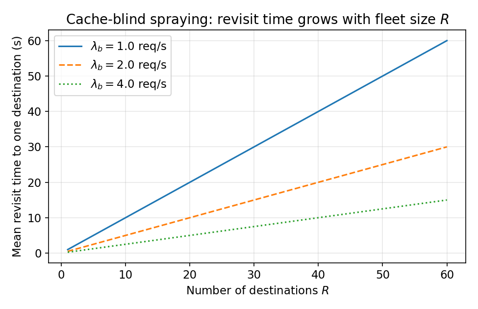
This is the paper’s Section 2.2 argument, and it’s the conceptual core that motivates everything else: a purely reactive, cache-blind balancer is structurally unable to preserve reuse at scale, no matter how sophisticated its load-balancing heuristic is, because the problem isn’t about picking the “best” destination per request — it’s about the statistics of how often any one destination gets revisited at all.

2.3 Longest-Processing-Time (LPT) scheduling — the classic algorithm CacheRoute repurposes

LPT list scheduling (Graham 1969) is one of the oldest results in scheduling theory. The setup: you have a set of jobs with known processing times, and $m$ identical machines; you want to assign jobs to machines to minimize the makespan (the time until the last machine finishes). The greedy LPT heuristic: sort jobs by decreasing size, and assign each job in turn to whichever machine currently has the least total assigned work. Graham’s classical result is a worst-case approximation bound: LPT’s makespan is never worse than $\frac{4}{3} - \frac{1}{3m}$ times the optimal makespan — a strong guarantee for an almost trivially simple algorithm.

CacheRoute repurposes this exact greedy rule, but the paper is careful to flag (Section 3.1, Table caption context) that Graham’s approximation bound does not apply verbatim to CacheRoute’s setting, because CacheRoute’s “jobs” are not atomic: a single hot key can be split across multiple destinations (replication), and the assignment carries a “distinct-destination” constraint (a key’s replicas must go to different machines). This is an honest and easy-to-miss caveat — many systems papers borrow a classical algorithm’s name and implicitly its guarantee; this one explicitly disclaims the guarantee while keeping the mechanism, which is the intellectually correct thing to do when you can’t verify the proof transfers.

3. Method: how CacheRoute actually builds a routing table

3.1 The planning objective

CacheRoute’s job is to build a table $T: b \mapsto \{$destinations$\}$ that maps each business key $b$ to one or more of the $R$ available destinations, recomputed periodically (once per “control interval,” not per request). The construction has three steps, and this review unpacks each one in turn with the exact algebra, then gives the full pseudocode.

Step 1 — load-based assignment count. For a business with measured rate $\lambda_b$, and a calibrated per-destination capacity ceiling $q_{\text{cap}}$ (derived empirically from a single destination’s latency/load knee — i.e., the QPS at which that one machine’s tail latency starts to blow up), the number of destinations $k_b$ that key $b$ should be replicated across is:

$$k_b = \max\left(1, \left\lceil \frac{\lambda_b}{q_{\text{cap}}} \right\rceil\right). \tag{2}$$

The intuition here is direct capacity accounting: if $\lambda_b \le q_{\text{cap}}$, one destination is enough ($k_b = 1$) and the whole rate $\lambda_b$ lands on that single machine, no worse off than the machine’s own ceiling. If $\lambda_b$ is bigger than one machine can handle, $k_b$ grows just enough that splitting $\lambda_b$ evenly across $k_b$ machines brings each machine’s share back at or below $q_{\text{cap}}$. Note precisely what this equation is not: it is not an eviction-time model, and it makes no claim about whether the KV cache will actually still be resident when the next request for $b$ arrives — it is purely a load-control rule. The paper is explicit about this distinction (Section 3.1), and it matters, because it’s exactly the kind of distinction that a less careful paper would blur, implicitly suggesting a cache-residency guarantee the method doesn’t actually provide.

Step 2 — warm-set admission. Not every business key gets a stable slot; if you tried to give every one of 128,824 observed keys in the paper’s primary workload a dedicated warm slot, you’d exceed available cache capacity many times over. So the planner treats the fleet’s admission budget as $C = R \cdot W$ total “warm-prefix slots” (where $W$ is a per-destination slot budget, chosen based on measured cache capacity), sorts all keys by decreasing $\lambda_b$, and admits keys greedily from the top until the cumulative $\sum k_b$ would exceed $C$:

$$\text{admit } b \text{ while } \sum_{b' \preceq b} k_{b'} \le C, \tag{3}$$

where $b' \preceq b$ denotes “keys with rate at least as high as $b$‘s, processed so far in the sorted order.” This is exactly the greedy “top-rate admission” the paper’s contribution list refers to — conceptually identical to admitting items into a knapsack by value density, except here every unit has equal size (one warm slot) and only value (rate) varies, which is what makes a simple greedy sort by $\lambda_b$ optimal for this simplified admission sub-problem (though the paper is careful to call out — Section 3.1 — that this equal-slot assumption breaks down for workloads with heterogeneous per-key prefix sizes, a real limitation discussed further in Section 6 below).

Step 3 — LPT placement. For every admitted key $b$, the planner creates $k_b$ “jobs,” each carrying an expected load of $\lambda_b / k_b$ (i.e., splitting the key’s total rate evenly across its assigned destinations). It then runs exactly the LPT heuristic from Section 2.3: process admitted keys in decreasing-rate order, and for each key’s set of $k_b$ jobs, greedily assign them to the $k_b$ currently least-loaded eligible destinations (with the “distinct-destination” constraint — a key’s own replicas can’t double up on one machine), updating each chosen destination’s running load tally as you go. Destinations start with an initial “expected cold-tail load” baseline to account for the unadmitted traffic they’ll also absorb via fallback routing (Step 4).

Step 4 — dispatch. Once the table $T$ is fixed for the control interval, request-time routing is a cheap lookup: an admitted key’s request goes to the least-loaded member of its own fixed set $T(b)$ (a small, pre-computed candidate set, not a fleet-wide search); any unadmitted key falls back to ordinary cache-blind power-of-two-choices across the whole fleet.

Here is the full procedure as numbered pseudocode, matching the paper’s Algorithm 1 but with each line’s intent spelled out:

Algorithm: Periodic Routing-Table Construction
Input:  measured rates {λ_b} for all observed keys b
        number of destinations R
        per-destination capacity ceiling q_cap
        total warm-slot budget C = R · W

1.  for each key b:
2.      k_b ← max(1, ceil(λ_b / q_cap))        # Eq. 2: how many destinations b needs
3.  end for
4.  sort all keys by decreasing λ_b
5.  admitted ← {}; running_total ← 0
6.  for each key b in sorted order:
7.      if running_total + k_b ≤ C:
8.          admitted ← admitted ∪ {b}
9.          running_total ← running_total + k_b
10.     else:
11.         skip b (falls back to power-of-two-choices at dispatch time)
12.     end if
13. end for
14. initialize L[r] ← expected_cold_tail_load(r) for each destination r ∈ [1, R]
15. for each admitted key b, in decreasing λ_b order:
16.     T(b) ← the k_b destinations with the k_b smallest current L[r] values,
              subject to: all k_b destinations are distinct
17.     for each destination r in T(b):
18.         L[r] ← L[r] + λ_b / k_b            # charge the split load to r
19.     end for
20. end for
21. output T (fixed for this control interval); admitted keys route within T(b);
    unadmitted keys fall back to power-of-two-choices at dispatch time.

The paper reports the empirical construction cost of this whole procedure: 345 milliseconds at $R = 30$ destinations for 128,824 business keys, with an asymptotic complexity of $O(|B| \log |B| + \sum_b k_b \log R)$ — dominated by the initial sort and the per-key search for the least-loaded eligible destination (implementable with a small heap over $R$ destinations). Because this plan is computed offline, off the request-serving path, it can afford this cost even though it would be far too slow to redo per-request.

3.2 Design choice deep-dive: why “periodic and stable,” not “reactive and per-request”?

This is the single most consequential design decision in the paper, and it deserves the why/alternative/boundary treatment the depth requirement asks for.

Why it works: A per-request reactive router (like Preble or DualMap, discussed in Section 4 below) has to make a routing decision using only the information available at that instant — current cache state estimates, current queue lengths — and it has to make that decision fast enough to sit on the hot serving path. This forces reactive routers into local, greedy decisions that can’t account for the global rate distribution across all keys simultaneously. CacheRoute instead moves the hard combinatorial part (which keys deserve stable placement, and how to balance their combined expected load) off the request path entirely, where it can afford an $O(|B| \log |B|)$ sort and a principled LPT pass over the entire observed rate distribution at once. The serving-time cost then collapses to a table lookup plus a small local comparison — cheap enough to sit on the hot path without adding meaningful latency.

The obvious alternative: Recompute assignments continuously (or every request) based on live state, the way Preble and DualMap do. This is strictly more reactive to sudden shifts in the traffic pattern — a periodic plan can go stale between recomputation intervals. And indeed, that staleness is a real, measured cost (Section 5.4): a one-interval-stale plan loses up to 3.0 percentage points of KV hit rate and 858 ms of p99 latency in the worst observed transition during a simulated rate drift. So the “why” for periodic planning is not “reactive approaches are strictly worse” — it’s a bet that the benefit of globally coherent, off-path optimization outweighs the cost of being slightly stale between recomputations, provided the recomputation interval is short relative to how fast the underlying rate distribution actually shifts in practice.

Where it fails / the boundary: The paper is unusually forthcoming about this. Section 5.4’s rate-drift experiment shows that recomputing the LPT plan from scratch changes 94.5% of key-to-destination assignments even though only 1.1% of keys actually change their replication count $k_b$ — meaning the LPT placement step is quite sensitive to small perturbations in the input, producing near-total plan churn from a modest rate shift. Installing a freshly recomputed plan then causes a transient 13.6-percentage-point KV-hit drop during the “rewarming” period as previously-warm destinations lose their assignments and new ones cold-start. The paper’s own conclusion (explicitly stated, not left implicit) is that a deployment should hold onto a stale plan until the measured staleness penalty exceeds the rewarming penalty of installing a fresh one — and that they have not built a churn-aware replanner that would mitigate this (an honest, flagged gap, discussed further in Section 8 of this review).

4. What CacheRoute is measured against

The paper compares against five baseline routing policies, each representing a different point on the affinity-vs-balance spectrum, all reimplemented under one common harness for fairness (the paper is explicit that these are not literal reproductions of the original published systems, just behavior-matched reimplementations under matched hardware):

• Flat-LB — power-of-two-choices, the cache-blind baseline representing “just balance load, ignore the cache entirely.”
• Sticky — plain consistent hashing (Karger et al. 1997): pure affinity, no load awareness at all.
• CHWBL — consistent hashing with bounded loads (Mirrokni et al. 2018): affinity with an explicit overflow cap, so a too-hot key spills excess requests elsewhere.
• DualMap — a two-candidate cache-and-load-aware reactive policy (Yuan et al. 2026), representing recent “smart” reactive routing.
• Preble — a prefix-history-and-live-load-aware reactive policy (Srivatsa et al. 2024), representing the strongest reactive contender.

Figure 2 sketches the full pipeline, from measured telemetry through to per-request dispatch, tying the algorithm back to the architectural picture:

flowchart LR
    subgraph offline["Offline, periodic (every control interval)"]
        A["Aggregate telemetry:<br/>per-key rate λ_b"] --> B["Top-rate admission<br/>(Eq. 3, greedy knapsack)"]
        B --> C["Load sizing<br/>k_b = ceil(λ_b/q_cap)<br/>(Eq. 2)"]
        C --> D["LPT placement<br/>against total expected load"]
        D --> E["Stable table T: b → destination set"]
    end
    subgraph online["Online, per-request"]
        F["Request with key b"] --> G{"b admitted<br/>in T?"}
        G -- "yes" --> H["Least-loaded member<br/>of fixed T(b)"]
        G -- "no" --> I["Cold-tail traffic:<br/>power-of-two-choices<br/>over all destinations"]
        H --> J["Model destination<br/>(native prefix KV cache)"]
        I --> J
    end
    E -.->|"table lookup"| G

Figure 2 (paper Fig. 1, redrawn): the two-timescale architecture — a slow, globally-optimized offline plan feeding a fast, per-request dispatch decision. This separation of concerns (plan once, dispatch cheaply) is the structural idea that makes the rest of the paper’s measurements possible.

5. Experiments and results, unpacked

5.1 The flagship result: 70B on 60 H100 GPUs

The main evaluation serves Llama-3.3-70B in fp8 precision across 30 tensor-parallel-2 destinations (60 H100 GPUs total), replaying a semi-synthetic workload built to match a real multi-tenant conversational-assistant traffic pattern: 128,824 opaque business keys with a Gini coefficient of 0.756 (heavily skewed — about 4% of keys generate 47% of requests, yet no single key exceeds 0.3% of total traffic, ruling out simple “just pin the top-1 key” special-casing).

At the primary 3.5-second p99 SLO threshold, across five paired random seeds:

Policy	Served KV hit	SLO capacity @3.5s (QPS)	p99 @ 100 QPS
Flat-LB	64.1 ± 1.3%	42 ± 20	5.7 s
Sticky	87.3 ± 2.4%	30	8.5 s
CHWBL	75.6 ± 0.8%	64 ± 11	3.8 s
DualMap	88.7 ± 1.9%	58 ± 22	5.3 s
Preble	72.0 ± 0.7%	76 ± 11	3.8 s
CacheRoute	93.2 ± 0.5%	176 ± 11	1.8 s

CacheRoute reaches 2.3× the SLO capacity of the strongest baseline (Preble) and 4.2× that of the cache-blind Flat-LB baseline. Figure 3 visualizes the capacity comparison and Figure 4 the latency-at-common-load comparison (the paper’s Figure 2 panels a and b).

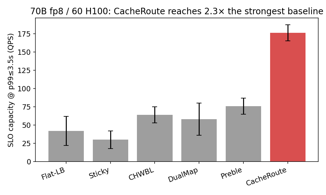
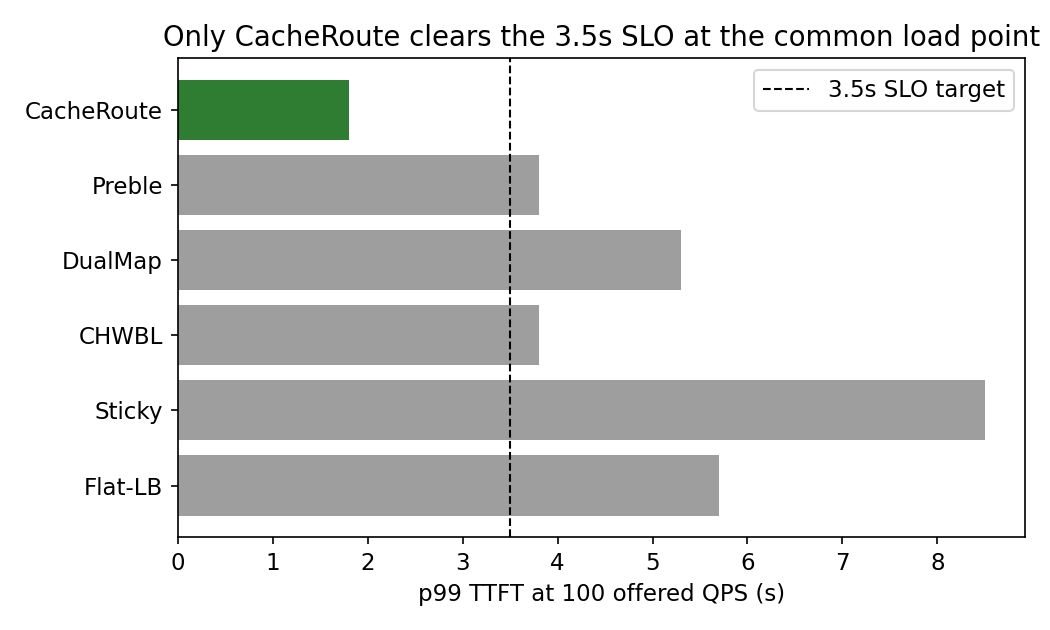
The mechanistic story behind these numbers, laid out carefully in Section 5.1, is worth stating precisely because it disambiguates why CacheRoute wins and not just that it wins: Sticky and DualMap both recover high cache-hit rates (87.3% and 88.7%, comparable to CacheRoute’s 93.2%) — so cache locality alone is not the differentiator. But their p99 latencies at 100 offered QPS are 8.5 s and 5.3 s respectively, far worse than CacheRoute’s 1.8 s, because their queue imbalance dominates the tail once load climbs. Conversely, Preble and CHWBL keep queues relatively even (p99 of 3.8 s each, decent) but their cache-hit rates fall to 72.0% and 75.6% — worse locality means more prefill work, which raises latency even with balanced queues. CacheRoute is the only policy in the comparison that achieves both high hit rate and low imbalance simultaneously, which is exactly what its joint admission-and-placement objective was designed to produce.

At a looser 5-second SLO the CacheRoute-over-Preble advantage narrows to 1.3× (180 vs 140 QPS); at a tight 2-second SLO, CacheRoute is the only policy to pass any tested load level at all — all five baselines are left-censored below the 30-QPS minimum tested. This SLO-dependence is itself informative: CacheRoute’s advantage is largest exactly where it matters most (tight, realistic production SLOs), and shrinks as the bar is lowered — a pattern that should make a reader trust the mechanism rather than suspect a cherry-picked operating point.

5.2 Generalization check: a second, independently-collected workload

Rather than stopping at one result, the paper repeats the experiment on an independently collected aggregate key-rate distribution on the same hardware. At a top-K128 active-set size (meaning only the top 128 keys by rate are actively driving load, roughly matching the primary workload’s effective admission footprint), the three cache-aware policies (CacheRoute, DualMap, CHWBL) all tie at 100 QPS — CacheRoute’s advantage doesn’t show up here. But expanding to a wider top-K256 active set separates them clearly: CacheRoute sustains 160 QPS versus 100 QPS for the best baseline (DualMap). The paper’s own framing of this is important and refreshingly precise: the comparison is useful precisely because it does not reproduce every cell of the first table — the advantage appears specifically once the active set outgrows the warm-slot allocation, i.e., once admission pressure actually starts to bind. This is a much more informative negative-and-positive result pairing than simply reporting “we replicated the win on a second dataset,” because it tells you the condition under which the win shows up rather than just asserting that it does.

5.3 Component ablation: disentangling affinity from placement

The most mechanistically illuminating experiment in the paper uses the smaller Llama-3.1-8B-Instruct testbed (30 single-H100 destinations) with synthetically injected “whale” keys — deliberately hot keys designed to stress-test the mechanism — to add CacheRoute’s components one at a time:

Configuration	KV hit	Load imbalance (max/mean)	SLO capacity
Flat-LB	56 ± 1.9%	1.00×	240
+ affinity (only)	88 ± 1.5%	3.46×	240
+ replication	88 ± 1.6%	2.60×	240
+ LPT (full CacheRoute)	90 ± 1.0%	1.24×	500 (ceiling)

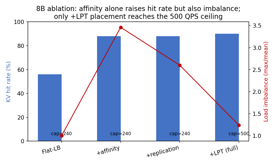
This table is the clearest evidence in the paper for the paper’s core thesis — that neither affinity nor balance alone is sufficient. Adding raw affinity nearly triples KV-hit rate (56% → 88%) but simultaneously blows up load imbalance to 3.46× — and crucially, capacity does not improve at all at this stage (still capped at 240 QPS), because the imbalance created by naive affinity is exactly canceling out the latency benefit of the higher hit rate. Adding load-proportional replication (splitting hot keys across multiple destinations) reduces imbalance somewhat (to 2.60×) but again capacity stays flat — replication without smart placement of the resulting sub-loads doesn’t help either. Only once LPT placement is added — actively balancing where those replicated sub-loads land — does imbalance drop to a manageable 1.24× and capacity jump all the way to the 500 QPS sweep ceiling (a right-censored result, meaning the true capacity might be even higher; the experiment simply didn’t push load far enough to find the actual knee). This ablation earns its place as the paper’s most important mechanistic evidence: it isolates that the combination of affinity and balanced placement is doing the work, not either ingredient alone.

5.4 The negative results: where affinity actively hurts

This is the section that most distinguishes this paper from typical systems-paper triumphalism, and it deserves to be read in full. Table 5 (below, redrawn as Figure 6) reports three “operating regimes”:

Regime	Flat-LB hit	Affinity hit	Capacity multiplier	Outcome
8B synthetic whales	9.3%	77.0%	2–6×	win
Aggregate A – 32B	1.1%	11.8%	0.50–0.67×	lose
Aggregate B – 32B	0.8%	8.5%	1.0×	tie

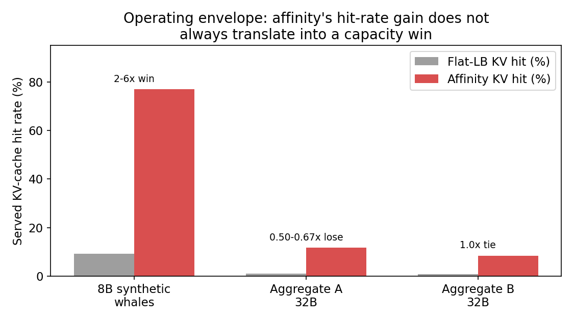
On two real-world-derived (de-identified, semi-synthetic) 32B aggregate workloads, enabling affinity moves the KV-hit rate only modestly (from roughly 1% to somewhere between 8.5% and 11.8%), and for Aggregate Workload A that modest hit-rate gain is not enough to outweigh the load skew that affinity introduces — capacity actually drops to 0.50–0.67× of the cache-blind baseline. This is exactly the failure mode the paper’s Section 2.2 argument predicts is possible when the “recoverable prefix work” available in a workload is small: if most requests don’t actually have a reusable prefix worth preserving (a low base hit rate even under perfect affinity), then affinity buys you almost nothing in cache terms while still concentrating load onto specific destinations, and you’re strictly worse off than just balancing.

The paper’s stated conclusion from this is unambiguous and, refreshingly, not softened: model size by itself does not distinguish these outcomes — both a 70B and a 32B model produced positive results in different workloads, and 32B alone also produced negative and tied results, so “affinity works better on bigger models” would be a wrong inference from this data, and the paper takes pains to preempt exactly that wrong inference.

5.5 Why the paper explicitly refuses to build an analytic residency predictor

Section 5.3 (labeled “Why we do not predict residency analytically” in the original) reports an experiment the authors ran and then chose not to build on: they tested a single-characteristic-time occupancy model (essentially, an attempt to analytically predict what fraction of requests would find their prefix still cached, based on rate and cache size) against the actual 70B fp8 engine, after carefully instrumenting the engine and passing seven separate isolation checks to confirm the instrumentation was trustworthy. The model still missed the actually-observed served hit rate by 14.3 percentage points at the median case and by a much larger 44.7 points at the 90th percentile — and the shape of the observed hit-rate curve (a sharp initial drop followed by a plateau) fell entirely outside the family of curves the tested analytic model could produce.

This is an unusually candid negative result to include, and it directly justifies the paper’s recommended deployment practice: use empirical shadow replay (run the candidate routing plan against real traffic without returning results to users, and measure the actual hit rate and latency) rather than trying to predict outcomes from a closed-form model. Reporting a negative modeling result that most papers would simply omit is a genuine strength of this work — it tells future practitioners not to waste time on an approach the authors already tried and found insufficient, and it’s honest about why it failed (curve shape mismatch) rather than just saying “it didn’t work.”

5.6 Burstiness and staleness sensitivity

Two further robustness checks round out the empirical section. First, replacing the smooth arrival process with a Gamma-distributed arrival process matched to the workload’s coefficient of variation (CV = 1.9, i.e., meaningfully bursty) reduces CacheRoute’s 3.5-second SLO capacity by exactly one ladder step, from 180 to 160 QPS, while Flat-LB stays pinned at 30 QPS regardless — showing the CacheRoute advantage survives realistic burstiness even if the absolute number degrades slightly. A separate check using a moving-block-bootstrap resampling of 22,639 real measured inter-arrival gaps (preserving short-range correlation structure that a pure Gamma process would miss) leaves CacheRoute essentially unaffected at 180 QPS / 93% hit rate, while Flat-LB becomes left-censored below its 30-QPS minimum — evidence that CacheRoute’s win isn’t an artifact of assuming unrealistically smooth arrivals.

Second, the rate-drift experiment discussed in Section 3.2 above (lognormal random walk perturbation of the primary rate vector over six control intervals, $\sigma = 0.3$) quantifies exactly how much a stale plan costs versus a freshly recomputed one, and how much a fresh installation itself costs in transient rewarming penalty — a genuinely useful operational finding for anyone deciding how often to recompute the plan in production.

6. Design choices, revisited with alternatives and boundaries

Equal-slot admission (treating every key’s warm-prefix footprint as the same size). Why it works: it keeps the admission sub-problem a simple greedy sort — no need to measure or estimate per-key prefix byte sizes, which would require additional instrumentation and complicate the math into a genuine knapsack problem (NP-hard in general, though well-approximated). The obvious alternative: a byte-aware admission scheme that weights each key by its actual reusable-prefix size divided by its rate (a value-density knapsack), potentially admitting more low-rate-but-tiny-prefix keys at the expense of high-rate-but-huge-prefix keys. Where it fails: the paper explicitly flags (Section 3.1 and again in Section 6) that this assumption “does not cover workloads with heterogeneous reusable-prefix sizes” — if your deployment has some tenants with 200-token system prompts and others with 20,000-token retrieved-document contexts, equal-slot admission will misallocate the warm-slot budget, likely over-admitting small-footprint keys relative to their actual value and under-admitting large ones, or vice versa depending on how $W$ was calibrated.

No KV cache migration or reservation (CacheRoute only changes where requests go, never touches cache contents). Why it works: it keeps CacheRoute fully decoupled from the serving engine’s internals — it works with whatever native eviction policy (typically LRU-like) the engine already implements, requiring zero engine modifications and making the technique broadly portable across vLLM, SGLang, or any other engine with prefix caching. The obvious alternative: actively migrate or pre-warm KV cache blocks to destinations before routing requests there (the approach taken by systems like Mooncake, discussed in Related Work), which could in principle eliminate cold starts entirely for newly-installed table entries. Where it fails: because CacheRoute doesn’t reserve cache space, an admitted key’s warm prefix can still be evicted by unrelated cold-tail traffic competing for the same cache — the paper explicitly notes this (Section 3.2) and it’s exactly why “served” hit rate (measured empirically) is used throughout rather than an assumed guarantee.

Fixed table for an entire control interval, rather than continuous adaptation. Already analyzed in depth in Section 3.2 above — the core tradeoff between global off-path optimization and staleness cost.

7. Limitations the paper states — and a few it understates

The paper’s own Section 6 (“Discussion and Limitations”) is genuinely thorough by systems-paper standards, explicitly listing: the equal-slot admission assumption; the lack of a byte-aware value function for heterogeneous prefix lengths; that cold-tail traffic can still evict admitted prefixes since nothing is reserved; that the baseline reimplementations (Preble, DualMap, CHWBL) are common-harness reimplementations rather than the original published codebases, so absolute numbers shouldn’t be read as reproductions; that several 8B-testbed capacity knees are right-censored at the 500 QPS sweep ceiling; and that the three-seed secondary studies have wider confidence intervals than the five-seed flagship result.

That is an unusually complete self-audit for a systems paper. Still, a few things are understated or left unexamined:

• The warm-slot budget $W$ and capacity ceiling $q_{\text{cap}}$ are treated as pre-calibrated inputs, but their sensitivity is never explored. The whole method’s behavior — how many keys get admitted, how tight the LPT placement is — depends on these two numbers, yet the paper never runs a sweep showing how results degrade if $W$ or $q_{\text{cap}}$ are mis-calibrated by, say, 20% in either direction. Given that operators in the field will inevitably calibrate these somewhat imprecisely (traffic changes, hardware changes, model changes), a sensitivity analysis would have been more valuable than an additional seed or two on existing experiments.
• The re-implementations of the three reactive baselines (Preble, DualMap, CHWBL) are a genuine confound that the paper flags but doesn’t fully mitigate. “Reimplemented under a common interface” is good scientific practice for a fair relative comparison, but it also means the absolute numbers for these baselines could plausibly be worse than what the original papers’ authors would achieve with their tuned, production implementations — and the paper offers no independent validation (e.g., comparing the reimplementation’s behavior against the original paper’s reported numbers on a shared benchmark) to bound how much implementation quality, rather than algorithmic difference, is driving the gap.
• The negative-result workloads (Aggregate A and B, 32B) are described only at a high level (“de-identified semi-synthetic aggregates run with a different model configuration”) — there’s no discussion of what specifically about these workloads’ rate distributions (shape of the Gini coefficient, prefix-reuse statistics) makes them fall into the “affinity loses” regime, beyond the observation that recoverable KV work is small. A workload-characteristic-to-outcome mapping (even a rough one, like “affinity helps when $X\%$ of requests share an exact prefix with a request in the last $Y$ seconds, and doesn’t when that fraction is below some threshold”) would have turned an anecdotal negative result into an actionable diagnostic operators could run on their own traffic before deploying, rather than requiring a full shadow-replay experiment every time.
• Fairness/isolation across tenants is not discussed at all. Because CacheRoute deliberately concentrates a high-rate business’s traffic onto a small set of destinations to preserve cache locality, in principle a very hot business could receive systematically better tail latency than a low-rate business sharing the same destination pool (or vice versa, if their assigned destination happens to also serve unrelated cold-tail spillover). For a genuinely multi-tenant deployment — the paper’s own motivating scenario — per-tenant fairness guarantees would matter a great deal, and the paper’s metrics (fleet-wide aggregate SLO capacity, aggregate KV hit) simply don’t surface this.

8. Critical analysis

Weaknesses and flaws specific to this paper. The single-author affiliation (Meta) combined with an internal, de-identified, “semi-synthetic” workload methodology means external readers cannot independently verify the workload characteristics that drive the headline result — we’re told the Gini coefficient (0.756) and a handful of summary statistics, but not, for example, the actual shape of the inter-key rate distribution, which matters enormously for whether the top-rate admission step behaves the way the paper’s specific numbers suggest it will on a different deployment’s traffic. The paper also reports capacity ratios that vary quite widely by SLO tightness (4.2× at a tight SLO, 1.3× at a loose one, and specific ties or losses on other workloads) without a single unifying quantity that would let a reader estimate, from their own workload’s Gini coefficient and recoverable-hit-rate ceiling, roughly what capacity multiplier to expect — the paper hands you the mechanism and the deployment checklist, but not a predictive model, which is defensible (Section 5.5 explains why an analytic model failed) but does leave the reader without a quick way to gauge applicability to their own setting short of running the full shadow-replay procedure themselves.

Limitations the authors understate or omit. Beyond the points already raised in Section 7 (calibration sensitivity, baseline reimplementation confound, missing workload-characteristic diagnostics, and tenant fairness), there’s a subtler omission: the paper’s construction-time complexity analysis ($O(|B|\log|B| + \sum_b k_b \log R)$, measured at 345 ms for 128,824 keys at $R=30$) is reported for a single control-interval snapshot, but the paper never discusses how this cost scales as $|B|$ (the number of distinct observed keys) grows over time in a real deployment, which in a genuinely multi-tenant system could be in the millions rather than hundreds of thousands — at that scale, even an $O(|B| \log |B|)$ sort recomputed “periodically” starts to matter for how short a control interval can practically be, which directly interacts with the staleness-versus-freshness tradeoff quantified in Section 5.4. The paper also doesn’t discuss what happens under destination failure — if a destination in an admitted key’s table $T(b)$ goes down mid-interval, is there a fast fallback path, or does that key’s traffic simply error out until the next planning cycle? Given that production serving fleets experience routine node failures, this is a meaningful operational gap for a paper that otherwise reads as production-oriented.

Concrete, specific improvement suggestions. First, publish (or release as an artifact) the actual rate-distribution shape — even fully anonymized, a histogram or a fitted distribution family (e.g., a Zipfian exponent) for the primary and secondary workloads would let other practitioners estimate, from their own traffic’s fitted distribution, whether they’re likely to land in the “win,” “tie,” or “lose” regime before running a full deployment trial. Second, run the calibration-sensitivity sweep on $W$ and $q_{\text{cap}}$ explicitly — even a modest 3-point sweep (e.g., ±10%, ±25% mis-calibration) against the existing 70B testbed would materially strengthen the practical deployment guidance and cost relatively little additional compute compared to the existing five-seed evaluation. Third, extend the negative-result analysis with a lightweight diagnostic statistic — something computable from raw request logs in minutes, like “fraction of requests whose exact prefix reappeared within the measured cache-eviction window” — that operators could compute on their own traffic to predict, cheaply, which regime (win/tie/lose) they’re likely to fall into, rather than requiring a full shadow-replay deployment cycle just to find out affinity will hurt them. Fourth, address the destination-failure gap directly, since it’s a first-order operational concern for any team actually considering deploying this in production.

9. Supplementary evidence worth reading in detail

The paper’s appendix is unusually large and unusually rigorous for a systems paper, and several results there sharpen the main-body claims in ways worth walking through explicitly rather than skipping past.

9.1 Precision matters more than the main-body result suggests

Appendix Table 8 reruns the flagship 70B, 60-H100 comparison at fp16 instead of fp8 precision, with everything else held fixed. The result is a useful reality check: no policy meets the fp8 study’s 3.5-second SLO under fp16 — capacity is reported as zero across the board (Flat-LB, Sticky, and CacheRoute alike). Because fp16 activations are twice the memory footprint of fp8, the same 60-H100 fleet has proportionally less room for KV cache, and inference itself runs slower per token. CacheRoute still delivers a large relative cache-hit improvement (76.4% versus Flat-LB’s 19.5% at top-K128, and roughly 77% versus 10% at the wider top-K256 setting) — so the mechanism clearly still works at fp16 — but the paper is careful to state plainly that “the comparison measures the effect of scattering at model scale; it does not show a cache-hit advantage over sticky routing” at this precision, since Sticky reaches a comparable 77.3% hit rate here. This appendix table quietly does something the main body doesn’t: it shows that CacheRoute’s headline 2.3× capacity multiplier is specific to a fp8-precision, memory-comfortable configuration, and that under more memory-constrained precision settings the capacity benefit can evaporate entirely even while the cache-hit benefit persists — a distinction that matters enormously for anyone trying to extrapolate the fp8 number to their own (possibly fp16 or bf16) deployment.

9.2 Fleet size interacts non-monotonically with the benefit — confirming the Section 2.2 mechanism

Appendix Table 14 (the “synthetic-whale fleet-size sweep”) holds absolute offered load fixed while varying $R \in \{8, 30, 60\}$, and finds a genuinely non-monotonic result: at $R=8$ there’s no passing capacity point at all (the fleet is simply too small to serve the load regardless of routing policy), at $R=30$ CacheRoute achieves a strong 4.44× advantage (70% versus 14% cache hit), and at $R=60$ — a larger fleet — there is “no win” at all, because even the targeted, affinity-routed prefixes become cold once the revisit-time argument from Eq. (1) in Section 2.2 above starts to bite even for the pinned traffic. This is a genuinely important nuance the main body doesn’t emphasize enough: the benefit of CacheRoute is not simply “the more machines the better” — there is an implicit assumption that the fleet size is matched to the traffic’s rate distribution, and a deployment that scales its fleet independently of its offered load (e.g., over-provisioning for headroom) could inadvertently move itself into a regime where affinity stops helping, precisely because the paper’s own Eq. (1) mechanism will apply even to the admitted, affinity-routed traffic, not just the unadmitted cold-tail traffic.

9.3 Calibration sensitivity — the one place the paper does address the gap flagged in Section 7

This review’s Section 7 above criticized the main paper for not sweeping the $q_{\text{cap}}$ calibration parameter — and to the paper’s credit, Appendix Table 13 does exactly this on the 8B testbed, sweeping $q_{\text{cap}} \in \{50, 100, 200, 500\}$ QPS. The result is reassuring: CacheRoute’s cache-hit rate (89–91%) and capacity multiplier (1.50×) stay essentially flat across this 10× range of the calibration parameter, because under the base (non-whale) distribution every key’s rate $\lambda_b$ stays below even the smallest tested $q_{\text{cap}}$, so $k_b = 1$ throughout the sweep regardless of exactly where $q_{\text{cap}}$ is set. The paper is careful to flag this as “a sanity check, not evidence that replication is insensitive to its load target” — i.e., this sweep only demonstrates robustness to $q_{\text{cap}}$ misconfiguration in the regime where no key actually needs replication, and doesn’t tell us how sensitive the replication mechanism ($k_b > 1$) is to $q_{\text{cap}}$ misconfiguration, since the injected-skew rows in the same table (5%/15%/25%/45% head share) hold $q_{\text{cap}}$ fixed and vary skew instead. A genuine test of replication-path sensitivity to $q_{\text{cap}}$ — sweeping both simultaneously — is still missing, so this reviewer’s Section 7 criticism is only partially addressed by this appendix table.

9.4 The claim-to-evidence map is a model of good scientific communication

Appendix Table 7 and the accompanying “claim-to-evidence map” (reproduced in spirit below) are, frankly, something more systems papers should adopt: an explicit table pairing every headline claim with the exact experiment, seed count, and hardware/simulation status that backs it, plus a one-line caveat on what it does not establish.

Claim	Backing evidence	Explicit caveat
2.3× capacity headline	70B fp8, 60 H100, top-K128, 5 seeds	”not a universal multiplier”
Wide active-set result	Separate 8-seed confirmation	smaller, 1.33× at 3.5s
Second-distribution result	3 seeds, K∈{128,256}	ties at K128, 1.6× only at K256
Affinity/placement decomposition	8B ablation, 3 seeds	only synthetic whales exercise replication
Burst robustness	2-policy, 1-active-set sensitivity	not extrapolated to other 4 baselines
32B loss/tie regimes	matched hardware runs	establishes deployment gate, not a universal failure mode

This table is arguably a more valuable contribution to systems-paper methodology than any individual number in the main results — it forces the authors (and the reader) to be explicit about which claims generalize and which are narrow, mechanism-isolating demonstrations. Reviewers and readers of future LLM-serving systems papers would benefit from more of this kind of table becoming standard practice.

10. Conclusion

CacheRoute is a paper that succeeds less because its individual algorithmic pieces are novel (they aren’t, and the paper says so plainly) and more because of what it measures and how honestly it reports what it finds. The core insight — that cache locality and load balance need to be planned jointly, and that this is tractable if you move the planning off the hot request path — produces a genuinely large win (2.3× SLO capacity, 93.2% served KV-hit rate) on a realistic 70B-model, 60-GPU deployment. But the paper’s most valuable contribution to the field is arguably Section 5.3’s quantified account of when the same technique loses to a naive cache-blind baseline: a reminder, backed by real measurements rather than a caveat in the abstract, that prefix-affinity routing is a bet on how much of your workload’s request rate corresponds to genuinely recoverable cached work, and that bet needs to be measured on your own traffic — via shadow replay, as the paper’s deployment checklist prescribes — rather than assumed to transfer from someone else’s benchmark.

11. Glossary

• Prefix caching: reusing previously-computed KV tensors for a shared token prefix across multiple requests, avoiding redundant prefill computation.
• KV cache: the stored key/value tensors from self-attention layers, cached so subsequent tokens (or requests sharing a prefix) can reuse them instead of recomputing.
• Prefill / decode: the two phases of LLM inference — parallel processing of the input prompt (prefill) versus sequential one-token-at-a-time generation (decode).
• Power-of-two-choices: a load-balancing heuristic that samples two random destinations and picks the less-loaded one, a cheap approximation to full least-loaded routing.
• LPT (Longest-Processing-Time) scheduling: a classical greedy scheduling heuristic — sort jobs by decreasing size, assign each to the currently least-loaded machine.
• SLO (Service-Level Objective) capacity: the highest sustainable request rate (QPS) at which a system still meets its target tail-latency bound.
• Right-censored: an experimental result where the measured knee sits at or beyond the highest tested load level, meaning the true value could be higher but wasn’t measured.
• Control interval: the fixed time window during which a computed routing table remains unchanged before being recomputed.