Review date 2026-11-15 UTC · Author Zhongzhu Zhou
Paper reviewed Reducing Batch Makespan for LLM Agent Workloads through Inference–Environment Coordination
Paper authors Wei Feng, Meiling Chen, Boxiao Chen, Lu Liu, Bin Zi, Libin Ye, Xingyu Lu, Lei Xu, and Jun Zhou
arXiv 2611.16661v1 · Version date 2026-11-12 UTC
1. What changed in the batch
An agent rollout can repeatedly alternate between a model server and a shell, search endpoint, database, or other environment. A batch evaluator waits for the last trajectory to terminate. A GPU server can produce excellent tokens per second while the evaluator waits for a single trajectory to return from its fifth tool call. Conversely, an environment can be fully occupied while GPUs see few ready requests because the runner has admitted too few trajectories. Feng et al. study both problems with the same execution model [1, §§1, 3–4].
I read the paper as a combination of four operational choices. Divide the hybrid model’s cache budget using workload measurements. Balance worker load while trying to keep each trajectory near its cached state. Give recently served trajectory labels first consideration in the worker queue. Finally, set independent runner and tool limits and use CAAS (Chain-Advancing Action Scheduling) on the tool queue. These controls act on different queues and make different tradeoffs. The experiments that isolate their effects are as important as the headline numbers.
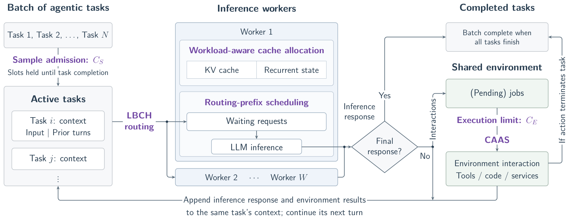
Figure 1. Source [1, Fig. 1]. Each trajectory keeps a sample slot while waiting for either stage. A pending environment job consumes an execution slot when dispatched.
The live evaluation reports 10.4%–65.0% reductions in mean batch makespan across the evaluated model and benchmark pairs. On MCP-Atlas, the move from the tightly gated baseline to the optimized FCFS configuration accounts for most of the absolute savings. CAAS adds a further 3.1% or 8.5% over that stronger configuration, depending on model. I use the reported three-run means throughout. Figures explicitly labeled as examples or calculations are my own.
2. Prerequisites
Two measures of latency
Let sample be admitted at , terminate at , and spend times and in inference and environment service on turn . Queue delays at the two stages are and . For a sequential trajectory, with absent environment stages assigned zero duration, a decomposition is
I take as first task admission when reconstructing the completion curves. The pre-admission wait is part of the batch timeline. TTFT measures how long one request waits for its first generated token. TPOT measures time per output token during generation. Both are sensitive to engine contention and batching. Equation (1) explains why their mean values may worsen while improves. Starting more trajectories earlier can more than offset longer delays on individual calls. It also shows why throughput measured solely during the busy middle of a run is incomplete.
A useful thought experiment is a queue with 100 identical short tasks and one task that calls a tool four times. If the latter is admitted near the end and each tool call yields a new inference stage, the final stage can remain hidden until almost all short tasks finish. Giving it a head start changes the time at which dependent work becomes available. Increasing the tool’s raw service rate is a different intervention. Re-enqueueing a dependent job at the end of a single FCFS queue can repeatedly defer the same chain even if each individual queue decision respects arrival order.
Prefill, latent KV, and recurrent checkpoints
The model needs enough state to resume a cached prefix. Attention layers use stored keys and values or an architecture-specific latent representation. A recurrent layer has a state that summarizes the prefix and advances with a transition at each token. For a schematic recurrence , starting from a saved allows exact mathematical continuation over if the prefix, weights, state format, and position semantics match. Without , the prefix tokens must supply it again from an earlier compatible starting state. This illustrates why a worker with plentiful KV pages can still fail to resume the full hybrid prefix.
Ling-3.0-Flash combines Kimi Delta Attention and Multi-head Latent Attention in the replay setup. The recurrent pool is measured in state slots and the attention pool in KV entries or pages. For strictly advancing, append-only trajectories the design retains the latest reusable recurrent state per trajectory. If a workflow branches from an earlier prefix, rewrites tool observations, or rolls back, the newest recurrent state can become irrelevant to the next input. A shared trajectory identifier remains a scheduling hint in that case. Any actual cache reuse must rely on compatible cache keys and prefix matching.
Separate concurrency units
- Sample concurrency counts admitted and unfinished trajectories. Holding it across queue waits implements a bound on live trajectory state.
- Tool execution concurrency counts nonpreemptive jobs in service. A queued job can retain a sample slot for a long time.
- The inference reference is a capacity model for reusable rollout state across workers. A running decode sequence, an in-flight API request, and an admitted sample are distinct units.
If a tool action expands into several downstream calls, controlling the number of jobs controls downstream load only when job fan-out and retries are also bounded. The paper abstracts each environment stage as a nonpreemptive job with possibly multiple operations. Its simple homogeneous pool is a defensible starting point for their controlled comparisons.
3. Size the two cache pools together
Derivation and sensitivity
Let be the residual memory budget after model weights and non-cache runtime reservations. Write where holds recurrent state and holds KV. The linear system and yields the two individual pool sizes. With a mean final-inference KV footprint and fixed recurrent footprint per trajectory, the continuous estimates in [1, Eqs. 1–4] are
The KV branch decreases with , while the state branch increases. For the state branch is smaller. Moving memory into that branch increases the minimum. For the KV branch is smaller and moving memory back increases the minimum. At equality the optimum of the continuous surrogate follows directly.
The proposed reference for homogeneous workers uses the floor per worker. For two workers with continuous capacity 10.9, the estimate is 20, even though the total bytes would support 21 trajectories if they were pooled perfectly. Runtime reservation, paging, and stranded slack can introduce further discrepancies. Capacity is an estimate of joint residency. Turn timing may permit higher admission; traffic concentrating on one replica may require lower admission.
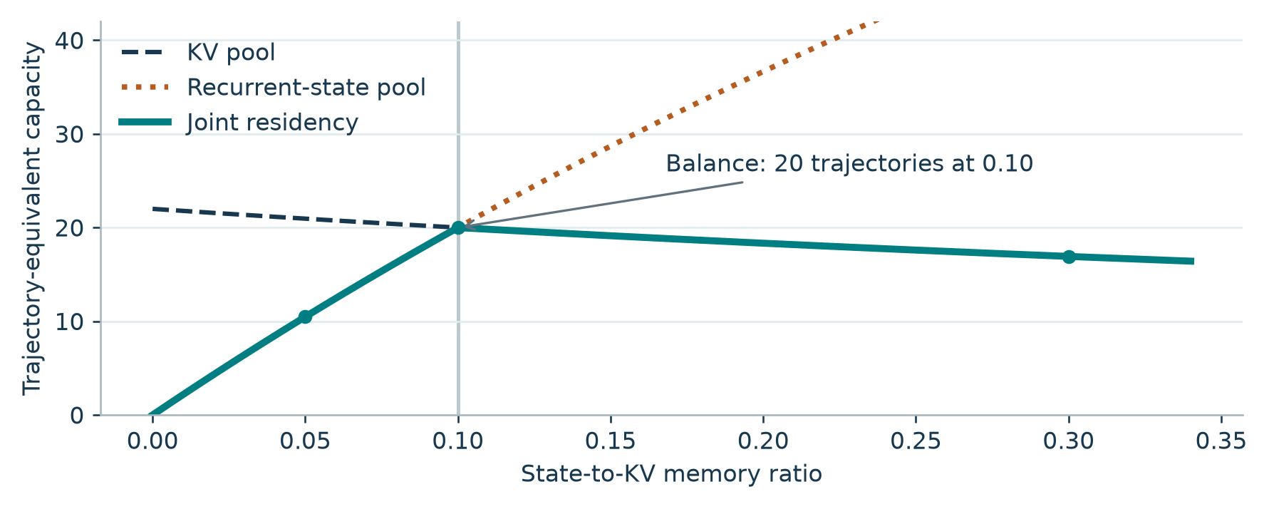
Figure 2. Original illustrative calculation from [1, Eqs. 1–7]. With a 44 GiB cache budget, 2 GiB of KV and 0.2 GiB of state per trajectory, the surrogate peaks at 20 trajectories around ratio 0.1.
For the numbers in Figure 2, at , KV can hold about 20.95 trajectories, but the recurrent pool holds 10.48. At , joint capacity is only 16.92, limited by KV. Doubling a ratio from 0.05 to 0.1 increases capacity far more than increasing the ratio from 0.1 to 0.15. Capacity is continuous through the intersection and has different one-sided slopes. The sign of a small error therefore matters when the two per-trajectory costs are very uneven.
Final-inference means are attractive because a workload can be profiled once and the static partition reused on related runs. A per-request estimator would give disproportionate influence to long trajectories, so the paper takes a per-trajectory mean at the final inference turn. Even that estimate describes the completed workload distribution, while the active population is length-biased. At a random observation time, a trajectory with a 60-second slot tenure is six times as likely to be present as one requiring 10 seconds given equal arrival rates. Some live workloads also accumulate much of their context late in the run.
Recalculating the cost of a stale profile
Assume the workers were provisioned for and the realized mean rises to . Keep the old balance . For , the supported count is . At a new partition the optimum is . Hence the cost of keeping the old split, measured as a fraction of the new attainable continuous residency, is
In the figure’s KV-dominated example, gives 13.33 versus 13.75 at the new optimum. Over-admission against the old reference of 20 is the larger error. For a short-task workload with , the same shift instead leaves the old partition at about 77.8% of the attainable capacity. When , a stale split keeps state as the limiting pool and yields the old capacity; the KV slack remains unused. The effect is asymmetric. The algebra concerns simultaneous residency under homogeneous footprints, and says little about an actual cache-thrashing threshold where timing and grouping matter.
The practical alternative is an allocator that shifts pages between state and KV at runtime, such as the approach discussed in [1, §2]. That reduces dependence on a profile, at the cost of explicit transfer or remapping, allocator complexity, and possible oscillation. A third option is to provision separate worker groups for long and short tasks. It sacrifices pooling flexibility and requires a workload classifier, but keeps extreme footprints from influencing every worker’s fixed partition.
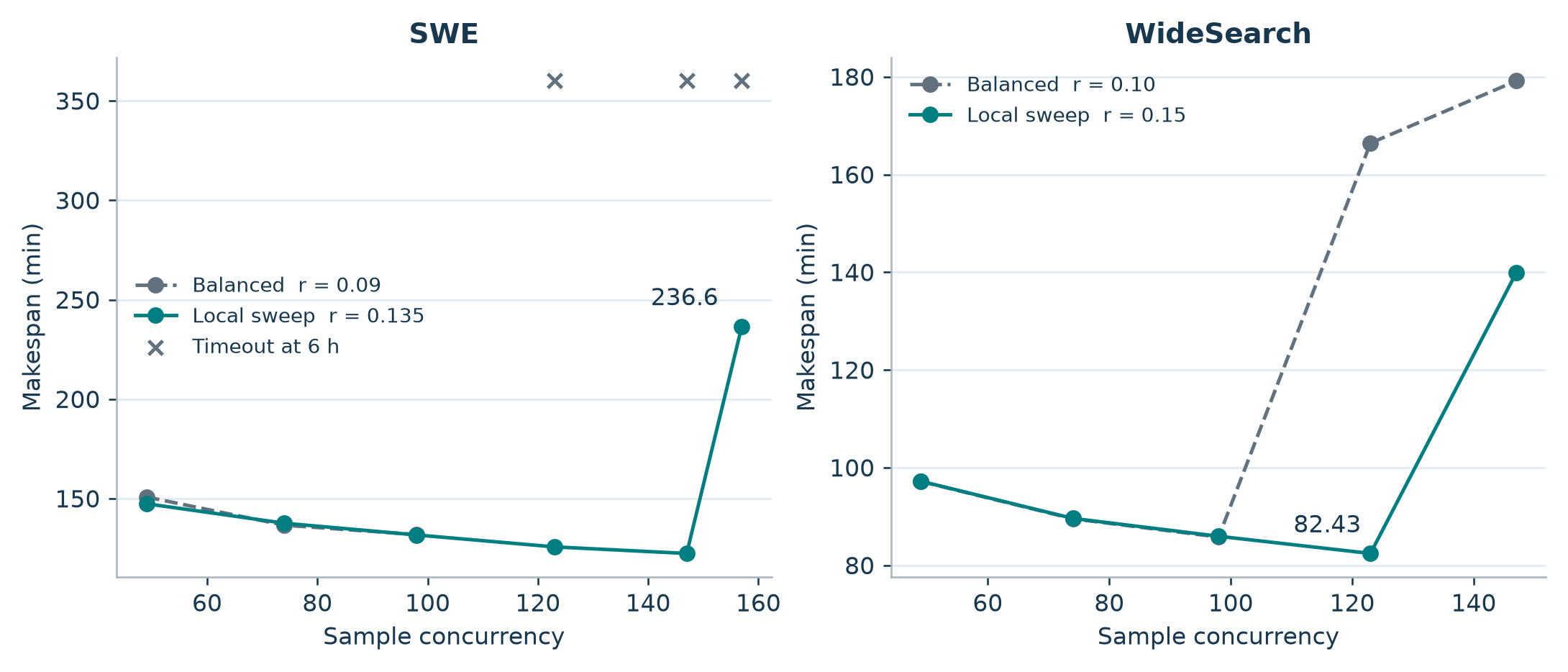
Figure 3. Redrawn from [1, Fig. 3], SWE and WideSearch rows only. The markers show timed batch makespans. Timeout cells are omitted from lines and annotated with their six-hour censoring.
On SWE, the balanced point , records 131.9 minutes. The local minimum shown is 122.4 minutes at , . Moving from 147 to 157 at the latter ratio jumps to 236.6 minutes. In WideSearch, reaches 82.43 minutes at 123 and 139.90 at 147. The paper reports roughly eleven-, three-, and ninefold increases in new-prefill work around the highlighted SWE, BFCL, and WideSearch transitions. These sharp changes favor a small local sweep that includes timeout detection and eviction counters over optimizing an unconstrained smooth curve. BFCL adds a complementary caution: the measured best ratio 1.13 is below the predicted 2.26, with corresponding sample concurrency 644 versus the reference 859. The optimum depends on traffic and execution as well as memory division.
4. Route turns without losing their history
The gateway sees requests from many trajectories, each identified by a stable label. With a fixed worker ring, deterministic hashing maps the same label to the same home. A cold worker can reconstruct the prefix, but in this setup it cannot pull the other worker’s complete hybrid state. Large correlated bursts assigned to the same home make pure consistent hashing expensive. The paper adapts bounded-load hashing [2] using the current number of queued or running inference requests as the load signal. For workers the candidate test is
The new request enters the numerator. The current load on the proposed worker enters the left-hand side. This test can yield a post-assignment load above , so the rule is an eligibility threshold on observed load. A small threshold yields load-sensitive spillover; a larger one admits more skew in exchange for affinity. With counts , , and , the threshold is 5. A home at load 8 spills to the first clockwise eligible replica. The paper evaluates on two workers; neither the threshold nor clockwise selection uses cache-transfer costs or estimates of remaining tokens.
Algorithm 1. Load-bounded consistent hashing
Adapted from [1, Algorithm 1]. Observe loads once for the routing decision.
1. Hash the trajectory label onto the worker ring.
2. Take its first clockwise worker as home.
3. Compute the threshold from total in-flight requests plus one.
4. Visit home, then each successor clockwise at most once.
5. Return the first worker whose current count meets the test.
6. If none meets it, return home.
With exact counts for a nonempty ring and , some worker has load at most the mean, and the mean is below or equal to the threshold. The defensive fallback remains relevant when operational eligibility includes an additional filter or counts are observed inconsistently. Further replication increases the potential scan length. More importantly, count skew is an imperfect measure of cost skew. One cache-cold 200k-token prefill can be more expensive than many nearly cached short requests. Smoothing a count, scoring estimated uncached prefill plus decode work, and giving local affinity a byte- or time-based benefit are plausible alternatives. They require telemetry, a prediction horizon, and a policy for stale estimates.
If a long trajectory spills for several turns, its dependencies are still serialized through the runner. The hash continues to point to the original home. A subsequent turn that returns may find the home holds an older prefix than the spill destination. Keeping an explicit last-worker hint could avoid this when the spill replica remains healthy. It could also trap an unlucky workload on a saturated worker. I would compare the two by logging the age of the newest compatible state on a sampled subset of routing decisions.
Algorithm 2. Routing-prefix scheduling
The worker keeps an LRU of recently admitted trajectory labels with capacity . It reads the prefix cache once per queued request when the label first qualifies for the first tier. Let be that recorded hit length and its enqueue time. Sort in ascending lexicographic order:
1. For each waiting request, test its label against the recent set.
2. For a recent label with no recorded hit, query the radix cache.
3. Save that hit length for later scheduling rounds.
4. Compute the two-tier priority key and sort the waiting queue.
5. Give that order to the resource-constrained batch builder.
6. For each admitted request, move its label to most recent.
7. Trim the set to its capacity and return the admitted batch.
The underlying batch builder still respects token and memory limits. A recent label can have a short or zero hit and still outrank a cold-tier request. In [1, §3.3] the prose specifies a capacity of and up to retained labels. I interpret the update as trim after appending and moving the label. The typeset expression puts the tail operator before the final append, which could keep entries if followed literally. The distinction is testable with a two-label set of capacity two. The default is the floor of the model-derived worker residency, a scale for the number of recently useful trajectory labels.
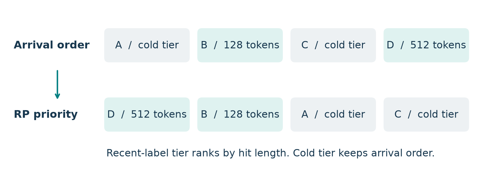
Figure 4. Original example from [1, Algorithm 2]. B and D have recent labels and are sorted by recorded hit length. A and C keep chronological order in the second tier.
The cache and the label set have separate clocks. Eviction after scoring makes the stored hit optimistic, while eviction before scoring can leave a recent label with a true zero hit. A label can also expire while its GPU state survives. Those are priority errors; the server still has to use the eligible state at execution. A full LPM pass can react to newer residency but repeatedly searches long prefixes. DFS-weight also traverses the cache structure. In rough accounting, for queue sizes across scheduling rounds, in the paper’s priority policy the number of prefix queries is bounded by the number of distinct waiting requests that ever enter the recent tier. The key assignment and sort still incur costs for each round. Selective matching and memoization reduce cache lookup work while the full queue sort remains on the scheduling path.
The replay table makes this tradeoff concrete. At SWE , priority computation totaled 735.00 seconds for LPM, 1704.25 for DFS-weight, and 303.05 for routing-prefix. At BFCL the values are 7.65, 172.15, and 10.91 seconds. LPM often fell back to FCFS past a queue length of 128. Its smaller priority-computation total in that condition comes with 34.0 minutes batch time versus 19.8 for RP. Cumulative priority time is not necessarily additive to end-to-end waiting. The worker can overlap scheduling and GPU work, and changed schedules can cause additional batches and prefills.
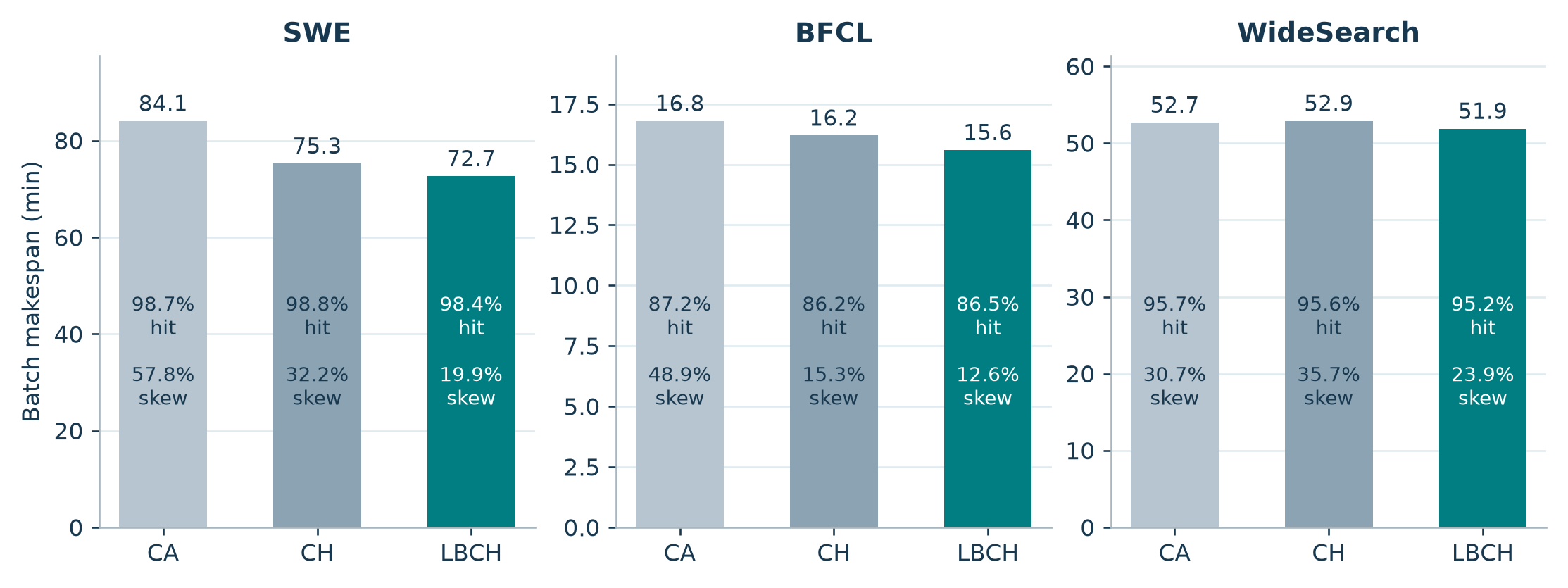
Figure 5. Redrawn from [1, Figs. 8–10]. All runs use two TP4 workers and RP. The highlighted makespan differences coexist with similar cache reuse.
Once a workload is already above 95% cached tokens, small changes in cache hit rate can coexist with substantial changes in which worker becomes the straggler. The paper’s time-averaged count imbalance and token imbalance can be read as
Here counts in-flight requests and counts generated tokens. For two equal 10-second intervals at counts then , is . A further interval at does not enter . This convention prevents a long single request from mechanically assigning extreme count skew to a router, but also removes part of the tail that determines makespan. weights total output tokens, regardless of whether batches ran efficiently or how much input each worker had to recompute. On replay SWE, count skew falls from 57.8% under CA to 19.9% under LBCH and batch time falls 84.1 to 72.7 minutes. Live WideSearch with Ling-3.1 goes the other direction on count skew, 8.8% to 17.6%, while makespan still improves. These measures explain parts of the trace under a controlled comparison; the live bundle can change several factors at once.
5. Keep the tools busy and advance the batch tail
With a single application gate, admitted samples cannot exceed both the inference reference and environment capacity. Separating gates lets waiting trajectories queue ahead without starting extra tool jobs. The two defaults in [1, Eqs. 11–12] are
An intuition comes from an idealized alternating service model. Suppose every turn consumes mean time on one of equivalent inference slots and on one of environment slots. Ignore queues and batching for this calculation. By conservation of service effort, the stage-cycle rate cannot exceed either stage’s capacity. The active sample limit also bounds the rate because each cycle takes at least its own service time on average.
For , , s, and s, a unified gate at 3 bounds the rate at 0.375 cycles/s. At the environment ceiling of 0.5 cycles/s can already bind. This argument ignores precedence bunching, memory behavior, and batched inference, so the calculation provides a bound for the toy model rather than a model of H20 performance. It explains why the gain can flatten much earlier than the inference cache reference would predict. In MCP-Atlas replay at fixed , increasing to 10 from 3 or 5 reduces makespan by about one third. The change from 25 to 50 moves it much less, as mean in-flight inference barely changes.
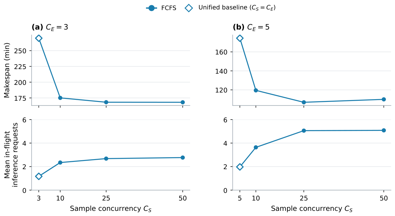
Figure 6. Source [1, Fig. 11]. Each panel holds tool execution capacity fixed and varies only sample admission under FCFS. The leftmost point uses the unified gate.
Algorithm 3. Chain-Advancing Action Scheduling
For pending job , is the slot-request time, the completed inference turn count, the mean of those turns’ observed durations, and its globally increasing enqueue sequence. The parameters and are respectively the arrival band width and the inference-duration bucket width. The key in [1, Eqs. 13–16] is fixed when the job arrives:
1. When a trajectory requests a tool slot, record arrival and depth.
2. Compute mean observed inference time and its integer bucket.
3. Attach the arrival band and a strictly increasing sequence.
4. Insert the job into the pending queue using the fixed key.
5. When a slot frees, pop the minimum key and start the job.
6. On return, finish the sample or release its next inference turn.
One can maintain a running sum and count of inference durations so that step 2 costs constant work per arrival. A min-heap gives logarithmic insertion and selection in the number of pending jobs. The algorithm in the paper is an ordering rule, independent of the choice of queue data structure. It does not preempt running jobs. The arrival band prevents a deep chain from overtaking work in a strictly earlier band. Within a band it may move ahead of a shallow job that has waited slightly longer. With s, tickets at seconds 29.9 and 30.1 land in separate bands even though only 0.2 s apart. Tickets at 0.1 and 29.9 can be reordered. Neither property bounds total wait unless arrival, service, and admission also meet capacity assumptions.
The observed depth is a proxy for residual critical-path length. If deeper stages predict longer remaining work, promoting them reveals future work early. If stopping times are memoryless, depth alone carries no residual-length information. Workflows with an initial discovery phase followed by a single long tool call could even reverse the relationship. The third key component is an estimate of the next inference return, based on past per-turn duration after band and depth agree. It may improve worker feed when timings are predictive. Cumulative context growth, changes in cache hit, or a mixed workload can make it misleading. Bucketization limits sensitivity to timing noise and leaves stable FCFS ties.
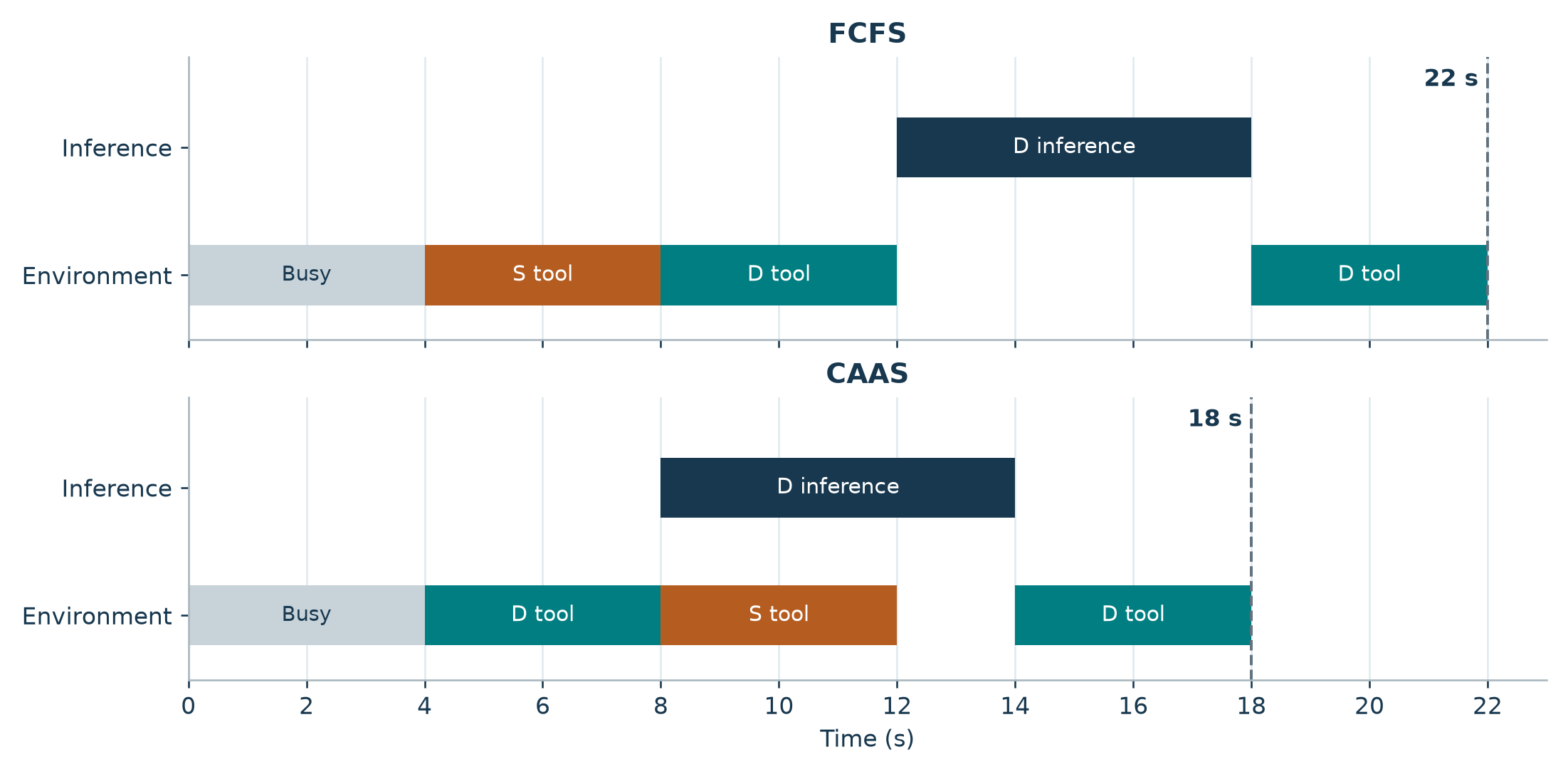
Figure 7. Original toy timeline. One tool slot opens at time 4. Both queued jobs are in one band. D has deeper observed progress and six seconds of subsequent inference. Makespan in the constructed schedule moves from 22 to 18 seconds.
In the example, FCFS dispatches shallow S at 4 and deeper D at 8. D returns at 12, runs inference until 18, and occupies the tool again until 22. With CAAS, D first returns at 8. S uses the environment from 8 to 12 while D runs inference until 14. D returns from the final tool at 18. Tool service work for S and D is 12 seconds under either policy, and there is no change to model or tool output. The gain is four seconds from moving otherwise serial work into overlapping intervals. If S instead releases a long final inference stage, reprioritization can increase . I would compare this policy to FCFS, depth-only ordering, and a predictor that estimates residual work with an age cap. A predictor needs calibration data and changes the maintenance burden; banding has a smaller input contract.
6. What the experiments establish
Replay fixes dependencies and lengths, while still running the model
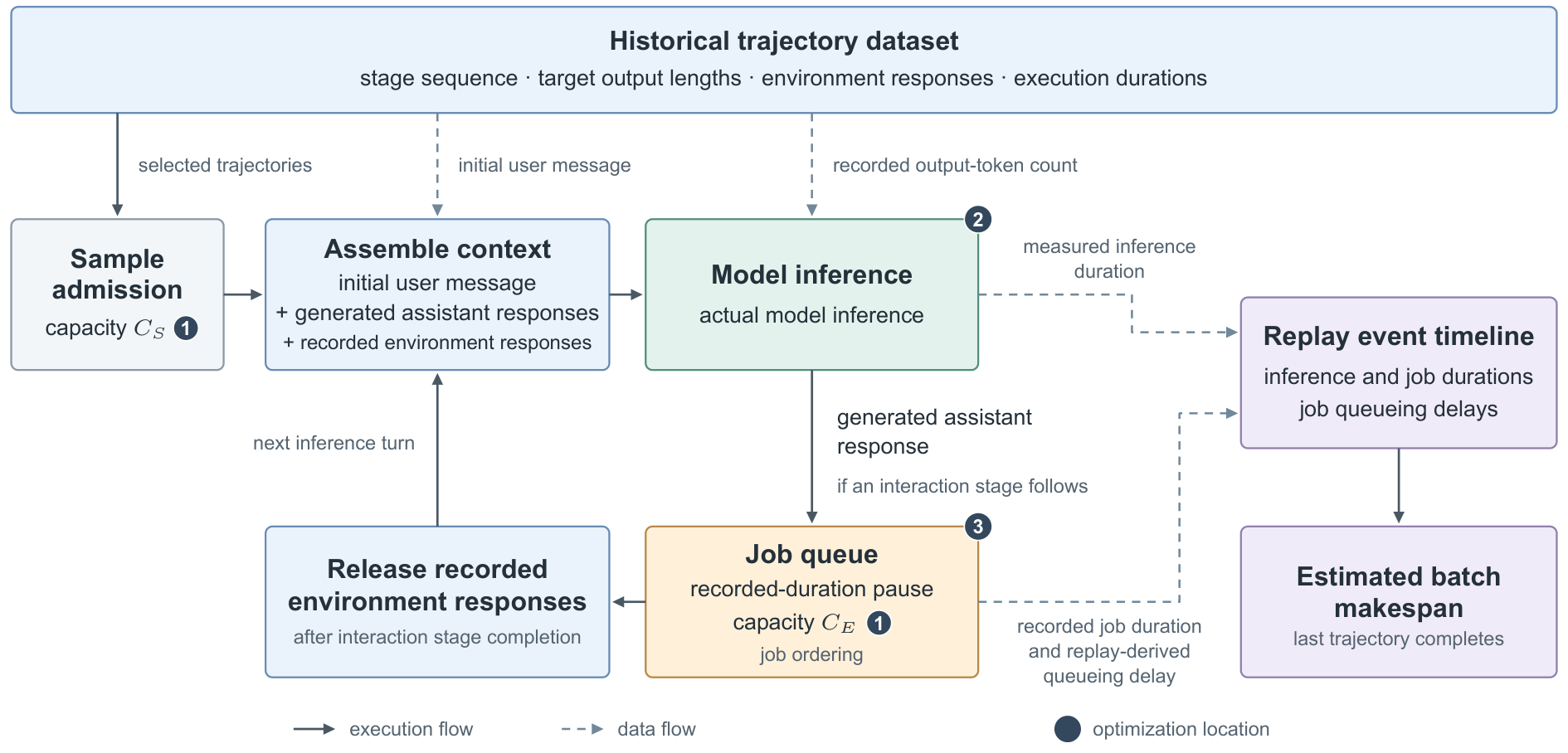
Figure 8. Source [1, Fig. 2]. A completed replay job releases a recorded observation after a timed wait. Live inference generates the turn’s prescribed token count.
The authors replay actual model inference on H20 with one or two TP4 workers depending on the comparison. Each trajectory has a recorded stage sequence, initial prompt, target output lengths, tool result text, and tool service durations. The input includes newly generated responses from earlier replay turns and recorded tool results in execution order. The framework pauses for the recorded service time after a job acquires a slot. The generated response can propose a different action than the one in the trace. This design isolates cache, batching, dispatch, and queue interactions under the same demand trace. It breaks feedback from the chosen action to its actual environment response, retries, and future trajectory length.
Inference-only replay omits tool capacity and delays. The 289 SWE traces were successful historical trajectories, with 25,416 inference requests. BFCL supplies 5,106 traces and 17,029 requests, and WideSearch supplies 200 traces and 5,672 requests. Dividing requests by trajectories yields about 87.9, 3.34, and 28.36 requests per trajectory, respectively. These are sample means over the selected traces. They help interpret why concurrency and caching matter differently across workloads. For coordination, the 495 MCP-Atlas replay traces also come from successful historical runs. This cohort excludes some retry and failure dynamics that the live evaluation includes.
The most informative contrasts hold the following elements fixed:
| Question | Fixed within replay | Reported contrast |
|---|---|---|
| Which cache partition and admission level? | One TP4 worker and FCFS | Joint sweep, including timeouts |
| Which worker queue policy? | One worker and balanced ratio | FCFS, LPM, DFS-weight, RP |
| Which gateway policy? | Two workers, RP, ratio and sample cap | CA, CH, and LBCH |
| Does independent admission help? | Environment limit and FCFS dispatch | Unified cap vs 10, 25, and 50 |
| Does action priority help? | Sample cap 50 and same environment limit | FCFS vs CAAS |
In the final replay comparison, changing only job order cuts makespan by 1.9% at and 3.5% at . The final 5% interval shrinks by 19.0% and 21.4%, respectively. The CAAS curves reach 95% later while reaching 100% earlier. This directly illustrates a distributional tradeoff. There is no requirement that a batch-optimized scheduler stochastically dominate FCFS at every completion percentile.
Matched admission in live SWE
The live setup uses two TP4 workers for Ling-3.0-Flash and two TP8 workers for Ling-3.1-Flash, all on H20 GPUs. The paper gives three-run means and fixes checkpoint, task IDs, sampling settings, and hardware within each model and benchmark comparison. There are three useful versions of live SWE. Baseline-1 is an empirically tuned admission limit using the original cache and worker policies. Baseline-2 raises admission to the same level as Opt without changing those policies. Opt changes all three inference-side components as a package.
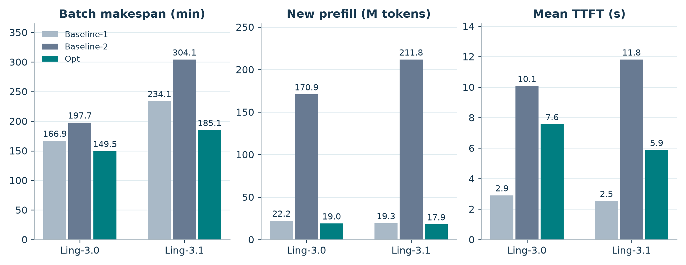
Figure 9. Redrawn from [1, Table A3]. Baseline-2 and Opt have matched sample admission. Baseline-1 uses lower admission and has the smallest TTFT in each model block.
For Ling-3.0, raising admission from 100 to 250 under baseline policies increases makespan 166.9 to 197.7 minutes and uncached prefill 22.2 to 170.90 million tokens. At 250, Opt cuts uncached prefill to 18.98 million and finishes in 149.5 minutes. For Ling-3.1, raising admission from 50 to 100 increases makespan 234.1 to 304.1 minutes, and new prefill goes from 19.3 to 211.81 million. Opt at 100 returns new prefill to 17.93 million tokens and ends at 185.1 minutes. Directly dividing the A3 values gives 88.9% and 91.5% less uncached prefill relative to matched-admission baselines. Table 2’s hit percentages and token sums are separately averaged and rounded. Multiplying those rounded means gives an approximation to mean uncached tokens. Table A3 is the better source for the measured means.
TTFT illustrates the choice of comparison. On Ling-3.0, Opt is 7.57 s versus matched Baseline-2’s 10.08 s, but tuned Baseline-1 averages 2.90 s. On Ling-3.1 the corresponding values are 5.88, 11.81, and 2.54 s. Opt improves batch time and recovers much of the high-admission latency loss. An interactive service that values request latency would care about the comparison to Baseline-1 and the latency distribution. The averages alone are insufficient to certify a percentile SLO. Live WideSearch adds summarization by the evaluated model and does not reproduce the replay cache totals. BFCL-v4 is omitted for Ling-3.1.
MCP-Atlas and the denominator behind the percentages
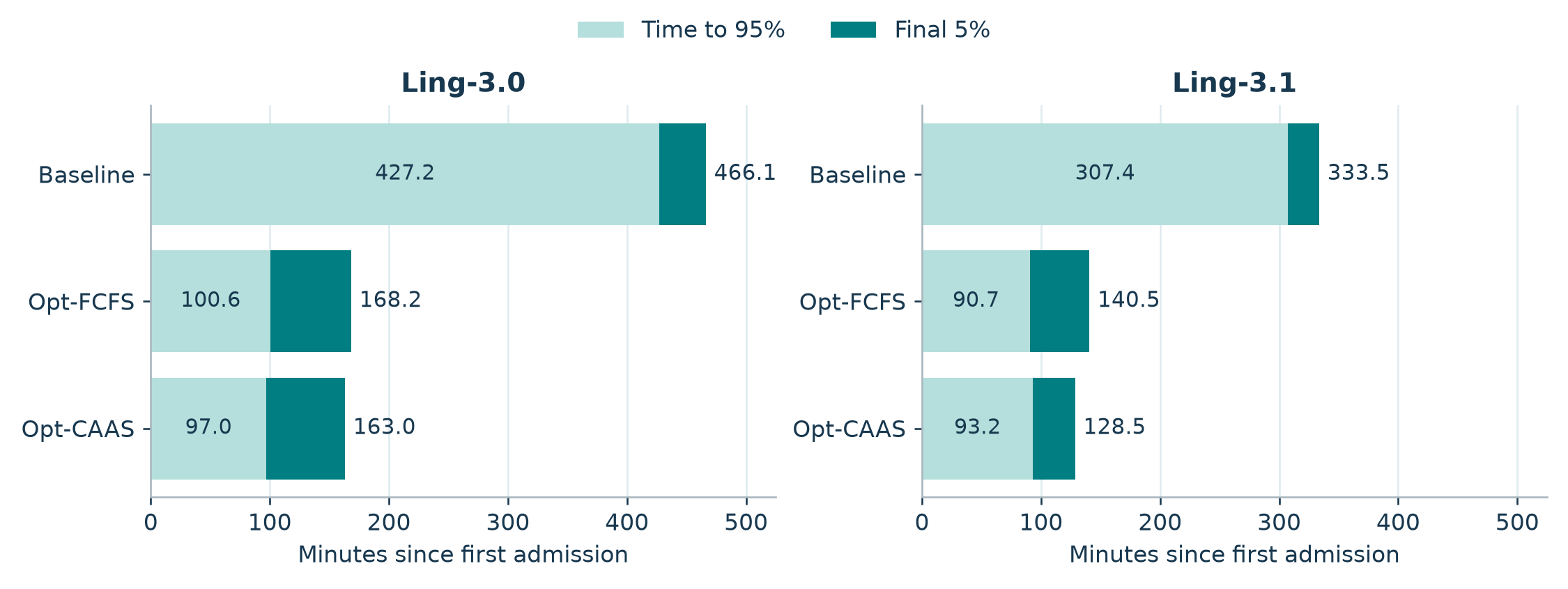
Figure 10. Redrawn from [1, Table 3]. The pale part of each bar is the implied time to 95% completion and the dark part is the last 5% interval. Both use minutes since first admission.
Let be the time at which completion fraction first reaches . Termination includes failure in Table 3. The authors’ definition gives
For a fixed task count, subtracting the mean from mean makespan gives mean exactly up to input rounding. I obtain 427.2, 100.6, and 97.0 min for Ling-3.0 across baseline, Opt-FCFS, and Opt-CAAS. For Ling-3.1 the values are 307.4, 90.7, and 93.2 min. On the latter model, CAAS reaches 95% 2.5 minutes later than Opt-FCFS, saves 14.5 minutes in the remaining interval, and ends 12.0 minutes earlier. On Ling-3.0 it reaches 95% earlier as well. The shape of this distributional shift is workload- and model-dependent.
The live environment limit is 3 in all three MCP-Atlas configurations. Opt-FCFS changes from 3 to 50 and simultaneously changes the inference setup. It accounts for 297.9 of the 303.1 minutes saved end to end on Ling-3.0, and 193.0 of the 205.0 minutes on Ling-3.1. Those are 98.3% and 94.1% of the absolute baseline-to-final time savings on a sequential decomposition. CAAS supplies the remaining savings. The individual percentage changes multiply when expressed as time ratios with successive denominators; adding the percentages of the two reductions would overstate the total. Experimentally, the Opt-FCFS to Opt-CAAS step holds the optimized settings fixed; the baseline step bundles several mechanisms.
On both models Opt-CAAS has a longer final 5% interval than unified baseline, even though both and makespan are much earlier. Broad admission lets short tasks finish well before the long trajectories. The paper reports mean turn counts among the last 25 under Opt-CAAS of 27.9 and 15.6 versus 10.1 and 7.9 in baseline, and checks task-ID overlap against baseline lengths. A short tail interval in a slow baseline can arise from which samples were admitted late. One can improve the whole completion trajectory substantially while leaving a subset of long tasks as a larger fraction of remaining runtime.
7. Limitations
Replay excludes failed historical traces in the stated SWE and MCP-Atlas cohorts and prescribes a fixed service time for each environment job. It can estimate the mechanical consequences of a scheduling change under a trace. In live services, job order can change HTTP rate limits, burstiness, tool retries, and the text returned. Optimizing against successful historical traces may underestimate expensive trajectories with repeated retries. The paper’s live makespan includes retries and eventual failures, which helps address this weakness, but leaves the competing dynamics entangled.
The population of benchmarks, two Ling versions, and H20 deployments constrains generalization. The cache ratios depend on architecture, allocator, numerical format, hardware, and observed workloads. The choice of s and s is fixed for the reported coordination experiments. A GPU pool at a different efficiency or an environment with strongly heterogeneous jobs may favor different settings. Tail means are reported without paired uncertainty intervals, and the average benchmark scores support plausibility of retained quality without providing a statistical equivalence test. For example, the Ling-3.0 live Opt-FCFS to Opt-CAAS score changes from 66.6 to 65.6; per-task paired results would show whether this difference is compatible with the chosen quality margin.
8. Critical analysis
Test whether depth is a predictor of what remains
A deeper observed chain has survived more turns. Whether that raises expected residual work depends on the stopping distribution. For a discrete total turn count , among trajectories that survive to turn , the expected remaining length can be written as a sum of conditional survival probabilities.
The first equality expands a nonnegative integer as a sum of its threshold indicators. For a geometric stopping law the ratio is independent of , yielding no depth signal. For a mixture with 80% two-turn tasks and 20% twelve-turn tasks, the expected residual at is . At all survivors come from the long class and the residual is 9. At it drops to 1. CAAS is sensible in the first part of this example and overly optimistic about depth near the end. In a batch with two-turn tasks that have much longer tools, task depth can also rank the wrong resource demand even when it predicts remaining turns.
I would estimate residual wall time and remaining chain length stratified by observed depth, workload, tool class, and whether previous calls retried. I would also measure the chance that the next release produces a ready inference turn. A policy using residual quantiles under an age limit is a good test of how much improvement the simple depth rule leaves. A deadline or age cap should be evaluated on the joint makespan, tool-queue tail, and request SLO instead of through a single regression fit.
Give replay a second axis of stress
A useful extension holds the same task IDs and prompts, then repeats the comparison at matched with technology-specific dispatch ablations. I would add correlated service delays by tool endpoint, bursts of transient error, and a pool with a rare slow tool that consumes most of the service time. In a two-resource system with total tool job seconds and equivalent slots, is a lower bound on makespan, where is the sum of service times on trajectory and ignores all waits. The standard work and critical-path bounds follow from integrating available parallel capacity and following serial dependencies, respectively. Neither bound predicts the actual schedule, but plotting the gap to each reveals whether optimizations help even in a trace near the environment work floor. If tool classes have independent ceilings, the maximum of their individual work bounds is more informative than pooling every job into one class.
I would report remaining samples over absolute time along with and . Matched task IDs support comparing per-task completion times and checking whether improvements disproportionately benefit a specific subset. Paired batch repeats, or a block resampling design respecting shared rate-limit bursts, would add uncertainty intervals without treating every tool action as an independent sample. Counting the tasks run to failure alongside the score avoids an apparent makespan improvement caused by earlier failures. A noninferiority assessment needs a specified score margin and enough repeated evaluation to estimate its uncertainty.
How much of this design is needed with FlashStates?
A shared cache budget changes the deployment problem in §3. With FlashStates [6], attention KV and recurrent checkpoints draw from one GPU cache budget. The fixed ratio and its workload-specific sweep can go away. A first estimate of residency can still use the combined footprint in Eq. (3). In practice, the sample admission limit still needs calibration because live allocations, shared KV blocks, and the cost of evicting reusable states all affect how far concurrency can be raised.
Routing-prefix scheduling is the next mechanism I would test for removal. If FlashStates’ retention policy keeps an intact hybrid state until the next turn returns, the worker has less to gain from moving that request up the queue to save its cache entry. Preferring a hot request may still change batch composition and TTFT. Cross-worker routing addresses a separate source of lost reuse. With worker-local caches, a turn sent to another replica can lose access to the cached prefix. Load-bounded routing can still trade affinity against worker imbalance.
At the environment layer, I would start with separate sample and tool limits and FCFS dispatch. A better cache can reduce inference time between tools and thereby change when jobs arrive. Tool quotas and the order in which jobs release the next inference turn still matter. CAAS is worth testing when a constrained tool queue and long sequential trajectories continue to dominate the tail. Table 3 isolates its incremental gains with the paper’s original inference stack. The two papers leave its incremental benefit on FlashStates unmeasured.
A minimal comparison would hold the model, hardware, total cache budget, task set, arrival order, and tool limit fixed. Start with FlashStates and separate limits, then test RP alone, CAAS alone, and both together. On a multi-worker deployment, compare the two routing policies in a separate sweep. I would first match sample admission to isolate policy effects, then tune the admission cap for each stack to compare its best operating point. Report uncached prefill, time waiting for tools, time to 95% completion, and final makespan. That would show which mechanisms still improve the batch after removing the fixed split.
Joint admission at the point where queues start to grow
The static cache calculation is a credible initializer. A robust gate could use measured eviction or new-prefill rates, context quantiles among active trajectories, and delayed feedback from the tool queue. Reducing when the environment is saturated can relieve memory pressure even when GPUs occasionally idle. A controller with hysteresis or minimum dwell time would avoid oscillating between cache thrash and underfill. To show whether it adds value, the comparison should include a tuned static at each arrival mix and a cached-state footprint measurement, controlling for task composition and total service budget.
Each worker could also expose measured prefill debt and retained-state pressure to the router. Replacing count with debt is appealing for heterogeneous prefills, but transferring active trajectory state or over-spilling can itself add delay. Two diagnostic counters would help disambiguate the mechanism: the fraction of spilled turns that lose the latest checkpoint, and the amount of actual prefill work lost to the spill. For RP, label-tier age and hit-estimate age can be logged to test bounded aging and epoch invalidation. An eviction-aware invalidation that triggers only on relevant cache mutations could keep the cheap common case without preserving stale reuse estimates indefinitely.
9. Reproducing the comparisons
For a budget-matched reproduction, start with the settings in [1, Appendix A]. Inference-only replay uses thinking-enabled Ling-3.0-Flash with four-way tensor parallelism per worker. The routing experiment spans , , and for SWE, BFCL, and WideSearch. The coordination replay uses two TP4 workers, ratio 0.14, for FCFS versus CAAS, and both and 5. The live MCP-Atlas setting is with for Opt, and baseline is 3 for both. The live optimized ratios 0.14 and 0.34 reflect different models. Capture checkpoint, tokenizer, runtime flags, dataset splits, upstream service constraints, and retry rules at the level that can explain deviations.
At minimum retain timestamps for admission, each inference enqueue and completion, each environment enqueue/start/end, and final task termination. Log labels and cache hits in aggregate or through anonymized trace IDs, and keep identities stable across comparisons. Validate trace conservation: no scheduled environment job starts without an available slot, a sequential trajectory has at most one outstanding job, and environment completions release exactly the recorded successor or termination. In inference replay, match token totals and warm-up treatment. In live runs, keep all outcomes and attribute changes in overall makespan alongside any change in success rate or retries. Timeouts in the cache sweep are censored data and need a distinct reporting path.
For this review I recalculated the pool balance, routing and timeline examples, completion quantiles implied by Table 3, and durations and percentage changes from Tables 2–3 and A3. Those are arithmetic checks and illustrative schedules. The empirical measurements belong to the paper.
10. Conclusion
The paper shows where a serving policy can shorten the dependency chain seen by downstream batch workflows. Its evidence is strongest when both pool residency and cross-stage occupancy are measured, the task set is held fixed, and CAAS is compared to FCFS with the same admission and environment limits. Higher admission buys overlap until the cache or environment becomes the bottleneck. Routing and local scheduling can postpone the cache cliff, while environment priority can expose more of the long chain before the batch runs out of parallel work. A deployment should evaluate both final completion and the spread of task and request latencies, especially when the same engine serves interactive traffic.
References
- Feng et al. (2026). Reducing Batch Makespan for LLM Agent Workloads through Inference–Environment Coordination. Versioned text, PDF. Figures 1, 6, and 8 here are cropped from the CC BY 4.0 paper. Figures 3, 5, 9, and 10 are redrawn from its data.
- Mirrokni, Thorup, and Zadimoghaddam. Consistent Hashing with Bounded Loads.
- Zheng et al. SGLang. Pan et al. Marconi.
- Bandi et al. MCP-Atlas. Khandpur et al. SWE-bench Multilingual.
- Ling Team. Ling-3.0-Flash and Ling-3.1-Flash model cards.
- Li, Xu, Zhang, Wang, Zhou, and Xu (2026). FlashStates: Unlocking Flexible Hybrid State Management for Agentic LLM Inference.