Review date 2026-11-14
Author Zhongzhu Zhou
Paper reviewed Spectral Rank and Step-Direction Dynamics in Language-Model Post-Training
Paper authors Khurram Khalil and Khaza Anuarul Hoque
arXiv 2611.11752
Version and date v1, 2026-11-09
The three measurements
Khalil and Hoque ask how post-training moves a language model in weight space. Their study uses three objects. A matrix difference between an initialization and an endpoint has a singular spectrum. A sequence of intermediate checkpoints supports correlations between finite displacements. Finally, a paired training intervention asks whether changing the way advantages are computed changes those correlations. The three objects have different denominators, units and sources of uncertainty. I found that keeping them in view together makes the paper much easier to read.
The practical trap is to see a small number labelled “rank” and budget a rank of that size for compression. In the selected OLMo-2-7B PPO attention query at layer zero, the paper reports stable rank 9.58 and 532 directions for 80% of the squared update energy. The second trap is to interpret the angle between two saved displacements as the angle between two optimizer updates. The public 7B PPO example compares finite windows of 60 release steps. The third trap is to treat a small, matched training experiment as an explanation of the entire public survey. Replacing group-relative advantages with a critic–GAE package makes the mean late cosine smaller in the matched study. The production pattern of consistently negative adjacent cosines remains a separate observation.
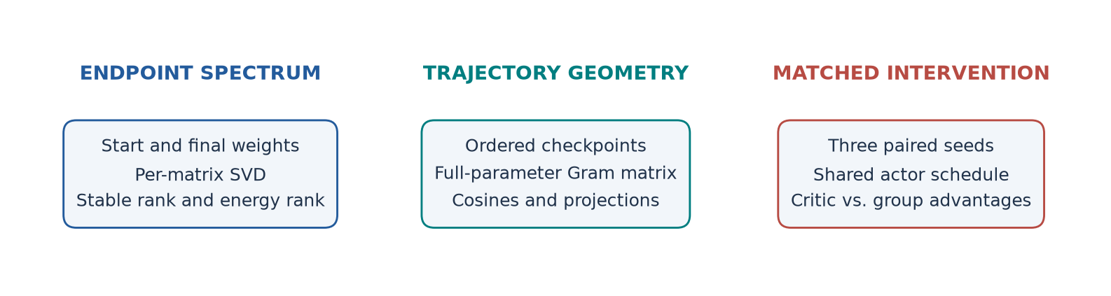
Figure 1. Original schematic based on paper §§2–4. The endpoint uses one matrix difference, the trajectory uses a full-model checkpoint grid, and the intervention pairs training runs by seed.
What the paper establishes
The analytic result is a separation between stable rank and fixed-energy rank for a family of singular spectra. The observation from fourteen full decompositions is that these measures can be far apart for actual post-training updates. The survey then records negative adjacent cosines in every measured pair across nine public stage trajectories. Finally, the matched 1B intervention detects a drop in mean late-window cosine when the advantage package changes. These statements are respectively a theorem, a selected-case measurement, a descriptive survey, and an intervention in a specified setting. The paper’s numerical appendix is unusually relevant to all four: it documents a corrected initialization, a discarded coordinate sketch, sensitivity of threshold rank to approximate SVD, and the limits of the original controlled comparisons.
The rest of this review uses my own equation numbering. Results from the paper are identified by its table, section, or appendix. The power-law sum, small vector examples, and arithmetic checks are my calculations. I did not run a model-training or task-evaluation experiment for this review.
Prerequisites
The model and the stage boundary
An endpoint difference is a statement about two objects that share a parameterization. For a layer with weight shape by , the change is obtained by matching the same layer name, orientation, tensor dimensions and coordinates. In a weight-tied model, a full-model norm should include each independent parameter once. One-dimensional normalization weights contribute to the trajectory norm even though the per-matrix SVD study excludes them. A transposition preserves singular values, but it changes what the left singular vectors describe. That matters for the separate angle calculation on weight subspaces.
A model may go from a base model to supervised fine-tuning (SFT), then direct preference optimization (DPO), then reinforcement learning from verifiable rewards (RLVR). SFT trains on given conversations. DPO uses a fixed pair of preferred and dispreferred responses. RLVR samples responses from the evolving policy and scores them with a verifier. For the public OLMo-2-7B PPO endpoint, the immediate reference is DPO. For the author-run SFT endpoint, the reference is the corresponding base checkpoint. The spectra compare two kinds of endpoint in the paper’s setting, for which the objectives, exposure, reference and horizon all differ.
Let , and be the SFT, DPO and RLVR endpoint matrices. Inserting the intermediate checkpoint gives
This identity is linear in weights; singular values of the sum depend on both spectra and their orientation. If the two changes use the same leading left and right directions, they can add or cancel. If their supports in both singular bases are disjoint, the sum can carry both spectra. For interior trajectory differences, subtracting the same reference from both endpoints cancels exactly in real arithmetic. The first window can still change because a different initial checkpoint changes the window itself. Subtract the source values after widening storage precision when small differences are the quantity of interest.
SFT, PPO, group-relative advantages and GAE
The SFT runs in this paper supervise all retained non-padding conversation tokens that have a preceding token. A response-only SFT run changes that mask and can move weights differently. The normalization divides by the number of supervised tokens. At a fixed example count, tokenization and length can still change how many gradient terms the model sees. The cross-family benchmark matches 64 examples per optimizer step and a common schedule, with token exposure left model dependent.
For RLVR, an advantage assigns credit or blame relative to a baseline. Proximal policy optimization uses a token probability ratio between the current policy and the policy used when sampling. For positive advantage, the clipped objective stops rewarding a ratio increase after the upper clipping bound. For negative advantage, the incentive to decrease the ratio saturates at the lower bound. The product uses the same sampled action under both probabilities. The reference-policy penalty and several passes over a rollout add further dependence on past parameters and sample reuse. Displacements therefore reflect the optimizer, the rollout and the training schedule as well as the objective. The public stage labels refer to released training recipes. The two local arms deliberately share a clipped actor objective, so I refer to them by their advantage packages.
For group-relative advantages, the paper standardizes the eight outcome rewards for each prompt with their population standard deviation and a stabilizing constant. It broadcasts one standardized value to all retained tokens in a response. For a binary reward group with exactly one success and seven failures, the mean is and the population standard deviation is . Ignoring the stabilizer for this example, the success receives and a failure receives . Their response-level sum is zero. Longer trajectories still occupy more terms in the token-weighted actor objective, and a response without EOS can receive a different reward in the paper’s protocol.
The critic estimates a state value . Using reward , discount and trace decay , the paper first forms a temporal-difference residual and then accumulates residuals backward from the terminal token. Let index the terminal token and set its successor value to zero.
Separate the first term of the sum and factor out to get the recurrence. When , the intermediate value terms telescope and the residual sum reduces to the discounted return less the starting value. At the paper’s , more distant residuals count less. With a zero critic and a reward of one at the terminal token, the raw advantage ten positions before that token is about 0.599. The controlled critic arm whitens these quantities across all retained rollout tokens before actor updates. Its own target uses the unwhitened return estimate. Thus changing arms changes both the granularity of credit and the population used for normalization. A variance-reduction argument for a state baseline alone will miss those details.
What each rank counts
For a nonzero update matrix , write with descending singular values . The squared Frobenius norm is the sum of because pairwise inner products of distinct singular outer products vanish. The squared spectral norm is because the maximum stretching occurs along the first right singular vector. Algebraic rank counts positive singular values in exact arithmetic. Stable rank measures the total in units of the leading squared value. Define a threshold rank for a fixed fraction of the energy.
Each of the first squared singular values is at most . Therefore , which implies . The convenient estimate goes in this direction only. For , it rules out ranks below eight for 80% energy. It gives loose guidance if the measured threshold is 532. Also, the largest component contributes exactly of the energy. In the PPO query-zero example the initial sample of the cumulative energy curve is near 0.104, consistent with the paper’s number. For its SFT counterpart, the reciprocal of 1.10 is about 0.91 and the energy criterion can be met with the first component.
A matrix with for all directions has stable rank and . A diagonal matrix with one diagonal value one and small positive values has the same algebraic rank and support as the identity, although its stable rank can approach one and its 80% rank can be exactly one. Orthogonal rotation preserves the spectrum and will generally fill the zeros. An update can also be dense and rank one, as with an outer product of two vectors with all entries nonzero. Sparsity, exact rank, and concentrated energy answer different questions. Numerical zero thresholds must specify which dtype or tolerance defines a zero.
From a power law to a rank budget
The proof for a broad tail
Let for and . Normalizing the leading value to one makes , while the threshold condition becomes . For , put . Each rectangle in the decreasing positive sum lies between integrals shifted by one index. The upper bound adds the first term explicitly. For the partial sum, use a leftward shift to zero. The integrable singularity at zero is allowed because .
Multiplying the threshold inequality by yields . Raising both sides to , the lower bound on grows linearly with . The trivial upper bound is . The stable rank grows as , and . The separation follows. A tighter asymptotic follows from the two-sided integral comparison: for fixed . Since is continuous and strictly increasing, the threshold ratio tends to . This limiting ratio can be small when is small, and the limit may be slow to approximate at available widths.
At , , the -term harmonic sum. Integral comparison gives . Combining with the upper bound for gives . Since , the ratio still tends to zero. The proof uses a fixed and makes no claim for arbitrary dimension-dependent thresholds. For , the total converges. For each fixed , take a finite index whose partial sum exceeds times the limiting total. That index bounds the finite-dimensional threshold rank from above at all large dimensions.
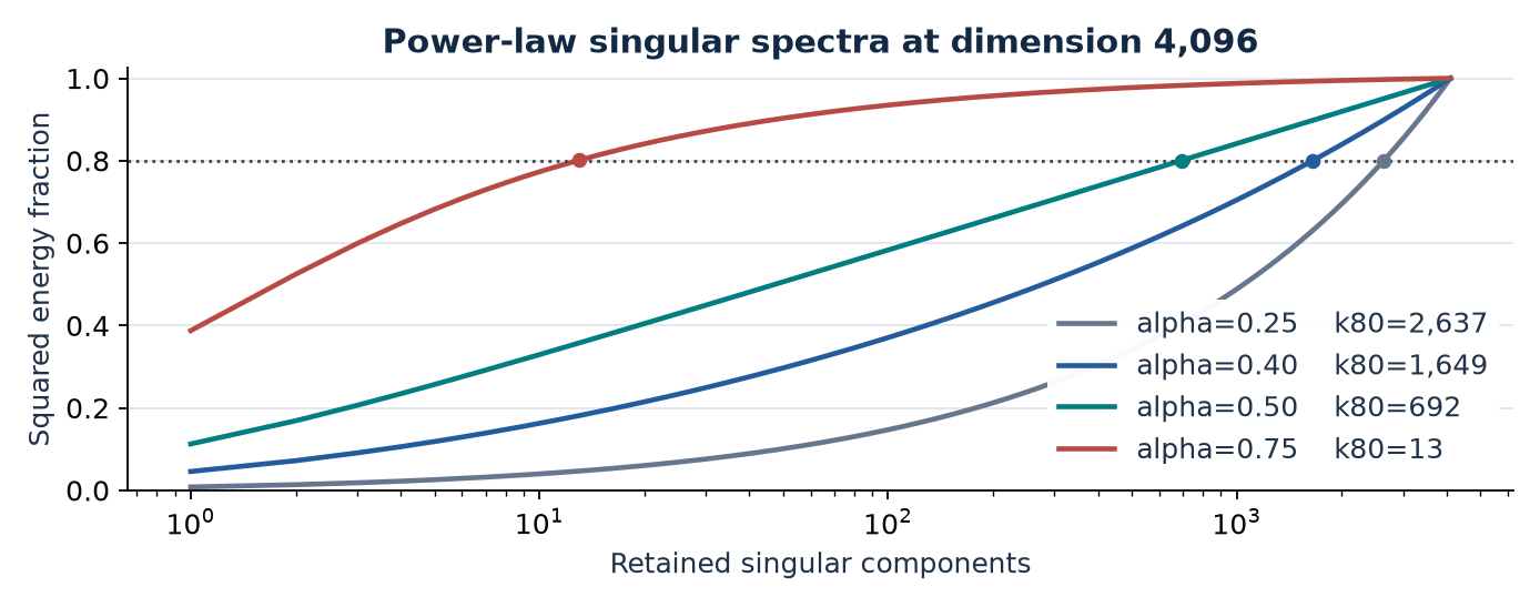
Figure 2. Original calculation at dimension 4,096 using Appendix A’s spectral construction. Dots show the first index reaching 80%. The dotted line is a fixed reporting threshold.
For , direct summation gives and . The upper bound in Eq. (4) evaluates to 22.3902 and the lower bound for to about 469.54. Appendix A prints a looser bound of 27.4 for stable rank. The important practical difference is the exact finite sum versus the one-sided lower bound on the threshold. Even the limiting ratio would suggest roughly 1,342 of 4,096 components. At this dimension, replacing by its leading-order integral loses terms that matter to a budget.
Approximate truncation and functional error
For , orthonormality makes the truncated expansion the best rank- approximation in Frobenius norm. Combining this property with the orthogonal residual gives
A threshold of 80% therefore leaves a 20% squared residual, or about 44.7% relative Frobenius norm. I keep both units explicit. A system allocating adapter storage from “80%” may interpret it as a bound on the norm or on an accuracy drop. A reconstruction threshold alone bounds neither model loss nor needed adapter training rank. The numerator and denominator describe only weight-space geometry. Even within one layer, a unit of error in a direction seldom excited by inputs can have a very different effect from the same norm of error along a common feature.
Algorithm 1. Measure the spectrum of a stage update
This is measurement pseudocode derived from paper §3.3 and Appendix E. The uniform interface accommodates both the exact calculation and a screening pass.
1  Load initial and final tensors for the same named matrix.
2  Check shape and stored orientation; widen both before subtraction.
3  Form the update and its squared Frobenius norm in FP64.
4  If the norm is zero, record a zero update with undefined ratios.
5  For a wide matrix, transpose only for spectrum measurement.
6  For a tall matrix, take reduced QR and keep the triangular factor.
7  Compute all singular values of the reduced matrix in FP64.
8  Accumulate squared values in order; divide by the Frobenius total.
9  Report stable rank, requested prefix energies and the first crossing.
10 In a screening pass, log the sketch budget and threshold uncertainty.
For a tall matrix with orthonormal columns in , the Gram matrix obeys . The singular values are square roots of the eigenvalues of this common Gram matrix, so a full SVD of preserves the spectrum. For a embedding, the QR input has about 411 million entries. FP64 storage for a dense input alone is about 3.29 GB in decimal units, whereas has 16.78 million entries or about 134 MB. QR still reads the original matrix and costs on the order of . Its benefit is reducing the shape passed to the subsequent SVD and avoiding direct eigendecomposition of an explicitly squared-condition-number Gram matrix.
A randomized method projects onto a sampled low-dimensional range. Extra columns reduce sensitivity to a hard cutoff and power iterations emphasize dominant directions. This is attractive when only a leading-value screening estimate is needed. A slowly decaying tail near the cutoff creates a harder problem: a good estimate of the maximum need not imply a good sum over 256 or 512 near-cutoff directions. An independent Frobenius total helps isolate prefix error. Using a sketched total as well can hide the energy left outside the sketch.
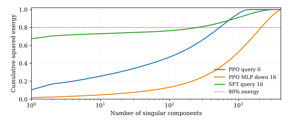
Figure 3 (paper Fig. 1). The same 80% horizontal reference gives quite different budgets for the two PPO matrices and the SFT query. The x-axis counts singular components on a log scale.
Reading the measured ranks
The paper selects seven matrix positions per endpoint by shape and layer position before inspecting approximation errors. Fourteen full decompositions offer clear existence examples. The 7B inventory contains 226 two-dimensional matrices, including 128 square attention projections, 96 MLP projections, and two large vocabulary-axis matrices. The selected cases cover query, two up projections, one down projection and the embedding. Results for key, value, output and head matrices cannot be inferred from this subset. A better sample for estimating the distribution across the model would stratify by tensor family, depth and update energy, then report the sampling weights.
| Matrix | PPO stable rank | PPO rank at 80% | SFT stable rank | SFT rank at 80% |
|---|---|---|---|---|
| Query 0 | 9.58 | 532 | 1.10 | 1 |
| Query 16 | 18.14 | 1,222 | 1.48 | 255 |
| Query 31 | 18.27 | 1,149 | 1.99 | 599 |
| MLP down 16 | 58.78 | 2,120 | 792.32 | 2,250 |
| Embedding | 1,026.35 | 2,831 | 916.65 | 2,982 |
Selected rows from paper Table 2. PPO uses the DPO reference and SFT uses the base reference. All values come from full decompositions.
Three comparisons in that table are worth separating. PPO query 16 and query 31 have similar stable ranks and threshold ranks. SFT query 0 and query 16 have stable ranks of the same order, yet their 80% budgets diverge. The two layer-16 MLP down updates have stable ranks that differ by a factor of about 13.5, but the threshold ranks are only 130 components apart. That last pair is a warning against sorting layers by stable rank before assigning ranks for a compression sweep. Appendix F also withdraws a previous PPO MLP headline near 37 because the previous reference included DPO. The correct comparison starts at the checkpoint that produced the first RLVR rollout.
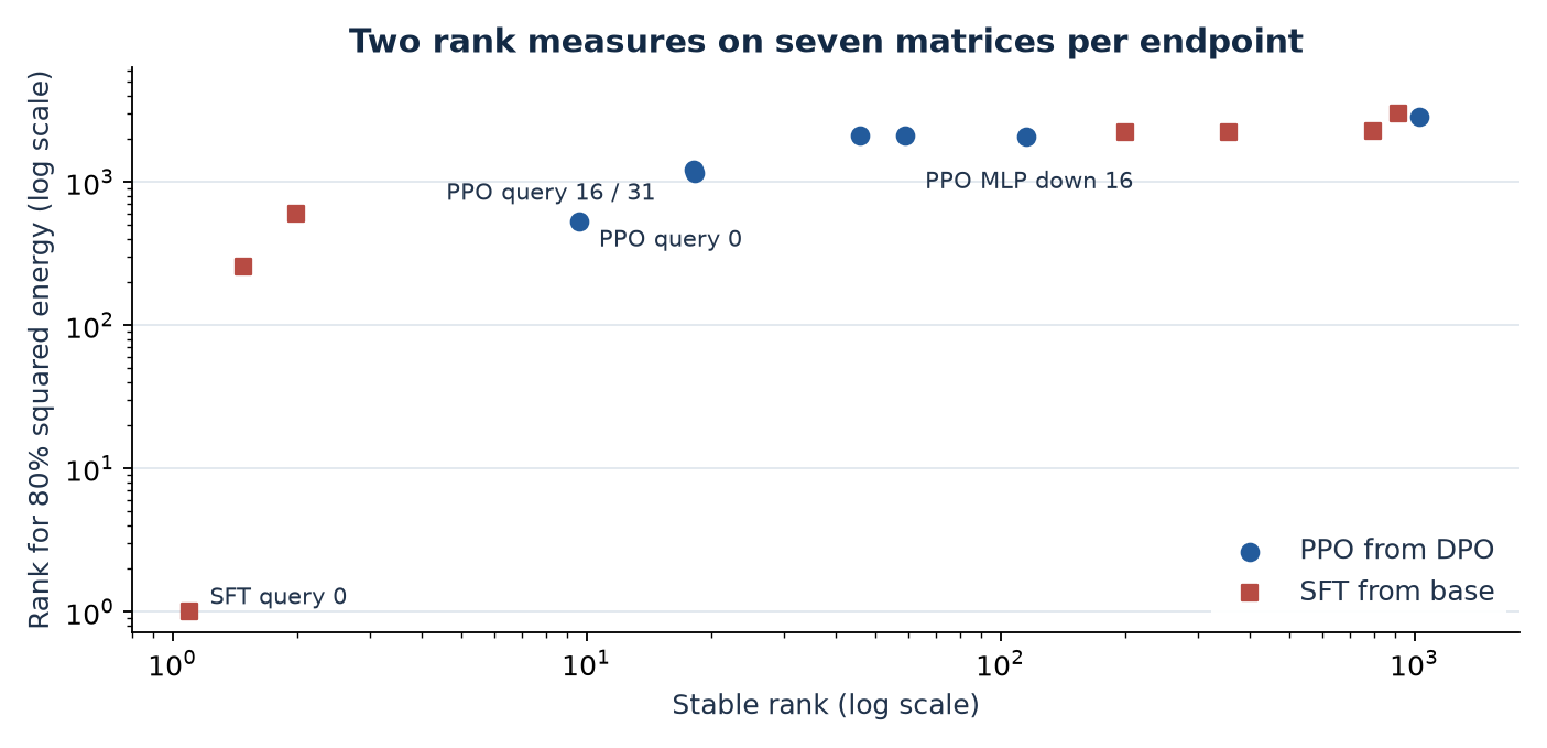
Figure 4. Redrawn from paper Table 2 with logarithmic axes. Across both endpoints, nearby stable ranks can correspond to very different truncation budgets.
A storage check turns these numbers into a concrete constraint. In a square layer, an unquantized rank- update stored as two equally precise dense factors takes about values, with singular values absorbed into one factor. Its value ratio to a dense update is . The query-zero PPO budget takes about 26% of the dense update’s value count, leaving at most 20% of the squared energy at that threshold. The layer-16 query budget takes about 60%. Both are reductions; neither translates into a serving speedup by itself. A fused dense weight can avoid a second kernel launch, and a factored update has different bandwidth and batching behavior.
Checkpoint geometry
Norms, direction and aggregation
Let be a consistently flattened model checkpoint and a finite displacement over width . For a native grid with irregular step spacing, adjacent checkpoint pairs still define displacements, but each pair must retain its own exposure units. The paper reports widths on regular grids and uses release step labels for the public models. On a fixed grid, separation picks which earlier displacement to compare to. Write the Gram matrix and use its diagonal for both norms.
Projecting the decomposition onto eliminates and gives the coefficient. Writing as cosine times the two norms gives . For the same , norm ratios 0.1 and 2 give opposing components of magnitude 2.5% and 50% of the preceding norm. The residual is perpendicular; the sum of both displacements can still be long. With and , is about , but their sum is with length about 1.22. Cosine tracks direction, and projection describes how much of the next step lies along the previous one.
Aggregation itself changes the question. If adds adjacent narrow windows into larger blocks, the Gram matrix of wider displacements is
Each block-pair dot product expands to a sum over every narrow pair across the two blocks. Averaging narrow cosines would instead normalize before summation, losing the norms and all omitted pairings. As a simple example, take positions . Native displacements alternate and so adjacent scalar cosines are . Combining two windows gives successive positive displacements of with cosine . The endpoint is shared across the two views when the grid endpoints match. This is an example of aggregation changing the sign even with a steady drift in the same direction.
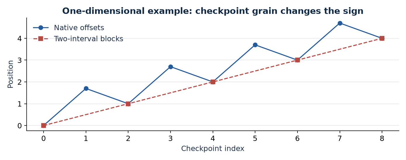
Figure 5. Original one-dimensional calculation. Saving every second checkpoint hides alternation while preserving the displacement over each two-interval block.
Algorithm 2. Accumulate the displacement Gram matrix
This measurement procedure follows the full-coordinate protocol in paper §3.3. Materializing one full concatenated vector for every checkpoint is unnecessary for the dot products.
1  Freeze checkpoint order, width, units and immediate reference.
2  Match model tensors and count each tied parameter once.
3  Initialize a square FP64 Gram matrix for all reported windows.
4  For each matched tensor, iterate blocks of coordinates.
5      Read those coordinates from each checkpoint in FP64.
6      Subtract consecutive endpoints; stack one row per window.
7      Add the block times its transpose to the Gram matrix.
8  For each lag, divide entries by the product of diagonal norms.
9  Report pair counts and mark zero-norm comparisons undefined.
10 For adjacent pairs, also report the signed projection coefficient.
A block with coordinates and windows needs temporary values. Updating a full Gram matrix over coordinates uses arithmetic and output. Computing only selected lags reduces arithmetic to for requested lags. The full matrix additionally supports reaggregation, endpoint norm checks, and comparisons of several separations without rereading every coordinate. The paper checks online and saved cosines for the six local runs to within absolute. In Appendix G, the reported in-memory versus checkpoint Gram comparison on Mistral uses more than 7.24 billion coordinates. My small generated matrix check agrees with direct multiplication to absolute and checks the chunk identity, independent of the training data.
Dependence on checkpoint storage
Suppose a saved vector differs from the underlying vector by quantization error . Then . The errors in adjacent windows share one endpoint with opposite sign. This gives a mechanism for negative observed dot products even when the latent motions are weakly aligned. I return to a variance calculation in the critical analysis. Here the protocol consequence is that FP64 subtraction preserves the available difference between saved numbers. Bits already lost at checkpoint time cannot be recovered.
The paper’s comparison of BF16 versus FP32 parameter and optimizer-state storage in Llama actually changes numerical training, including rounding along the optimization path. This differs from measuring the same latent FP32 trajectory twice after two choices of serialization. The comparison is valuable for showing configuration dependence and has limited leverage for deciding between these two mechanisms. Earlier coordinate sketch results in Appendix F are also explicitly withdrawn. A sampler that admits no coordinates after the first two million estimates the geometry of the earliest coordinates in enumeration order. Full chunked accumulation is feasible for the number of saved windows used here and removes that source of bias.
Evidence from public and supervised trajectories
Nine public stage grids
Paper Table 3 has counts of 5, 12, 12, 12, 12, 12, 16, 43 and 7, which sum to 131. All observed cosines are negative. The stage means range from for OLMoE to for OLMo-2 32B. OLMo-2 includes both PPO and GRPO, and Olmo-3 uses its own OlmoRL method label. Stage means pool different numbers of windows, so the average over all pairs would weight OLMoE’s 43 pairs more than 7B PPO’s five. Several stages share both a model lineage and intermediate checkpoints. Because adjacent pairs can share a displacement, the 131 signs should not be treated as independent Bernoulli trials.
For the public 7B PPO run, Appendix D gives five adjacent values from to . Its first-lag mean is , with four lag-two pairs averaging and three lag-three pairs averaging . The quick decline with separation is compatible with a local effect. With three distant pairs, it offers limited resolution for persistent structure at larger separations. The projection coefficients from that run range from to , so the magnitude opposing the previous direction is about 17–22% of its norm. The ratios use full parameter coordinates and describe the particular native grid.
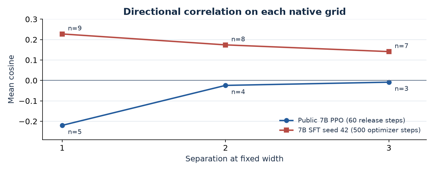
Figure 6. Redrawn from paper Table 10; counts follow Table 4. Width stays fixed within a curve. The PPO and SFT curves use different clock units.
A path-level statistic can help interpret whether many opposed steps add up to a small or a substantial displacement. Using the Gram matrix, the squared length of the total update over windows equals the sum of all diagonal entries plus twice the upper-triangular sum. In particular, negative nearest-neighbor products alone cannot determine its size. Longer-separation terms and window norms enter. I would report the endpoint norm relative to total path length along with adjacent cosines so a reader can distinguish a nearly stationary oscillation from steady drift with local corrections.
Supervised model and precision comparisons
The four-family SFT baseline runs use the same Tülu-3 mixture and 500-optimizer-step grid. They stop at 5,000 steps while retaining the two-epoch learning-rate schedule that would extend to 29,356. The longer OLMo seed-42 run supplies the spectral endpoint. OLMo and the baseline BF16 runs for Llama and Qwen have positive adjacent cosines throughout. The two BF16 Mistral runs each have seven negative pairs out of nine, beginning with the pair ending at 2,000 steps. Their full-grid means are near . The existence of these two SFT cases rules out using the sign alone to identify an RLVR stage.
The Llama follow-up retains FP32 parameters and Adam states with BF16 autocast. In the two paired seeds the full-grid means fall from approximately +0.238 to approximately +0.021. The last five pairs are negative in both FP32 runs. The first large positive windows make the full-grid average positive. Appendix G also varies the checkpoint aggregation: in FP32 Llama seed 42, the width-500 mean is +0.0206 and the width-1,000 mean is +0.0408. The width-1,500 calculation ends at 4,500 and uses two adjacent pairs. Both aggregation and endpoint coverage change in that latter comparison.
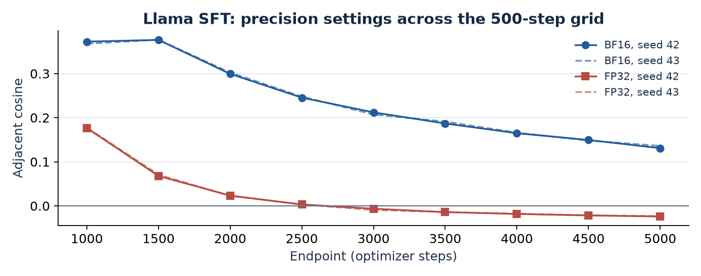
Figure 7. Redrawn from paper Table 16. The two FP32 parameter-and-state runs cross zero at the pair ending at step 3,000. BF16 and FP32 are labels for training configurations here.
The model-family comparison leaves token counts and some microbatch shapes unmatched. The follow-ups did not all precede observation of the initial result: the Mistral outcome motivated more runs and the Llama precision follow-ups. Those choices make the observed counterexamples informative and limit population-level claims. A clean follow-up would predeclare separate variations of weight storage, Adam-state storage, and forward/backward precision, with a common exposure accounting. It could also store the same trajectory under alternate checkpoint precisions at the exact same times.
The matched advantage intervention
Shared schedule and changed credit assignment
Both arms start from OLMo-2-0425-1B-DPO. Each of the three paired seeds has a shared prompt stream from RLVR-GSM. A rollout has eight prompts with eight responses each, then four passes through eight-response minibatches. There are eight minibatches in each pass. Hence a rollout advances the actor by 32 optimizer updates and produces 64 responses, and a 60-rollout geometry window corresponds to 1,920 updates and 3,840 responses. The response and prompt caps are 2,048 tokens each. Learning rate decays linearly over 360 rollout batches. The reference KL coefficient is 0.05 and ratio clipping is 0.2; actor trainable parameters and optimizer states are FP32 with BF16 autocast. A correct response receives 1, an incorrect response 0 and a missing EOS in the stated reward configuration.
Both arms reuse the actor schedule while switching the credit and normalization protocol. Group-relative training broadcasts one standardized outcome advantage per response. Critic–GAE uses a separate critic backbone and scalar head, a temporal return, tokenwise estimates, and rollout-level whitening. The critic’s value loss and optimizer add compute. Sharing prompt streams controls task sampling at the prompt level; actions, sequence lengths, KL exposure and actual generated token counts diverge. Paper Table 8 gives group versus critic token totals of 5.287M versus 5.832M at seed 42, 4.780M versus 5.861M at seed 43, and 5.072M versus 4.777M at seed 44. The contrast estimates the effect of switching the package under matched rollout and update budgets. The critic’s extra learning and changing token distribution are part of that intervention.
The independent unit is the seed pair
The primary statistic is defined on three late consecutive cosines per seed at width 60, ending at rollouts 240, 300 and 360. Average those within each run, then pair by seed. If is critic minus group at seed , the signed difference and seed-level interval are
From rounded Table 5 entries if one subtracts the displayed arm means. The table’s independently rounded last difference is . The recomputed mean from displayed arm means is , with interval approximately . With two degrees of freedom, the multiplier is about 4.303. Differences in the final decimal from Table 5 are rounding scale. Treating nine window differences as independent would shrink the standard error while counting temporal overlap as replication.
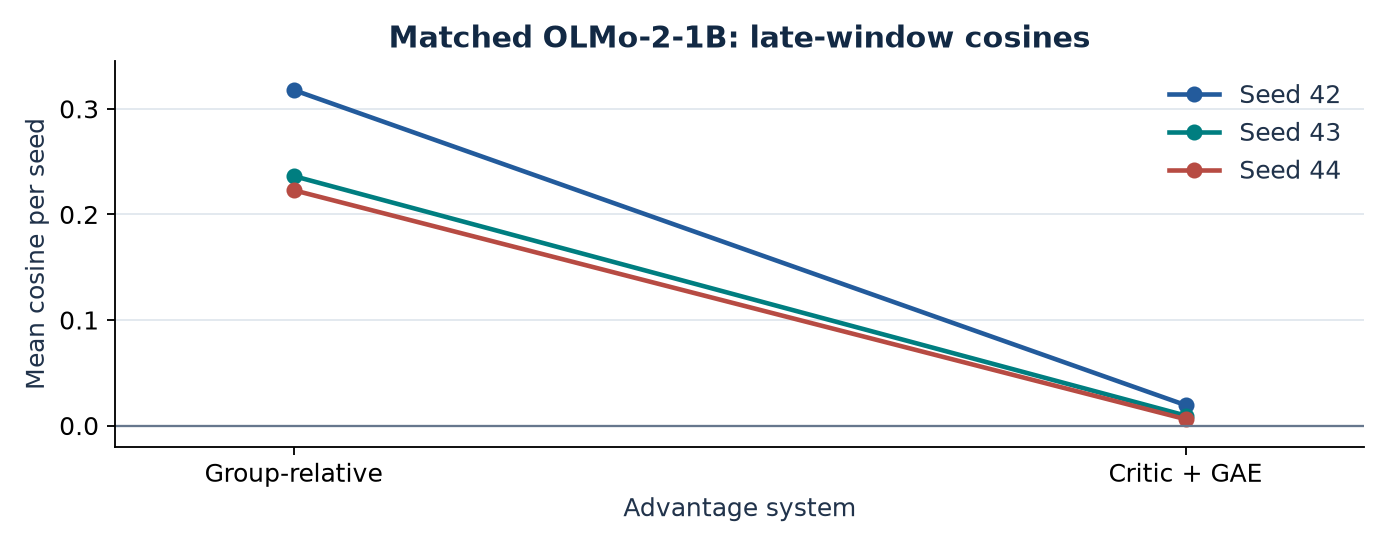
Figure 8. Redrawn from paper Table 5. A line connects runs with the same seed and shared prompt stream. The paired outcome is a decrease toward zero.
All three paired differences favor lower alignment in the critic arm. The critic arm’s own mean is about +0.012 and its interval includes zero. Thus the controlled result describes a shift toward zero. All observed public stages have considerably negative adjacent means, including public GRPO. The two controlled arms did not reproduce that public sign pattern. Widths 10, 20 and 40 support the direction of the contrast descriptively. Their intervals use the same seeds and overlapping checkpoints; the paper does not adjust for multiple comparisons across widths. For width 40, eligibility is determined by the endpoint label, so one included window crosses the midpoint.
This study has six runs but three paired statistical units. A distribution-free sign test illustrates how little information that contains about a population median. Under exchangeable independent signs and a continuous null centered at zero, three differences all having the same sign gives probability for the two-sided extremity. The Student interval uses distances and modeling assumptions in addition to signs. The two summaries answer differently specified questions. I would keep the raw three seed differences visible alongside the interval, and repeat the paired intervention with more seeds before using the magnitude to select a production algorithm.
Training health and scope
The fixed 32-example greedy diagnostic starts at 20 correct and ends between 16 and 20 across the six runs. Group-relative runs give 32 EOS completions each on that diagnostic, whereas the critic arm gives 27, 28 and 29. Training cap-hit rates are lower in the critic runs, so lower cap-hit during sampling and lower EOS completion in the greedy diagnostic coexist. They are different measures on different datasets and protocols. Appendix B reports finite-update checks and a correction from earlier truncated response-cap experiments. Neither the paired interval nor the health counts establishes an improvement in task quality. A larger held-out set, explicit reporting of truncated and invalid samples, and return distributions by prompt difficulty would make the geometry easier to connect to behavior.
Numerical validation and measurement choices
An unresolved threshold has two possible explanations
The paper’s rank-256 stress case is the SFT layer-16 query update. Full decomposition gives and . With a common FP64 denominator, three baseline sketch seeds give 0.79754418, 0.79760081 and 0.79759122. The stronger sketch gives 0.79972833. Thus the full prefix exceeds the target by about 0.02792 percentage points while the stronger estimate falls below it by about 0.02717 points. A deterministic assertion that the true rank exceeds 256 would be false for this matrix. Across the fourteen cases, the paper finds a maximum error of about 1.353 percentage points at rank 512. Stable rank with the accurate denominator has at most about 0.0088% relative error in the baseline comparison. The original normalization increases its worst error to 2.38%.
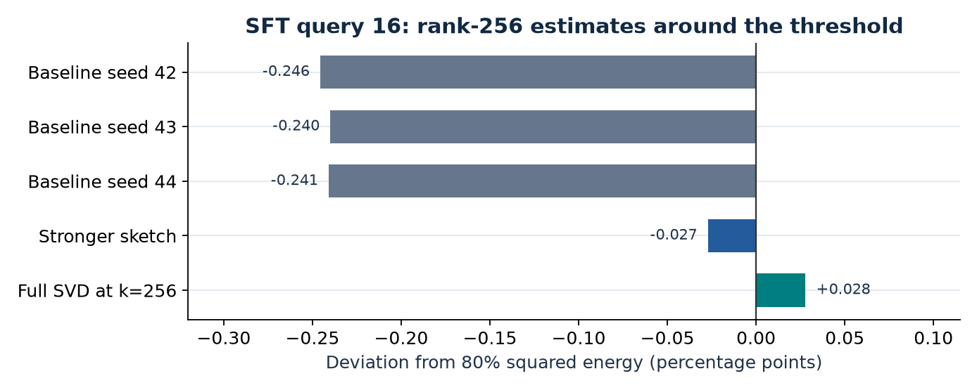
Figure 9. Redrawn from Appendix E. All bars use the same denominator and the rank-256 budget. The full prefix just clears the threshold; its first crossing occurs at rank 255.
If the solver certifies an interval , then certifies sufficiency and certifies insufficiency. If the interval straddles , report the budget as unresolved. One way to get a one-sided bound uses an orthonormal trial space . Projecting to restricts the admissible left vectors for a rank- approximation, so the leading squared singular energy of is a lower bound. This can certify that a budget suffices in exact arithmetic when normalized by the full energy. A simple complementary upper bound adds the projection residual energy to the lower bound. Write and . For any matrix with orthonormal columns, . Maximizing over , the first term is at most the squared top- sum of , and the second at most .
The residual bound can be loose for a broad tail. In floating point the orthogonality and norm estimates must carry adequate margins. Stronger range finding or a complete decomposition narrows the interval. This triage criterion is my extension of the paper’s reporting policy and requires validation before replacing its exact calculation.
Weight-subspace angles measure a different matrix pair
Appendix E compares the leading 64 left singular vectors of the weights before and after training. This is independent of applying SVD to the weight difference. For equal-dimensional orthonormal bases , the smallest singular value of is the cosine of the largest principal angle. The residual projection gives its sine. To see this, reduce its self-product using idempotence of the projector.
At a tiny angle , is about . At this difference is about , below ordinary FP32 spacing near one. Computing the small residual with orthonormal FP64 bases avoids asking an arccosine to resolve that difference from a rounded number near one. The paper’s original calculation uses both randomized bases and FP32 arccos, so the difference between it and the new calculation is a combined change. In the PPO embedding the values are and . The largest absolute discrepancy in Table 13 comes from SFT MLP up at layer 31, about . A large spectral gap at rank 64 can support a stable basis estimate, whereas a cluster straddling the cutoff can make the largest angle depend on small numerical perturbations. I would record each boundary gap with the angle, particularly if a subsequent method uses those subspaces as a fixed constraint.
Measurement checklist for a follow-up
A paper-faithful comparison starts with a manifest of checkpoint labels, the immediately preceding checkpoint, tensor orientation, dtype, and the exposure unit. For each model list which weights are tied and which vectors enter the full measure. To compare SFT and RLVR keep objective details, mask, initialization, optimizer, precision, schedule and training horizon alongside the figures. This lets a reader explain an apparent contradiction without assuming it is a mistake. Appendix F documents why the initial PPO reference is DPO and why old claims from the limited sketch and unmatched experiments were withdrawn.
For the spectral record I would carry dimensionality, absolute update norm, norm ratio to the reference, leading value, stable rank, energies at several explicit rank budgets and exact threshold rank or a sensitivity interval. Record approximation settings and whether the trace was normalized against total energy. Run deterministic small checks first: diagonal ground truth, an orthogonal change of basis, an all-zero case, and a tall matrix whose direct spectrum agrees with its reduced QR spectrum. The local random-matrix QR check in this review gave identical singular values at displayed precision. A high-aspect-ratio embedding test can then exercise memory and timing independently of end-task evaluation.
For direction I would retain the Gram matrix, displacement norms, every pair’s window labels and the final cosine and projection readings. A known two-window example should match both vector arithmetic and block computation. A wider grid should use a stated offset and exactly the endpoint coverage requested by the comparison. For the intervention, report seed-level means, per-seed differences, token and optimizer exposure, the cap-hit rates and end-task uncertainty on a larger diagnostic. The paper reports its public inventory in Appendix D and local protocol in Appendix B. The counts provide useful checks even when a larger study will eventually change the schedule.
Limitations
The theorem establishes possibility under a specified power law. There is no fit in the paper showing that each selected spectrum obeys that law over all directions. Stable rank and threshold rank are scale invariant, so the difference between a barely moving matrix and a strongly changed matrix disappears unless its absolute norm is also reported. Fourteen matrices cannot map the variation over all 226 matrices of one model, much less across architectures. The two 7B endpoints also start from different checkpoints and have different training histories. The numerical results establish where the gap occurs in the selected sample.
The survey covers OLMo releases on the grids at which checkpoints are available. Native widths vary, release step labels differ in exposure, and stages share lineages. Measured signs are robust descriptions of those saved sequences. Generalization to other methods, model families or timescales requires additional trajectories. The SFT counterexamples show that negative cosines can arise under a supervised objective. The precision follow-up changes several numerical properties, including optimizer-state precision. The matched intervention isolates the advantage package under its own actor schedule. It changes a fitted critic, temporal credit, whitening population and realized token counts together. Three seeds in one 1B setting and a 32-example task diagnostic provide limited statistical and behavioral resolution.
Critical analysis
Test whether the error can account for the lag profile
An adjacent pair shares one subtraction endpoint. With independent, zero-mean storage errors across checkpoints and independent of every true displacement, the expected additional adjacent dot product is negative. Expand the product of the error differences. Three of four terms vanish by independence; the shared term remains with a minus sign.
The same idealized mechanism contributes nothing in expectation at lag two or higher because no endpoints are shared. This calculation concerns dot products, with cosine denominators also affected. Quantization errors are generally neither independent nor independent of the trajectory. The derivation is a diagnostic for designing measurements, not an estimate of the paper’s bias. The near-zero lag-two and lag-three means in the public PPO example make the alternative testable. Measure exactly the same higher-precision checkpoints before and after controlled rounding, compare lag profiles on both, and stratify by update-to-roundoff ratio. Include resampling or staggered checkpoint grids at several widths to separate one-endpoint artifacts from genuine dynamics that decay over time.
Test compression on activations and task outcomes
I would separate two uses of low rank. The first approximates an already-trained full update. The second trains inside the family of low-rank factors and may find a different endpoint. For the first use, the Frobenius criterion assumes all input directions count equally. If is the layer input with second moment , and , linear output distortion expands as
A broad tail can be inexpensive to remove on one prompt distribution and consequential on another. Conversely, a small tail aligned with frequently activated features can produce disproportionately large output distortion. A credible ablation should allocate equal total factor storage across recipes and compare magnitude-based, fixed-energy and activation-weighted truncations on both training-like and shifted prompts. Keep per-layer absolute norms and compare output error, verifier pass rate, calibration and deployment cost. Then train LoRA at a few matched budgets from the same immediate reference. An experimentally successful low-rank path would answer a different question from the best Frobenius approximation of a full update. The paper supplies a useful pretest for estimating where these approaches could disagree.
Separate correction, noise, and credit assignment
The paired study changes a package. A follow-up can vary the learned baseline and whitening population separately while retaining terminal rewards, prompt pools and actor schedule. Compare group-relative, a leave-one-out prompt baseline, a state-value baseline with full-return advantages, and GAE at multiple trace decays. Run both an on-policy paired protocol, which estimates the effect of the training regime including subsequent behavior, and a frozen-rollout comparison, which asks how much the immediate gradient direction changes on identical token sequences. Record raw gradients, preconditioned updates and checkpoint displacement cosines as distinct quantities. Observing which stage of the pipeline introduces anti-alignment would narrow the plausible mechanism.
I would also split global dot products by tensor family. The global numerator is a sum of block inner products, while normalization uses global norms. Averaging the cosines of layers would change the estimand because it gives a low-energy layer equal weight. Reporting signed block contributions and their shares of each displacement’s energy would show whether a handful of tensors dominate. Combined with the same checkpoint grids and the storage-precision experiment, this gives a way to assess whether attention, embeddings or the MLP are driving a geometric effect. The existing full-coordinate measurements make this a natural extension of the analysis.
Conclusion
The paper’s cleanest lesson is about choosing the quantity before estimating it. The leading singular value determines how stable rank is normalized. A cumulative threshold asks how far the tail must be traversed for a chosen residual. The Gram matrix asks whether finite moves on a stated grid point together, and the paired intervention shows how much that reading changed under one credit-assignment package. I would use full-SVD energy or certified bounds when allocating irreversible compression budgets, report multiple widths and actual norms when interpreting displacement cosines, and test any claimed effect on quality on the task itself.
References
- Khalil and Hoque. Spectral Rank and Step-Direction Dynamics in Language-Model Post-Training, v1. Methods in §§2–3, results in Tables 2–5, numerical and protocol details in Appendices A–G.
- Hu et al. LoRA: Low-Rank Adaptation of Large Language Models.
- Schulman et al. High-Dimensional Continuous Control Using Generalized Advantage Estimation and Proximal Policy Optimization Algorithms.
- Halko, Martinsson and Tropp. Finding Structure with Randomness.