Silent Instrument Errors | What an agent leaderboard actually measures

Review date: 2026-11-09
Author: Zhongzhu Zhou
Paper reviewed: Silent Instrument Errors Reorder Agent Leaderboards
Paper author: Yangze Liu
arXiv: 2611.04399, version v1, 2026-11-03

1. Four ways to get a plausible wrong number

An airline agent changes a flight reservation and sends a closing message. The new reservation is already in the database. The simulator, however, does not emit the token that marks the interaction done, and the scaffold exits before another step. In the archive the episode has reward zero. On a leaderboard that zero looks just like a checked reservation that failed the task. An evaluator which scores the database at a declared boundary could assign a different outcome to the same interaction.

Yangze Liu studies this kind of disagreement in two public evaluation systems, the Holistic Agent Leaderboard (HAL) and $\tau^2$-bench. Three HAL cases concern the execution that produced the original record. The fourth concerns how $\tau^2$-bench reads and re-grades old records. The paper’s comparison is unusually useful because the agent interactions are fixed. The author changes the measurement or re-derives it from lower-level evidence, without generating a new rollout.

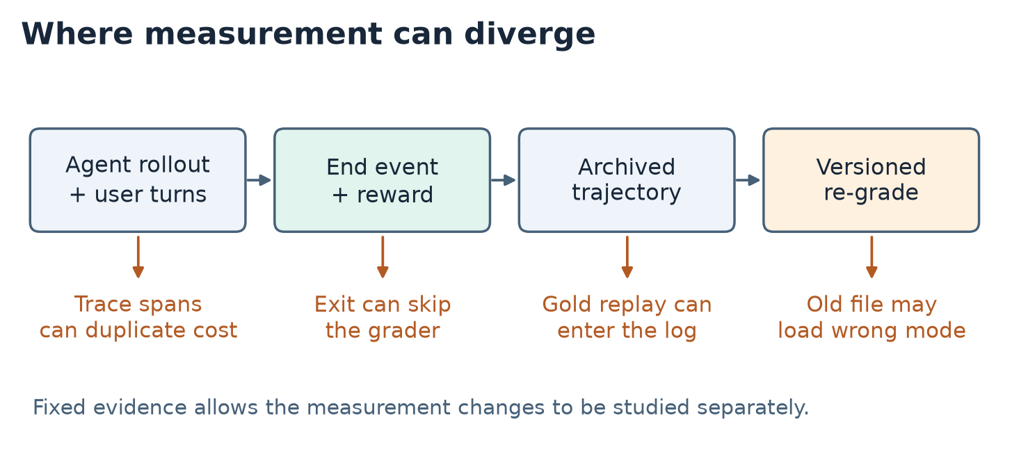
Figure 1. Original schematic from paper §§2–3. The arrows follow the evidence from the live interaction through grading and archival to re-grading. Cost runs alongside this path because its evidence is the trace tree.

My reading separates four objects. The task rule describes success. The termination policy decides when to evaluate it. The trace schema describes which events happened and who produced them. The leaderboard aggregates scored episodes and cost. A change to any one can move a published number. A change to the task rule may be intentional and improve validity, while a wrong environment mode during replay can produce an invalid measurement under the very same rule. The banking and telecom cases illustrate that distinction particularly well.

The most consequential HAL result is specific. For nine shared models on a subset of 41 airline tasks, the Generalist scaffold’s pooled score moves from 0.30 to 0.43 when every episode is graded, closing a 13-point published gap with the Tool-Calling scaffold. On write-required tasks the Generalist moves from 0.28 to 0.33. These are reported archive results. Below I reconstruct their logic, derive sensitivity bounds and check arithmetic from the paper’s tables. The bounds and toy examples are my analysis.

2. Prerequisites

State, episodes and evaluator boundaries

A tool-using agent alternates between messages and actions. Let $x_0$ be the initial environment state, $a_t$ an executed action and $o_t$ its returned observation. With the simulator and tools fixed, a replay transition can be written as

$$(x_{t+1},o_t)=F_e(x_t,a_t), \qquad x_T=F_e^{(x)}(\cdots F_e^{(x)}(x_0,a_0),\ldots,a_{T-1}).$$

Here $F_e^{(x)}$ denotes the state component of the transition and $e$ includes the environment and its mode. A trajectory is more than this sequence of states. It can include messages, tool responses, actor identities and a termination event. A textual answer can matter to the reward independently of the database. For the cases here it is helpful to imagine a reward $R_v(x_T,m,g)$ that receives the terminal state, relevant messages $m$ and task criteria $g$ under evaluator version $v$. This is an abstraction for the reading. The paper applies the benchmark’s own reward.

There can be three distinct boundaries. The scaffold has stopped requesting model completions. The environment has received a terminating event. The grader has emitted an outcome. Some systems make all three coincide. In HAL’s airline case a tool transferring to a human or a stop token from the simulated user can trigger grading, while the Generalist can finish its loop by sending a closing turn. A monitor which only counts explicit system errors will miss a missing outcome if the pipeline serializes it as a number.

Measurement coverage and units of comparison

A rollout can be scored as a pass or a fail, remain ungraded, or be unreadable for re-grading. The intended denominator may be all planned episodes, all launched episodes, or only successfully scored episodes. Each answers a different question. For an interactive benchmark, stopping in an unusable state can itself be a failure, while losing a score after successfully completing a task is a measurement problem. An explicit reason code permits both distinctions.

Repeated runs of the same model and scaffold on a fixed task are also different from independent tasks. Pooling episode counts weights models with more archived runs more heavily. Averaging model-level rates gives each model equal weight. In a matched task analysis the same task belongs to both scaffolds, which makes shared difficulty a useful control. A paper can show a clear direction of correction with data too sparse to settle each individual scaffold ordering. I keep the pooled, per-model and per-run claims separate below.

Trace trees and effective invoices

A tracing span records an operation and often contains parent and child identifiers, timestamps and a payload. A scaffold wrapper can start a span, call a provider client with its own span, and record the same response on both. Token usage belongs to the provider response or billable attempt. An aggregate over spans is valid only when its selected events are a partition of the billable work. If the wrapper and the child both report it, their usage fields overlap. Request retries matter because two different charged attempts can have identical arguments. An identity-based accounting rule needs an identifier for the billable event and a pricing convention.

Why reproducibility has two layers

Given an archive, the first question is whether it carries sufficient evidence about the original interaction. Given that evidence, the next question is whether an evaluator can reconstruct the relevant environment and faithfully apply the intended criteria. Reproducing the published scalar under the original evaluator answers a fidelity question. Scoring a fixed interaction under a new rule answers a version comparison question. If the rule and the replay environment both change, the scalar alone cannot identify the source of a change.

3. When the grader never runs

Deriving the gap contributed by missing grades

Let $G_i$ indicate a triggered grade and $Y_i$ be the binary score that would result from a faithful evaluation of episode $i$ under the declared target rule. For a fixed set of $N$ episodes, the stored zero convention gives

$$\begin{aligned} S_{\mathrm{stored}}&=\frac{1}{N}\sum_i G_iY_i =f\,\bar Y_g,\qquad f=\frac{1}{N}\sum_i G_i,\\ S_{\mathrm{all}}&=\frac{1}{N}\sum_i Y_i =f\,\bar Y_g+(1-f)\bar Y_u,\\ S_{\mathrm{all}}-S_{\mathrm{stored}}&=(1-f)\bar Y_u . \end{aligned}$$

The second line splits the sum into the graded and ungraded strata, with means $\bar Y_g$ and $\bar Y_u$ when their strata exist. The difference assumes the observed grades stay fixed and a target score is defined for every episode. The missing outcomes contribute the last term. No independence assumption is needed for this identity. It would be needed to fill in $\bar Y_u$ by reusing $\bar Y_g$. In this case the grading trigger depends on how the scaffold ends the episode, so such an imputation would conflate behavior and selection.

For two scaffolds $A,B$, subtracting their identities gives

$$\Delta_{\mathrm{all}} =\Delta_{\mathrm{stored}} +(1-f_A)\bar Y_{u,A} -(1-f_B)\bar Y_{u,B}.$$

A small difference in execution quality can be hidden by a large difference in the probability of being measured. As an illustrative example, suppose both systems solve 44 of 100 tasks under the target rule. System A has 50 scored episodes, with 30 passes. System B has 98 scored episodes, with 43 passes. Their stored scores differ by 13 points. The correction adds 14 and 1 points respectively, so both land at 44%. This example uses one cohort for all denominators. I do not divide the paper’s pooled 13-point gain by $1-0.51$. The quoted 51% is a graded fraction over the episodes discussed in §3.2, while the reported pooled score uses the selected non-terminal-gold task subset and shared-model comparison.

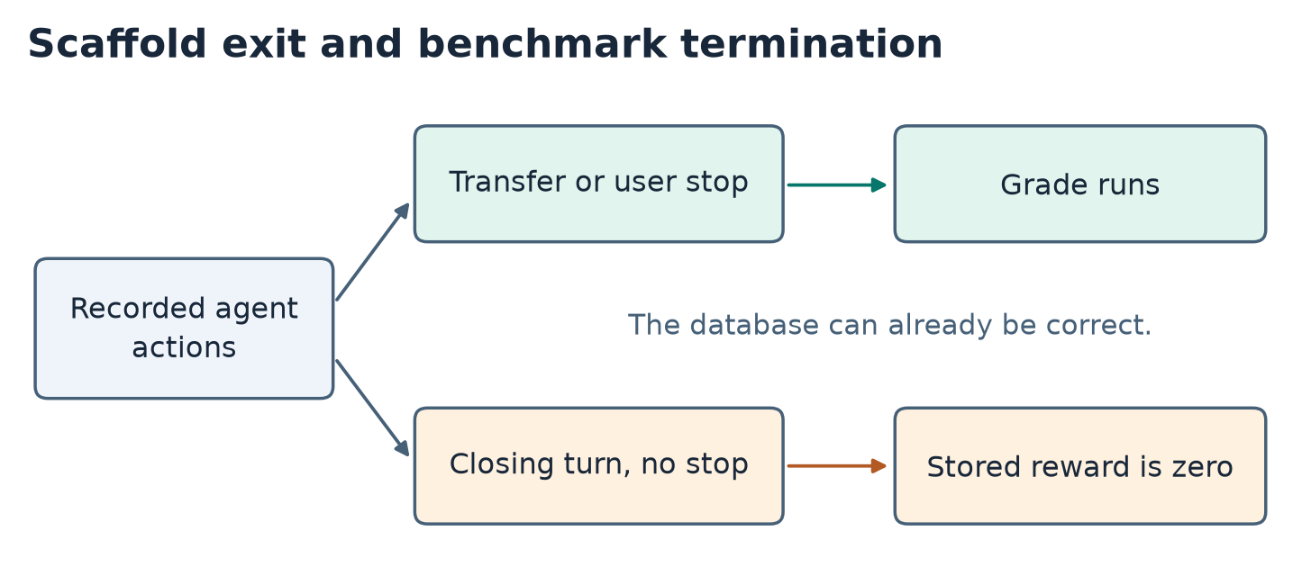
Figure 2. Original schematic from paper §3.2. The two exits can occur after equivalent database actions. A close message only yields a grade if it leads to the benchmark’s ending event.

Algorithm 1. Recover grades using the actor’s trace

This numbered pseudocode summarizes the method described in §§3.2–3.3 and Appendix A. The ending-event check is a validation on records with known outcomes. The replay for the missing stratum uses the environment and reward under the paper’s specified constraints.

01 Group records by task, model, scaffold and run.
02 Parse executed agent tool calls from the raw model log.
03 Match the calls in order to archived actions by name and arguments.
04 Locate unmatched reference actions anywhere in the archived list.
05 Mark graded if a reference replay is detected or reward is positive.
06 For known grades, check recorded endings and replay agreement.
07 Keep the observed grade for each already graded record.
08 For an ungraded record, start at the task's initial state.
09 Replay agent actions with user and model calls stubbed.
10 Apply the benchmark database and output checks.
11 Record source of grade, write requirement and replay diagnostics.
12 Pool within the same task filter and compare with stored outcomes.

A reference sequence at the end was the author’s initial signature. Appendix A corrects it by searching throughout the record. A Generalist transfer can trigger the grader before a later closing turn, so a suffix-only rule missed 73 Generalist episodes whose injected copy sat inside the record. The positive-reward condition in line 05 also covers a grade whose reference replay has no identifiable extra actions. A zero without a recognizable gold replay remains harder to classify, especially when the task has an empty or trivial gold action list.

The method avoids regenerating conversations and preserves the recorded policy decisions. A full fresh run would exercise termination again, but the simulated user and model could take different paths, breaking the fixed-evidence comparison. Grading the last archived state directly would avoid replay if trustworthy snapshots were saved. If tools have side effects absent from the archive, or a user response depends on those effects, replay can diverge. Those cases motivate a reported replay-validity denominator alongside the corrected score.

4. Cost belongs to the billable event

Deriving the duplication multiplier

Let $\mathcal B$ be the set of uniquely charged events in a run. Let $c_b$ be the cost of event $b$ under one fixed pricing policy, and let $k_b$ count its copies in usage-bearing spans. With exact copies the intended and observed totals obey

$$\begin{aligned} C_*&=\sum_{b\in\mathcal B} c_b,\qquad C_{\mathrm{all}}=\sum_{b\in\mathcal B} k_b c_b,\\ \frac{C_{\mathrm{all}}}{C_*} &=1+\sum_{b\in\mathcal B} \frac{c_b}{C_*}(k_b-1). \end{aligned}$$

Each additional copy adds its own cost to the numerator. The ratio is therefore a cost-weighted mean multiplicity, for $C_*>0$. If every call appears twice, the ratio is two even with a mixed pricing schedule. If only expensive calls are duplicated, the ratio can be far greater than the fraction of spans that are duplicates. The same identity holds for a consistent token usage metric after substituting token counts for cost. Different input, output and cache prices mean that a token multiplier need not equal a dollar multiplier in a heterogeneous run.

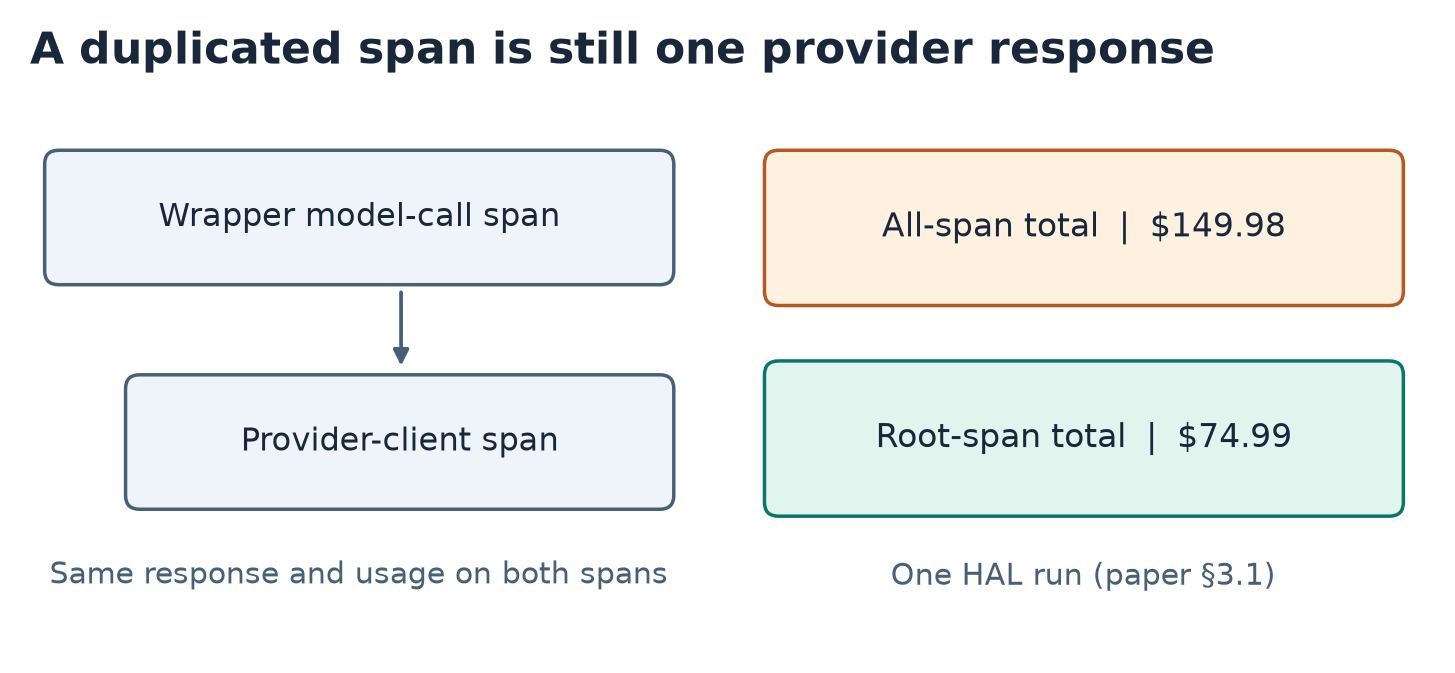
Figure 3. Original trace schematic and a paired example from paper §3.1. The archived $149.98 and root-span$74.99 are for one Tool-Calling Claude Opus 4.1 high-reasoning airline run.

Algorithm 2. Diagnose cost inflation at run granularity

This is a reading of §3.1 and Appendix A with the reporting safeguards from §5. The primary reconciliation operates on the run, which is the unit at which the published total was formed.

01 Read the reported usage and the model-call trace tree for a run.
02 Exclude runs without a usable usage block from ratio estimates.
03 Sum usage over all model-call spans with measured payloads.
04 Sum again over root model-call spans in the same trace.
05 Compare all-span usage to the archived aggregate.
06 Align nested spans by provider response and usage when possible.
07 Compute cost using the same prices and compare both totals.
08 Report both counts, their ratio and unresolved trace coverage.
09 Compare ratios across benchmark, scaffold and provider path.
10 Recompute cost-accuracy dominance only on comparable cohorts.

The root-span approach is appropriate in the case described because the outer model-call span carries the response and duplicates the child. An orchestration span can instead contain several independent billable child calls and have no aggregate usage. Choosing global trace roots would then drop those charges. An event-ID alternative needs namespace and attempt semantics to avoid dropping two legitimate provider charges under one logical request ID. A double check with provider billing records would separate span duplication from stale prices and from missing usage. One diagnostic ratio cannot guarantee complete accounting.

Appendix A says reported usage equals the all-call sum in 133 of 134 runs with logs. Table 1 reports exactly doubled tokens in 70 of the 134 and unity in 46. The cost comparison reports 36.5% excess over root-span cost across 133 runs with usage, and §3.1 separately reports 44 doubled costs among 94 matchable leaderboard rows. These counts describe different units. Appendix A counts 138 decrypted archives across three named benchmarks and mentions additional archives used for the cost analysis. I would not use it as the denominator for the matched-row statistic.

A frontier can change even with identical accuracy

Call row $i$ dominated when some row $j$ has score $S_j\ge S_i$, cost $C_j\le C_i$, and at least one strict inequality. If all cost values are multiplied by one positive constant, every inequality on costs survives. Row-specific multipliers can reverse them. For illustration, take A at 0.58 accuracy and 40 dollars, and B at 0.56 and 60 dollars. A dominates B at correct prices. If only A has doubled cost, its displayed cost becomes 80 dollars and both appear on the frontier. The accuracy column is unchanged. On SciCode the paper reports a scaffold-dependent pattern with all ten zero-shot runs clean while many other runs have nearly doubled cost. The toy dominance calculation explains the direction of the risk without inferring which particular SciCode points cross the frontier.

5. A trajectory can contain somebody else’s actions

Reference replay and causal attribution

To compare a final state against the gold target, a grader can replay reference actions from a clean initial state. Reusing the environment transition is sensible because the same tool semantics should apply. In the airline case the transition also writes into a shared action list. Once the archiver stores that list under the agent’s record, the grader’s write history can be mistaken for the agent’s.

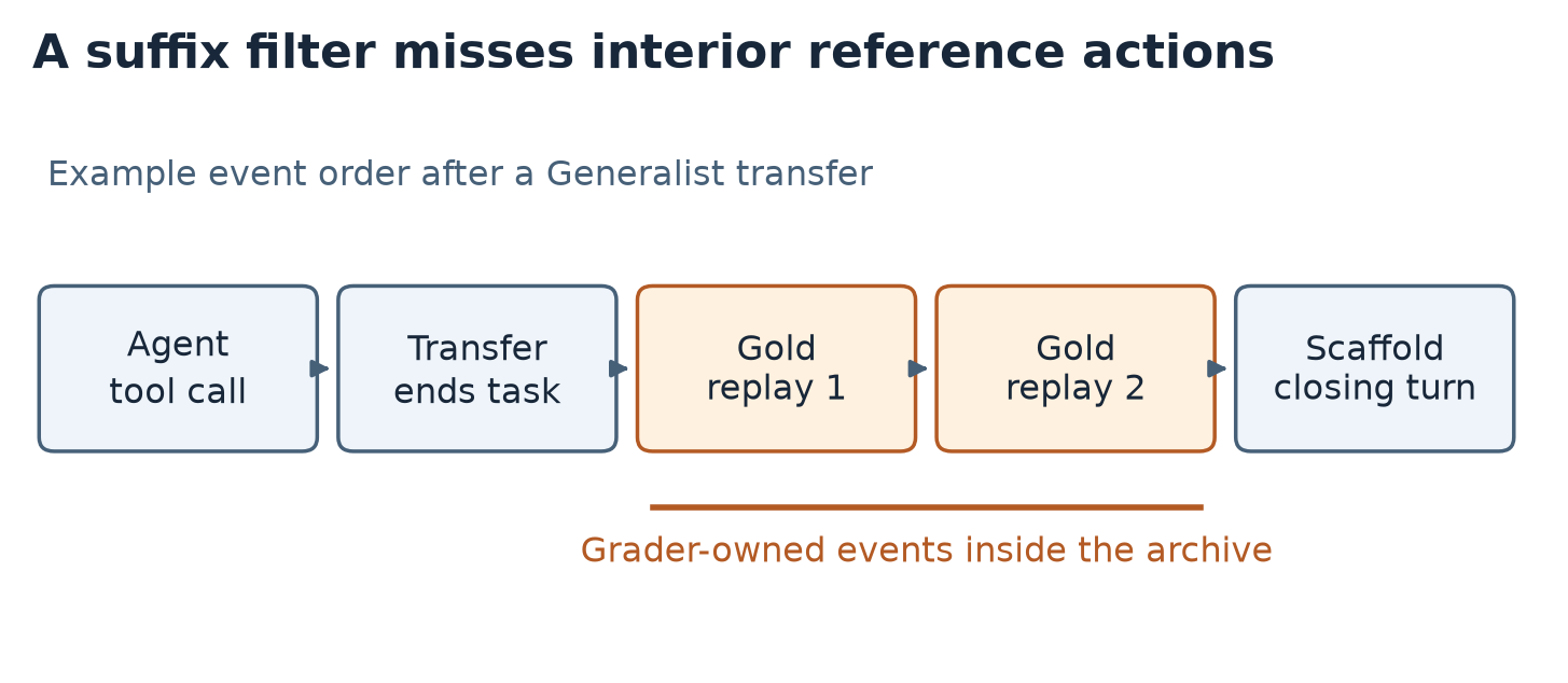
Figure 4. Original timeline from paper §3.3 and Appendix A. A Generalist transfer can precede a reference replay and a later scaffold closing message, leaving grader actions inside the archived sequence.

Write the logged sequence $L$ as an interleaving of agent actions $A$ and reference replay actions $H$, omitting other actors for this derivation. If provenance were known, a simple projection would recover $A$:

$$L=(\ell_1,\ldots,\ell_n), \qquad A=(\ell_j:\operatorname{actor}(\ell_j)=\mathrm{agent}).$$

Without actor labels, the paper aligns the ordered actions from the raw model trace to the archived list. The alignment uses tool name and arguments. It finds an order-preserving map $\phi$ such that

$$\phi(1)<\cdots<\phi(|A|),\qquad \operatorname{key}(a_i)=\operatorname{key}(\ell_{\phi(i)}).$$

The unmatched actions are candidates for grader provenance in the paper’s record design. A valid alignment is not generally unique. For example, if an agent reads reservation 42 and the gold replay repeats that exact read, a list with two identical actions allows two assignments. For a later error analysis the difference matters when the two copies have different positions or responses. A monotone match is more informative than deleting the last $|H|$ items, but the clean long-term design is to attach provenance before serialization.

Algorithm 3. Preserve evidence when a reference is generated

This is a prospective design derived from paper §5, rather than a claim that the released benchmark used it. Immutable events let the original sequence and the reference construction coexist.

01 Assign stable episode, event, actor and replay identifiers.
02 Execute agent tool calls against the live episode environment.
03 Append the inputs and observed results to the live event stream.
04 At the declared boundary, snapshot the live terminal state.
05 Start an isolated reference environment from the task initial state.
06 Replay gold in the reference stream using its own event identifiers.
07 Compute reward from live evidence and the isolated reference.
08 Store grade, validity and provenance without rewriting live events.
09 Verify the live event stream hash before exporting the record.

An alternative is a shared event stream with separate actor and execution-phase fields. It can preserve ordering across the grader and the live episode, but still needs separate mutable state so a reference action cannot change the state being evaluated. Separating the environment alone is insufficient if both contexts share an event sink. In a distributed run, event IDs should include namespace and attempt so retries do not overwrite the original evidence.

Paper §3.3 finds injected actions in 68% of 2,334 public airline records and reports 58 records that show a complete gold tool sequence although the agent made no tool call. In the subset whose gold contains at least two non-terminal actions, verbatim replay reproduces the recorded reward in 70% of records. Removing injected actions raises agreement to 92%. That 22-point gain is a consistency check on the trajectory interpretation. It does not measure a 22-point improvement in the agent.

6. Re-grading fixed trajectories with changing instruments

Cross evaluator and task data

For a saved trajectory $i$, let $v$ be the evaluator build, $g$ the task-data revision and $e$ the reconstructed environment mode. Write the replay score as $s_i(v,g,e)$ when replay is valid. Take the mean over the same parseable files and same episodes to define $S(v,g,e)$. With mode held fixed, the change between an old and a new combination can be decomposed by adding and subtracting a crossed cell:

$$\begin{aligned} S(v_1,g_1)-S(v_0,g_0) ={}&[S(v_1,g_0)-S(v_0,g_0)]\\ &+[S(v_1,g_1)-S(v_1,g_0)]. \end{aligned}$$

The first contrast holds task data fixed at the old version. The second holds code fixed at the new version. Swapping the order of the contrasts gives another decomposition. Their difference in attribution is the interaction

$$I=S(v_1,g_1)-S(v_1,g_0)-S(v_0,g_1)+S(v_0,g_0).$$

If $I$ is nonzero, an additive explanation tied to one order is incomplete. A crossed cell may be impossible when an old evaluator cannot parse a new task revision. The comparable cohort and invalid cells should remain visible. Mode is a separate intervention because it determines which tool calls are available and which state changes can be reconstructed.

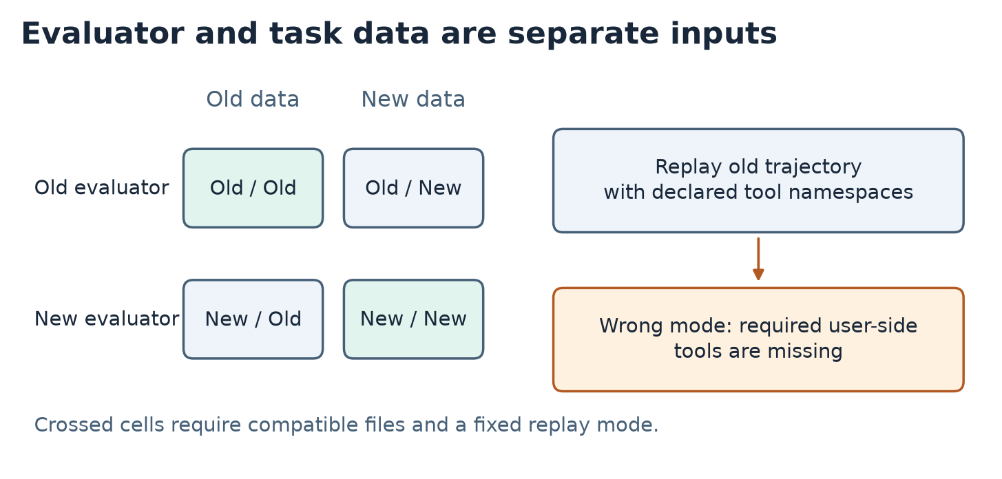
Figure 5. Original schematic based on paper §3.4 and Appendix A. Crossed cells keep the saved behavior fixed while varying evaluator and task data. A wrong environment mode breaks replay before reward is applied.

Algorithm 4. Compare versions with a replay gate

Lines 01–05 describe the paper’s crossed comparison at a high level. Lines 06–09 include checks I would add to a leaderboard instrument, informed by the paper’s recommendations.

01 Select archived trajectories and record task and evaluator revisions.
02 Identify the declared replay mode and required tool namespaces.
03 Choose old and new evaluator and task-data combinations.
04 Run each compatible combination on the same saved trajectories.
05 Record every per-episode outcome under each combination.
06 Compare recorded versus replayed tool results and state checkpoints.
07 Mark invalid replay separately when a required capability is absent.
08 Publish valid counts, score changes and pass/fail transitions.
09 Count rank reversals and ties on a common declared cohort.

Using a strict replay gate protects against a score from an invalid environment. It can also exclude archives with benign response-format changes. A more targeted gate separates schema mismatches from state-changing tool failures and compares normalized result fields under documented rules. With a missing user-side tool in a dual-control task, a warning is too weak because the replay state is structurally incapable of applying the recorded action. A mode inferred from a display name is brittle. A schema field for the mode and a capability check at load time would make this failure visible before replay.

7. What the archived results establish

Airline scaffold comparison

The paper reports grader coverage of 51% for Generalist and 98% for Tool-Calling. The Generalist’s ungraded trajectories end in a message at a median of nine actions, well below a step cap. In the pooled nine-model comparison on tasks with non-terminal gold actions, its published 0.30 rises to 0.43 after scoring the missing episodes. Tool-Calling changes by at most 2.5 points in any shared-model row. A large part of the pooled gain comes from tasks with read-only gold actions, for which an unchanged database can satisfy the database criterion. On the tasks that require a write, the Generalist moves from 0.28 to 0.33. The paper reports 23 newly passing ungraded episodes with the necessary write in the agent’s own calls. This slice makes the strongest case that an infrastructure decision hid successful actions. It still inherits the benchmark’s output and state criteria.

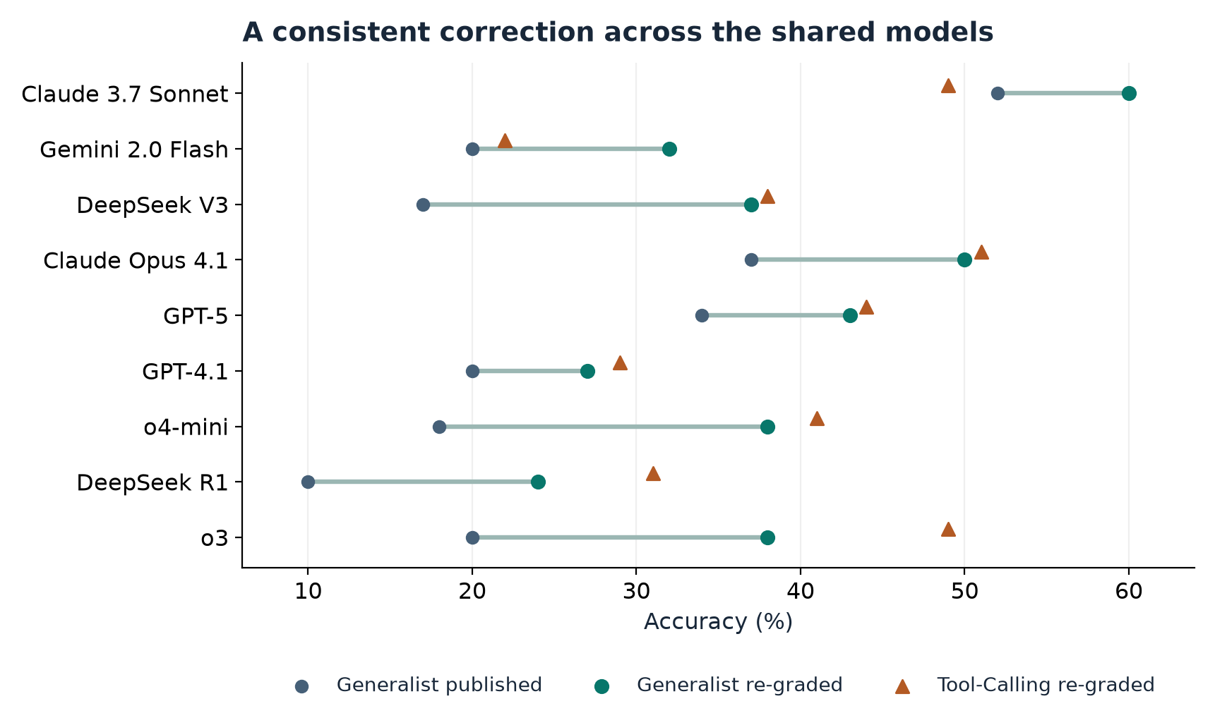
Figure 6. Redrawn from paper Table 2 for the nine models with both scaffolds. Tool-Calling markers are after re-grading. The Generalist sample is 40–82 episodes per model. The graph shows rounded rates and omits the withdrawn Few-Shot scaffold.

The movement toward parity is consistent across models. The paper reports eight of nine Generalist rows behind as published and seven after grading all episodes. Gemini 2.0 Flash changes order: Table 2 gives 0.20 and 0.32 for Generalist, around the 0.22 Tool-Calling comparator. Claude 3.7 Sonnet was already ahead under the original grades. DeepSeek V3 closes from 0.17 to 0.37 against 0.38. Read those rounded rates with the underlying counts. One trial in a cell of 41 moves the rate by about 2.44 points. One or two runs of the same task set also share task difficulty. A small final gap cannot be interpreted as a stable model-specific advantage.

The fidelity checks in Appendix A use two different replays. Re-running the grader at recorded ending events with gold embedded in the records reproduces all 1,951 recorded grades. Replaying only the agent’s own actions on graded episodes matches 97% of Tool-Calling, 97% of Few-Shot and 84% of Generalist grades. The latter is closer to the procedure applied to ungraded episodes. Most Generalist disagreements in that check change an original pass to an offline failure. The author interprets this as evidence that the correction may understate the Generalist. I would treat the direction as suggestive on the ungraded set because the two groups need not share the same missing state or ending behavior. The paper also checks alternative gold definitions on the three tasks that differ between the fork and the pinned task set and reports no change to the pooled result.

Banking, airline and telecom measure different changes

The banking update in $\tau^2$-bench 1.0.1 announced that older scores were incomparable. In the paired files the author attributes score movement to evaluator code, with no observed pass-to-fail transitions. Yet Gemini 3 Flash moves from ninth to tied fifth on the official before-and-after leaderboard. A policy that allows only upward per-episode moves does not preserve the relative order of models: their improvements can differ.

In the airline update the task criteria for 14 of 50 tasks changed substantively while the database and policy remained fixed. Applying the new criteria to four older files changes 77 of 800 simulation outcomes, in both directions. That is $77/800=9.625\%$ of the outcomes. Model-level score changes range from minus seven to plus 2.5 percentage points. A single net difference can hide two large opposing flows. With pass-to-fail count $n_{10}$ and fail-to-pass count $n_{01}$ on $N$ matched outcomes, the net and the fraction that changed are

$$S_{\mathrm{new}}-S_{\mathrm{old}}=\frac{n_{01}-n_{10}}{N}, \qquad F_{\mathrm{flip}}=\frac{n_{01}+n_{10}}{N}.$$

The first identity subtracts away episodes that kept their original grade. The second keeps both directions. A balanced pair of flows can give no net movement while changing which tasks a model appears to solve.

In telecom, four solo files were interpreted with the wrong mode and replay lacked user tools. Lenient replay continued after failed calls. The reported losses are 59–82 points, and a companion file with the recognized solo mode returns its recorded score. This is a negative control for the mode explanation. It concerns how the saved interaction is reconstructed, whereas the banking result concerns how a faithfully replayed interaction is evaluated.

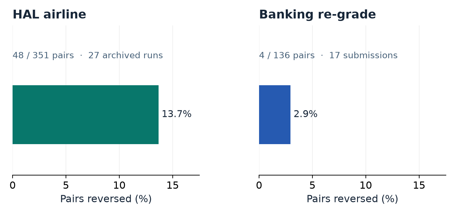
Figure 7. Redrawn from paper §§3.2 and 3.4. The denominators are 351 pairs of 27 HAL runs and 136 pairs of 17 banking submissions. Rates are arithmetic from the reported counts, with each panel referring to its own cohort.

For $n$ units the unordered pair count is $n(n-1)/2$. If $d^0_{ij}$ and $d^1_{ij}$ are old and new score differences, strict reversal requires opposite signs, $d^0_{ij}d^1_{ij}<0$. Ties can be published separately. The paper reports 48 of 351 reversed HAL run pairs, about 13.7%, and four of 136 banking submission pairs, about 2.9%. These are descriptive fractions. Pairs share units and do not provide 351 or 136 independent Bernoulli trials. A leaderboard should document tie tolerance, especially when displayed scores have fewer digits than the scoring data.

8. Limitations

Two leaderboards, with three cases sharing the HAL airline stack or its infrastructure, are evidence that these failure mechanisms occur in practice. They give no sampling frame for the frequency of such errors across the field. The paper explains why the architecture admits them. Estimating prevalence would require choosing benchmarks and versions independently of whether a failure had already been suspected.

The HAL correction evaluates a pinned replay with a stubbed user and model. Its estimand is the database and output reward on those saved interactions under the prescribed rule. A cooperative user might have supplied a missing answer on another turn, or a live user might have rejected a technically valid state change. The study holds behavior fixed. The result should travel with the cohort filter and reward definition.

The corrected comparison is between existing scaffolds as built. They differ in step budgets and in how the airline policy is exposed. The author notes that Tool-Calling includes the policy in its system prompt while Generalist has to open a file. Equal grading removes one source of distortion. It does not separate the causal effects of policy access, interaction style and scaffold generality. The withdrawn Few-Shot results include a known leakage issue and serve as context in Appendix A.

The analysis reports agreement and score changes on available archives. A frozen archive can omit inputs or lose provenance in ways that rule out faithful replay. The observed public records can also be selected, such as the five banking leaderboard files parseable under all compared builds. The 17-submission reversals use the official before-and-after table, a different evidence set. I read each result within its denominator.

9. Critical analysis

Coverage should bound a claim before it is corrected

From §3, because $0\le\bar Y_u\le1$, the original record alone gives a worst-case interval

$$S_{\mathrm{stored}}\le S_{\mathrm{all}} \le S_{\mathrm{stored}}+1-f.$$

Subtract the upper endpoint of B from the lower endpoint of A for the smallest plausible gap, then subtract B’s lower from A’s upper for the largest. That yields

$$\Delta_{\mathrm{stored}}-(1-f_B) \le \Delta_{\mathrm{all}} \le \Delta_{\mathrm{stored}}+(1-f_A).$$

These are identification bounds under the fixed observed-grade assumption, not confidence intervals. They remain wide when coverage is low. If replay recovers some missing episodes with trustworthy grades, the bounds shrink by moving their outcomes into the observed stratum. If replay validity is unknown, moving them into that stratum creates false precision. I would report three denominators on each affected cell: planned episodes, graded episodes, and valid recovered episodes. The coverage and replay gate then determine which comparisons can be made without strong assumptions.

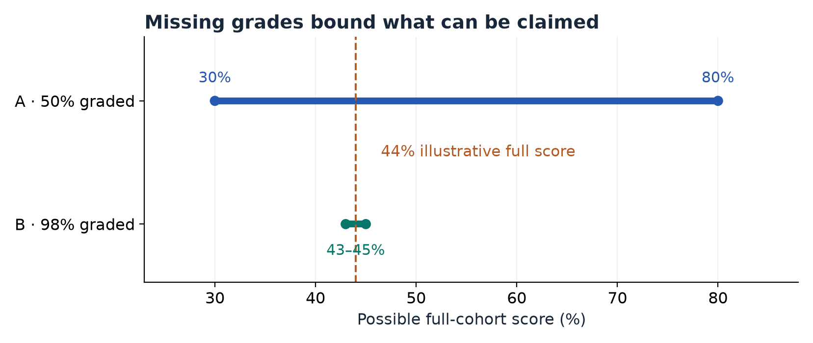
Figure 8. Illustrative calculation using the 100-episode example in §3 of this review. A stored 30% with 50% coverage allows 30–80%, while a stored 43% with 98% coverage allows 43–45%. The common 44% point is the hypothetical full-cohort score.

Replay agreement needs its own stratification

I would strengthen Appendix A with a per-task table that crosses termination reason, task write requirement, model, scaffold, and replay validity. In particular, the 84% agreement on graded Generalist records merits inspection of which disagreements require a simulator observation that was not archived. If mismatches concentrate in particular tools, the re-grade could mark the corresponding ungraded episodes unresolved and report lower and upper bounds after partial recovery. If they concentrate only at a distinct type of termination, that makes the direction of the correction more credible. A prospective experiment could save terminal-state digests and force scoring at a scaffold-independent boundary, then compare original-grade and replay-grade outcomes on the same fresh episodes.

I would also publish two contrasts for read-only tasks. One uses the original rule and one adds an explicit correctness check for the requested information. On a task that asks for the fare class, leaving the database untouched tells us little about whether the answer is correct. The original rule is appropriate for isolating an instrument error. The stricter rule asks whether the underlying metric captures service quality. A large shift in one contrast and a small shift in the other would be a substantive result. Treating all read-only corrections as useful service would hide that distinction.

A sensitivity analysis for the unresolved episodes

The widest missing-grade bounds treat any outcome as possible. If only some missing grades can be recovered, a sensitivity analysis can show what would have to be true for the ordering to change. Suppose scaffold $j$ has $N_j$ original episodes, $P_j$ original or recovered verified passes and $U_j$ episodes still unresolved. Let $q_j$ be the unknown pass fraction of those episodes. The score compatible with a choice of $q_j$ is

$$S_j(q_j)=\frac{P_j}{N_j}+\frac{U_j}{N_j}q_j.$$

The slope is the unresolved fraction. Equal values of $q_A$ and $q_B$ need not be a neutral assumption when unresolved fractions differ. For $U_A>0$, setting $S_A(q_A)=S_B(q_B)$ and moving the verified rates to the right gives the tie threshold

$$q_A^*(q_B)= \frac{N_A}{U_A} \left(\frac{P_B}{N_B}-\frac{P_A}{N_A} +\frac{U_B}{N_B}q_B\right).$$

If the threshold is outside $[0,1]$, a tie is impossible for that value of $q_B$. If it is inside, the ordering can depend on the unresolved cases. In the toy cohort from §3, before any recovery, $P_A=30$ and $U_A=50$, while $P_B=43$ and $U_B=2$. The threshold is $0.26+0.04q_B$. A tie at $q_B=0.5$ requires $q_A=0.28$, consistent with the example’s 14 missing passes for A. I would publish thresholds by task class rather than borrow a single pass propensity from successful replays. A state-changing tool failure can make the unresolved cases systematically harder to recover than an absent closing event.

A second sensitivity check concerns pooling. On a common set of task-model strata $h$ with weights $w_h\ge0$ summing to one, form

$$\Delta_w=\sum_h w_h(S_{A,h}-S_{B,h}).$$

Changing from episode weighting to equal-model weighting changes $w_h$ and can move the pooled comparison even after grading is consistent. Using one weight vector for both scaffolds removes a difference in cohort composition. It requires support on both sides. If an archived stratum has only one scaffold, keep it in a separate coverage table instead of silently treating the absent side as a failed task. In this paper the Table 2 Claude Opus 4 row is an example: it has Generalist results and no Tool-Calling comparator. I would ask a leaderboard to report the matched and all-available aggregates side by side with the included tasks and weights.

Rank reports need paired uncertainty and an audit trail

Reversal counts make the consequences concrete, but rankings compress correlated estimates into an order. I would pair the same task and matched model wherever available, then resample tasks as blocks while retaining both scaffolds’ observations. If repeated runs are plentiful, add a second level for run-to-run variation. Report the distribution of the paired gap, along with the number of tasks and trials it uses. This is a proposal for future analysis. It does not replace the archive’s descriptive correction. For a decision about which scaffold to deploy, an equivalence margin on pass rate and a price range are often more informative than ordering cells with a one-episode difference.

An immutable score row can reference the evidence bundle, task revision, evaluator build, pricing and grading boundary, with separate outcomes for success, failure, ungraded and invalid replay. On correction the old row can remain reproducible and link to a new row and a diff. The erratum should ship with downloaded records, not just the website. A small set of fixtures can test that equivalent end states get equivalent grades, injected reference actions cannot enter the live event stream, and retries billed twice remain distinct. The boundary fixtures matter more than proving one particular runtime path correct.

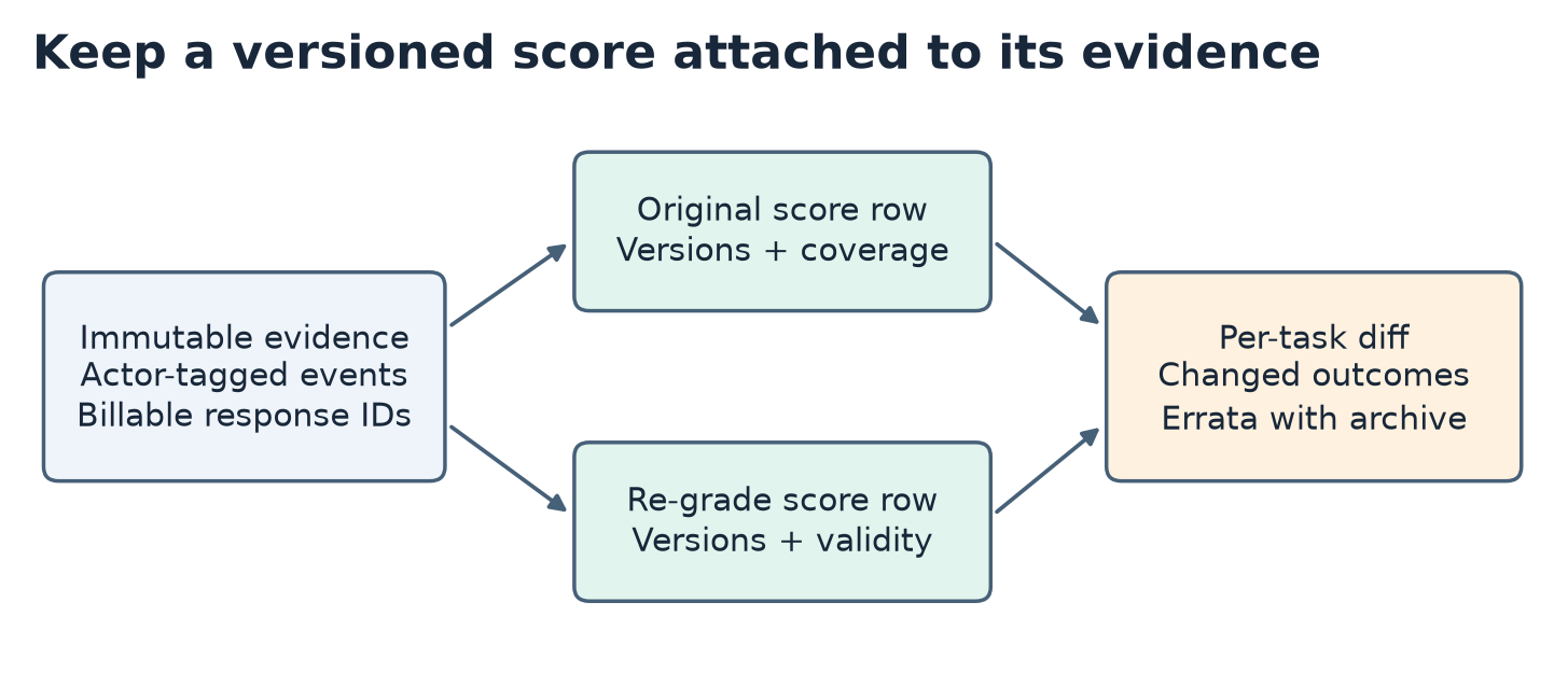
Figure 9. Proposed score-row record based on paper §5. A rerun of the evaluator emits a new result linked to the same fixed evidence and a per-task diff. Keeping coverage and validity fields visible makes regressions easier to locate.

10. Reproducibility and conclusion

The best reproducibility evidence in the paper is a set of comparisons on fixed public records. To interpret them I would preserve the 41-task filter for the pooled HAL claim, use the Appendix A grading rule that detects interior gold actions, and keep the original observed grades when correcting the ungraded stratum. For the cost case I would record the pricing convention and compare matched run IDs at all-span and root-call levels. For the version case I would preserve the original file, evaluator/task versions, mode, comparable cohort and per-task outcomes. The banking fidelity target in Appendix A is 0.2474 for Claude Opus 4.5 under 1.0.1 against the official 24.74%. That check is distinct from comparing score changes across 17 submissions.

This reading reproduces the arithmetic and draws the figures from the cited values. It does not claim a new agent run or an independent re-grade. For reuse, the author links a disclosure and artifact resource. The HAL archive discussion provides the public disclosure and correction history, including the maintainers’ confirmation. The HAL paper, $\tau$-bench and $\tau^2$-bench define the evaluation systems. Rollout Cards and the agent log analysis study give related approaches to preserving and interpreting rollout evidence.

I would read a leaderboard score as a claim about a specific run under a particular measurement configuration. When that claim includes the graded fraction, billable-event convention, action provenance and replay validity, a change can be traced to its cause. The HAL correction shows how the apparent cost of using a general scaffold can shrink once the benchmark measures its episodes. The banking comparison shows that a documented evaluator improvement can still change a leaderboard ordering. Together they make the evidence behind each score part of the result.