HarnessBandit: Which Agent Interface Should Receive the Next RL Update?

Review date: 2026-11-03 · Author: Zhongzhu Zhou
Paper: HarnessBandit: Joint Learnability-Transferability Scheduling for Multi-Harness Agentic Reinforcement Learning
Paper authors: Hongliang Wei, Xiaobing Tu, Yinggui Wang, Zhengxi Liu, Rongkun Xue, Jinkui Ren, Xiantao Zhang, Debin Zhao, Xiaopeng Fan
arXiv: 2609.13739 · Version: v1, 2026-09-12

1. The decision is which interface should produce the next training batch

A language model does not interact with a software workspace by itself. A harness chooses a system prompt, exposes tools, translates model output into actions, and manages the conversation. The same model and task can therefore produce different trajectories under OpenClaw and Codex. Training through several such interfaces is attractive because deployment interfaces change. It also creates an allocation problem: which interface deserves the next expensive batch of agent rollouts?

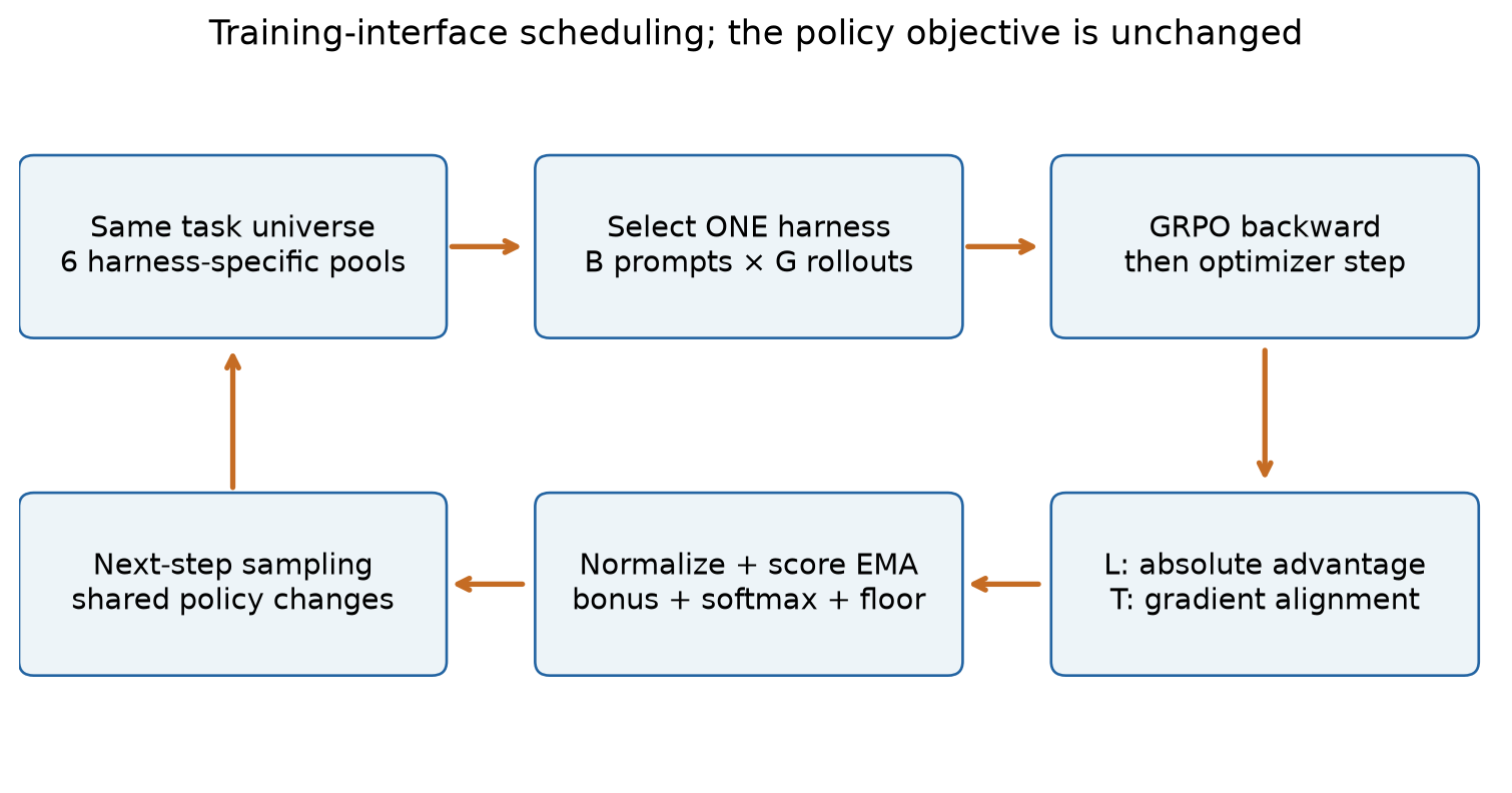
HarnessBandit gives this decision to a small online scheduler. Every optimizer step uses a batch from exactly one harness. After that batch has supplied advantages and a gradient, the scheduler records two signals: the magnitude of the group-relative advantages and the alignment of a compact gradient representation with past gradients from the other harnesses. It combines the signals, updates a running score, and changes the distribution used to choose subsequent harnesses. The shared policy still receives an ordinary GRPO-style update.

The useful distinction is between an interface that offers a learning opportunity and an interface whose update may transfer. A harness that produces both successful and unsuccessful attempts supplies a reward contrast. But that contrast might teach tool syntax specific to that interface. Conversely, a direction that resembles other harnesses’ gradients may be unhelpful if it arises from an already solved batch or mostly reflects a shared regularizer. Combining the signals is a plausible heuristic for balancing these concerns; it is not a direct measurement of future evaluation reward.

The reported Qwen3.5-2B experiment improves the PinchBench mean from 0.493 for an OpenClaw–Codex mixture to 0.506. On ClawEval, HarnessBandit solves 67 of 161 tasks at least once in three attempts, compared with 62 for a six-harness mixture. However, its 43 tasks solved in all three attempts merely match the untuned base model’s count. The method improves some dimensions of adaptation without establishing a general reliability improvement or a wall-clock training speedup.

This review uses the complete 13-page paper, including Appendices A–F. Reported measurements below are taken from its tables. All analytical examples, reconstructed figures and proposed experiments are explicitly separated from those measurements. In particular, two numerical ambiguities in the appendix deserve clarification rather than silent correction.

2. Prerequisites: tasks, harnesses, groups and gradients

2.1 A harness changes the trajectory distribution

Let $x$ denote a task, including the user request and initial workspace. Let $h$ denote an execution interface. A rollout is a sequence of model tokens, tool actions and observations, which I denote by $z$. The checker assigns a terminal reward $r(z)\in[0,1]$. Even if the initial task is identical, the distribution $\pi_\theta(z\mid x,h)$ depends on the harness: different tool descriptions and error feedback change which actions the policy attempts and what it observes afterward.

This is different from assigning mathematics to one arm and coding to another. HarnessBandit crosses the same 2,000 ClawGym tasks with six interfaces, producing 12,000 task–harness rows. The arms are Gemini CLI, OpenCode, Qwen Code, Pi, OpenClaw and Codex. Each arm maintains a shuffled pool of the same task universe. This controls the gross difference in task support between arms, although the particular tasks visited at a particular moment still differ.

A shared task universe does not make the arms interchangeable. One harness may be better at presenting a file tree; another may require a more brittle tool-call format. The scheduler could be learning which interface currently exposes useful tasks, which produces easier execution, or which gives gradients compatible with the others. These mechanisms can coexist. A single overall reward curve cannot distinguish them.

2.2 Why a group of attempts is useful for RL

For a selected prompt, the trainer samples $G$ trajectories. A baseline removes the part of the reward common to the group. The paper describes a leave-one-out baseline without division by the reward standard deviation. Writing the reward of attempt $i$ as $r_i$, the elementary estimator is

$$A_i=r_i-\frac{1}{G-1}\sum_{j\ne i}r_j =\frac{G}{G-1}(r_i-\bar r), \qquad \bar r=\frac{1}{G}\sum_i r_i. \tag{1}$$

The second equality follows by substituting $\sum_{j\ne i}r_j=G\bar r-r_i$. Positive advantages increase the relative probability of successful actions; negative advantages discourage worse attempts. A group in which all rewards are identical has no reward contrast, even when every attempt succeeds. Thus average reward and training usefulness need not rank groups in the same order.

The distinction also explains why the signal must be interpreted alongside filtering. The reported setup removes groups with zero reward variance through dynamic sampling. The training batch is consequently selected from groups that survived a reward-dependent filter. A mean calculated on survivors describes those survivors, not the entire rollout distribution and not the cost of finding them.

2.3 What remains unchanged in the policy update

Using $\rho$ for a current-to-rollout policy probability ratio and $\delta$ for the clipping radius, the loss has the familiar form

$$\mathcal L(\theta)= \mathbb E\!\left[-\min\!\left( \rho A,\operatorname{clip}(\rho,1-\delta,1+\delta)A \right)\right] +\lambda_{\rm KL}D_{\rm KL}(\pi_\theta\Vert\pi_{\rm ref}). \tag{2}$$

Here $\delta$ is deliberately different from the scheduler’s exploration parameter. HarnessBandit chooses the data source for this loss. It does not project conflicting gradients away, add a new task reward, or train six independent policy models. The reference policy is frozen; the policy being optimized is shared across all arms.

The gradient used as a transfer observation is obtained after accumulation over the selected batch and before the optimizer update. This timing matters. A partial microbatch gradient would be a noisier and potentially biased representation of the selected arm. A gradient measured after changing parameters would refer to a different policy. Observations arrive only after paying for a selected arm’s rollout and backward pass; the scheduler does not inspect every arm’s current gradient before choosing.

3. Learnability: a useful contrast, with an important conditioning effect

3.1 The hierarchy of averages

The paper first averages absolute token advantages over each trajectory’s valid token mask. It then averages trajectories within a prompt group and averages groups within the selected harness. If $M_i$ is a trajectory’s token mask, the hierarchy is

$$\ell_i=\frac{\sum_t M_{i,t}|A_{i,t}|}{\sum_t M_{i,t}}, \qquad L_h=\frac{1}{|\mathcal G_h|} \sum_{g\in\mathcal G_h}\frac{1}{|g|}\sum_{i\in g}\ell_i. \tag{3}$$

This construction gives each group equal influence. A long attempt does not dominate the scheduler simply by containing more generated tokens. That is a sensible choice when the scheduling unit is a task group. It is not necessarily the same weighting used by every term of the optimization loss, so $L_h$ should not be read as the norm of the policy gradient.

Large absolute advantage indicates substantial reward contrast. It says little by itself about gradient variance, clipping saturation, rollout latency, or the relevance of the contrast to deployment. The scalar deliberately discards direction. A useful scheduler needs either another signal or a strong assumption connecting local contrast to downstream improvement.

3.2 Deriving the binary-reward case

Consider an explanatory special case: rewards are either zero or one, and $k$ of the $G$ attempts succeed. Equation 1 gives

$$A_{\rm success}=\frac{G-k}{G-1}, \qquad A_{\rm failure}=-\frac{k}{G-1}. \tag{4}$$

There are $k$ successful attempts and $G-k$ failures. Averaging their absolute advantages therefore yields

$$L(k)=\frac{1}{G} \left[k\frac{G-k}{G-1}+(G-k)\frac{k}{G-1}\right] =\frac{2k(G-k)}{G(G-1)}. \tag{5}$$

For $G=8$, the maximum occurs at $k=4$ and equals $4/7$, approximately 0.5714. Both a completely failed group and a completely solved group receive zero. A scheduler maximizing this quantity alone tends to prefer intermediate difficulty, but intermediate difficulty is defined relative to the current model, harness and reward checker.

The same upper bound applies to the mean absolute leave-one-out advantage for eight rewards anywhere in $[0,1]$. One way to see this is that the mean absolute deviation is convex in the reward vector. A maximum over the unit cube can be attained at an extreme point, which reduces the problem to binary rewards and Equation 5. This observation will matter when interpreting the appendix’s raw signal plot.

3.3 Filtering changes what the scheduler sees

Suppose, only for this analytical example, that the $G$ attempts independently succeed with probability $p$. Because $k$ is binomial, $\mathbb E[k(G-k)]=G(G-1)p(1-p)$, giving

$$\mathbb E[L]=2p(1-p). \tag{6}$$

A nonzero-variance filter keeps a group unless all attempts fail or all succeed. Its retention probability is

$$P_{\rm keep}=1-(1-p)^G-p^G. \tag{7}$$

The discarded groups have $L=0$. Dividing the unconditional expectation by the retention probability therefore gives

$$\mathbb E[L\mid\mathrm{keep}] =\frac{2p(1-p)}{1-(1-p)^G-p^G}. \tag{8}$$

At $p=0.1$ and $G=8$, only about 56.95% of groups survive, but their expected learnability is about 0.316. At $p=0.5$, nearly every group survives and the conditional mean is about 0.504. The filtered signal compresses the distinction between rare useful groups and abundant useful groups. Real agent attempts need not be independent; the derivation is a diagnostic model, not a fitted description of the experiment.

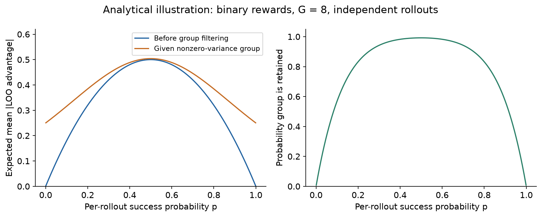
A practical reading is that $L_h$ estimates the contrast available in the accepted batch. It does not estimate contrast per second or per generated token. If two harnesses produce the same survivor signal but one requires many more discarded groups, equal scheduler scores can conceal very different costs. Logging the retention rate beside $L_h$ would expose this distinction without changing the policy objective.

4. Transferability: what gradient alignment actually predicts

4.1 The local argument behind the cosine

Let $\mathcal L_j$ be the loss associated with another harness, and let $g_h=\nabla\mathcal L_h$ be the selected harness’s gradient. Under an idealized SGD step of size $a$, a first-order expansion gives

$$\begin{aligned} \mathcal L_j(\theta-a g_h) &=\mathcal L_j(\theta) -a\nabla\mathcal L_j(\theta)^\top g_h+O(a^2)\\ &=\mathcal L_j(\theta) -a\|g_j\|\|g_h\|\cos(g_j,g_h)+O(a^2). \end{aligned} \tag{9}$$

A positive cosine predicts a local decrease of the other loss when the other assumptions hold. Normalizing by vector norms makes the comparison less dominated by an arm’s gradient magnitude. The resulting quantity answers a directional question rather than estimating the size of the improvement.

Several bridges remain between this argument and the paper’s deployment claim. The peer gradient is old, the vectors represent only some parameters, the optimizer is Adam rather than plain SGD, and evaluation uses a different task distribution. A decrease in a training surrogate also need not yield an immediate increase in task reward. The cosine is a cheap proxy whose usefulness must be demonstrated empirically, not a certificate of positive transfer.

4.2 Why the actual optimizer direction matters

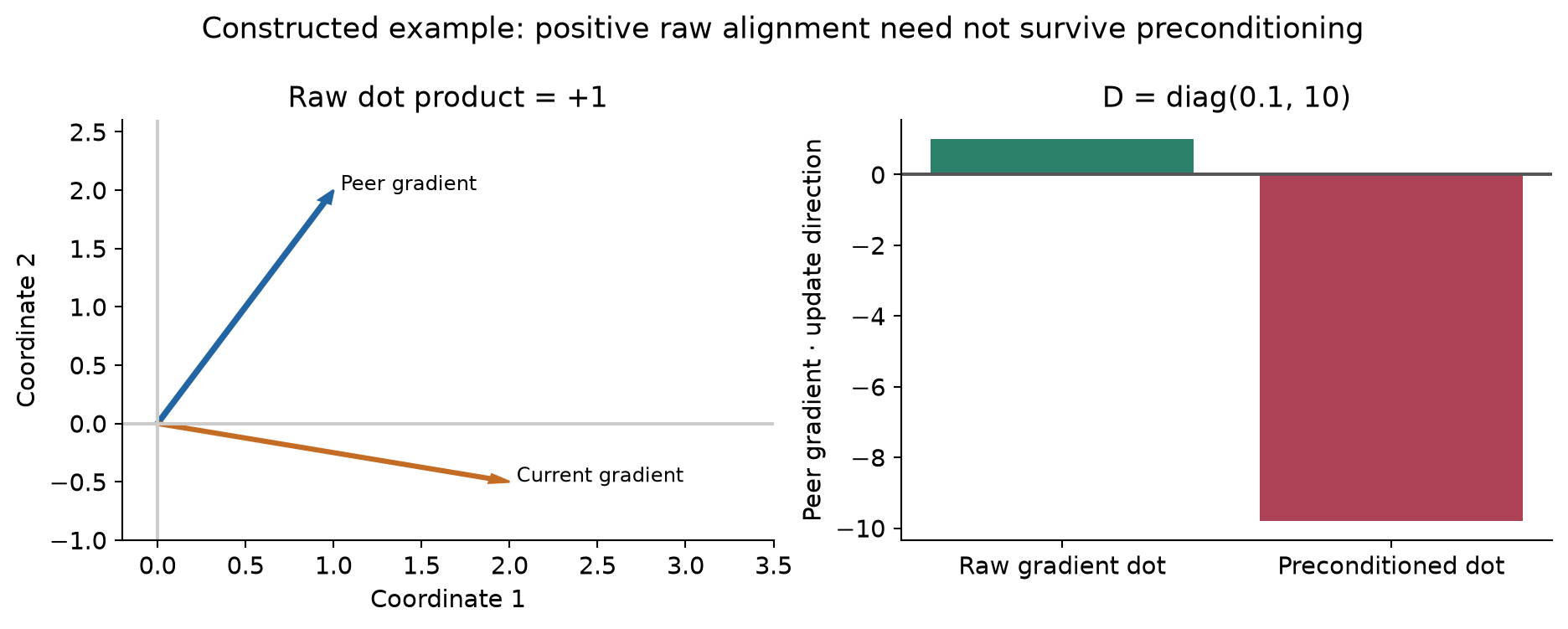
An Adam-like step can be written schematically as $\Delta\theta=-aD_tm_t$, where $m_t$ is a momentum estimate and $D_t$ is a diagonal adaptive scaling matrix. The first-order quantity relevant to a peer loss is then $g_j^\top D_tm_t$, not necessarily $g_j^\top g_h$.

For a constructed two-dimensional example, choose $g_j=(1,2)$ and $g_h=(2,-0.5)$. Their raw dot product is $2-1=1$, which is positive. If momentum is temporarily identified with the current gradient and $D=\operatorname{diag}(0.1,10)$, then

$$g_j^\top Dg_h=(1,2)^\top(0.2,-5)=0.2-10=-9.8. \tag{10}$$

The predicted sign reverses. This example does not show that Adam invalidates the reported results; it shows why a raw-gradient similarity should not be described as a guaranteed optimizer-level transfer metric. An informative comparison would measure raw-gradient and actual-update-direction alignment on the same batches.

The KL term introduces another interpretive issue. If the batch gradient includes a common regularization component, two harnesses may align partly because both are being pulled toward the reference policy. Such alignment is not necessarily irrelevant—it affects the real update—but it is weaker evidence of transferable task learning than alignment of the reward-dependent components alone. The paper does not provide a decomposition establishing how much of its signal comes from each source.

4.3 A fixed coordinate sketch, not a full gradient replica

Keeping six complete gradients is expensive. HarnessBandit restricts attention to the last four transformer blocks, excluding embeddings and the output head, then samples 65,536 coordinates. The coordinate allocation is proportional to each selected tensor’s number of elements, and the sampled positions remain fixed across steps. The paper motivates excluding the input and output matrices by their sensitivity to token frequency.

These choices reduce memory and communication while preserving a consistent coordinate system. Fixed positions are essential: taking different random positions each time and treating them as corresponding dimensions would destroy the meaning of a dot product. Proportional allocation avoids giving a tiny tensor the same number of sampled entries as a much larger tensor. It does not establish that all important gradient directions are equally well represented.

For intuition, suppose every coordinate in a $D$-dimensional selected subspace has inclusion probability $q=d/D$. With a common sampled set $I$,

$$\mathbb E\!\left[\sum_{k\in I}g_{h,k}g_{j,k}\right] =q\,g_h^\top g_j, \qquad \mathbb E\!\left[\sum_{k\in I}g_{h,k}^2\right] =q\|g_h\|^2. \tag{11}$$

The common scale is encouraging for dot products and squared norms. But cosine is a ratio of random quantities; a ratio of unbiased estimates is not automatically unbiased. Coordinate subsampling can miss concentrated signal. A dense random projection has different concentration properties, and invoking the general idea of sketching is not enough to transfer every projection guarantee to this particular sampling rule.

The additional restriction to the last four blocks is a second approximation. Alignment in that subspace may disagree with alignment in early layers or the omitted output head. That can be an acceptable engineering tradeoff, especially if late-layer directions are predictive, but it needs a sensitivity study over block selection and sketch size. The paper’s results establish performance of one configuration rather than independence from these choices.

4.4 Distributed reduction and peer memories

The selected sketch is reduced across data- and context-parallel ranks before being compared with other arms. Summing corresponding raw coordinates and then normalizing represents the global accumulated gradient. Normalizing each rank separately first would generally change the direction because small local gradients would receive disproportionate weight. A subsequent common world-size division does not change a cosine.

For each arm $j$, the scheduler stores a CPU exponential moving average $m_j$ of unit sketches. With update rate $\eta=0.3$, an observed arm receives

$$u_h=\frac{\hat g_h}{\|\hat g_h\|}, \qquad m_h\leftarrow(1-\eta)m_h+\eta u_h. \tag{12}$$

The current transfer signal is the mean cosine with initialized peers:

$$T_h=\frac{1}{|J_h|}\sum_{j\in J_h}\cos(\hat g_h,m_j), \qquad J_h=\{j\ne h:m_j\text{ exists}\}. \tag{13}$$

The comparison uses peer memories before updating the current arm’s memory. If no peer exists, transferability is unavailable and learnability supplies the score. Initialization, zero-norm sketches and zero-norm memories need explicit conventions in a complete numerical specification; one should not silently invent them when explaining the published equations.

The stored EMA need not have unit norm, even though its inputs do. Opposing recent directions can cancel and make its norm small. A cosine renormalizes that mean direction and can magnify the influence of noise when the mean nearly vanishes. A confidence measure based on memory norm or effective sample size would be a reasonable extension, but it is not part of the demonstrated result.

5. Turning two observations into a sampling distribution

5.1 Pooled normalization preserves comparison, but changes the scale over time

Learnability is nonnegative while cosine can be negative. The scheduler keeps separate pooled windows of the most recent 32 raw observations and min–max normalizes each coordinate. For a raw observation $x$ and its corresponding window $W_x$,

$$\tilde x=\operatorname{clip}\!\left( \frac{x-\min W_x}{\max W_x-\min W_x},0,1\right). \tag{14}$$

Pooling across arms retains between-arm differences. Per-arm normalization could make an objectively weak arm’s best recent observation look as good as a strong arm’s best observation. The paper sets a coordinate to 0.5 when fewer than two observations exist. Two or more identical observations also produce a zero denominator, however, and the equation does not specify that case. An epsilon, midpoint fallback or delayed update would each define a different numerical rule.

Normalization also removes absolute meaning. If all observed transfer cosines are negative, the least negative one can become one. It remains the best option in that recent window but is not thereby beneficial in the Taylor sense. If an extreme observation leaves the window, an unchanged raw value can acquire a different normalized score. The value EMA then mixes scores expressed relative to different historical ranges.

5.2 The fusion is a tradeoff, not a requirement that both signals be high

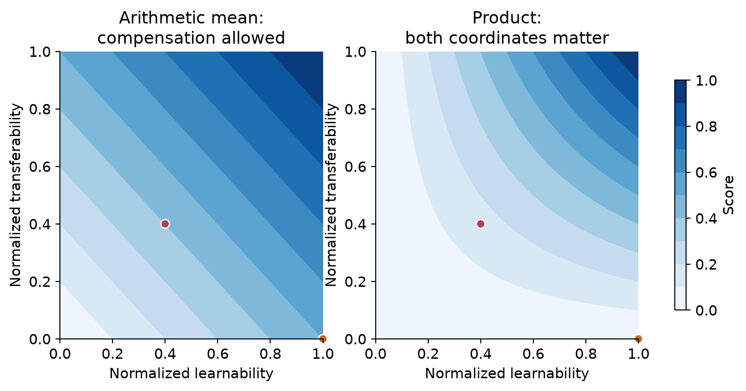
When both coordinates are available, the score is

$$S_h=\alpha\tilde L_h+(1-\alpha)\tilde T_h, \qquad \alpha=0.5, \qquad Q_h\leftarrow0.7Q_h+0.3S_h. \tag{15}$$

If only one coordinate is available, it supplies the score. An arithmetic mean permits compensation: $(\tilde L,\tilde T)=(1,0)$ scores 0.5 and outranks $(0.4,0.4)$, which scores 0.4. Thus the method balances the two properties; it does not enforce their conjunction. A product, minimum or transfer threshold would encode a stricter notion of jointly useful updates, at the cost of sensitivity to noise and normalization.

5.3 Exploration has three distinct components

The score used for sampling adds a count-dependent bonus:

$$U_h=Q_h+\frac{c}{\sqrt{n_h+1}},\qquad c=0.2. \tag{16}$$

The distribution combines temperature-scaled softmax with uniform exploration:

$$p_h=(1-\varepsilon) \frac{\exp(U_h/\tau)}{\sum_j\exp(U_j/\tau)} +\frac{\varepsilon}{H}, \qquad \tau=0.3,\quad\varepsilon=0.15. \tag{17}$$

The first 30 steps are round-robin warmup, giving five scheduled visits to each of six arms. At selection time, an unvisited arm is assigned the current maximum value rather than an artificially low score. After warmup, the inverse-square-root bonus favors low counts, while the explicit floor prevents any arm’s probability from becoming zero.

These mechanisms should not be conflated with a standard UCB regret guarantee. The bonus lacks a growing global-time term. An arm’s count bonus stays fixed while it is not selected, and the shared policy changes every arm’s utility whenever any arm trains. This is a nonstationary allocation heuristic, not a solution to the classical fixed-reward bandit problem.

For six arms, the uniform floor is $0.15/6=0.025$. If an arm stayed exactly at that floor, its expected waiting time would be 40 steps. Its probability of receiving no visit in 32 steps would be $0.975^{32}\approx0.445$. With a probability at least as large as the floor, this expression is an upper bound, not a prediction of the actual run. Exploration guarantees a positive chance, not fresh measurements on every short interval.

5.4 Two clocks govern memory

An EMA with rate 0.3 halves the weight of an old observation after

$$k_{1/2}=\frac{\log(0.5)}{\log(0.7)}\approx1.94 \tag{18}$$

subsequent updates to that EMA. Those are visits to the same arm, not global training steps. Under uniform six-arm sampling, this corresponds loosely to about 11.7 global steps; a neglected arm can retain an old direction much longer. Meanwhile, the normalization window contains 32 pooled observations, not 32 observations per arm.

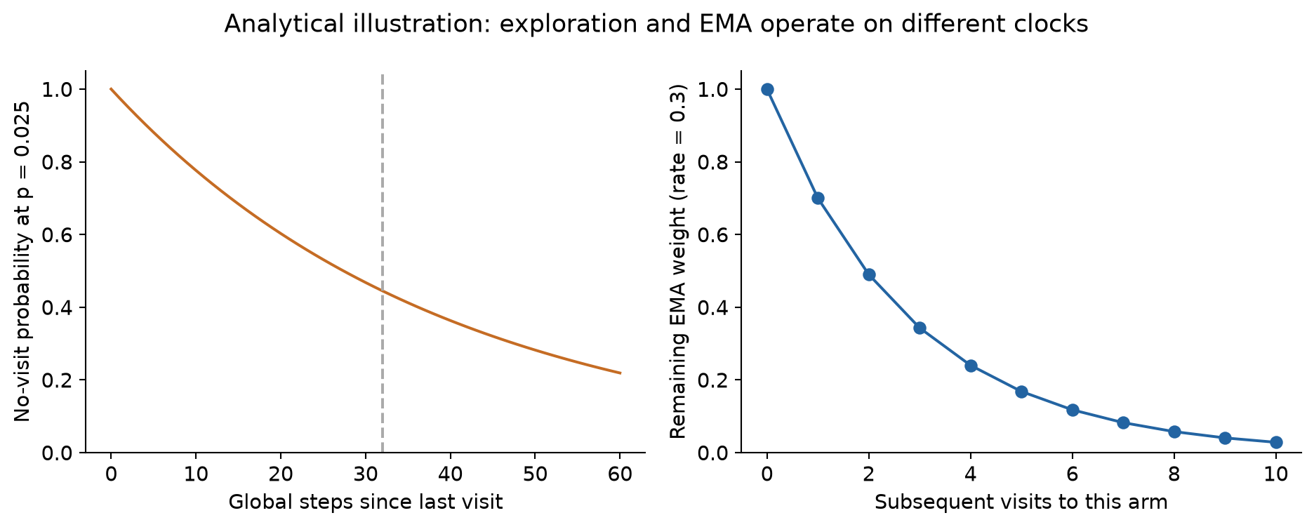
This mismatch creates a feedback loop. An old peer direction affects today’s transfer score; that score affects who is sampled; infrequently sampled peers remain old. The warmup initializes the memories but does not solve later staleness. Recording each memory’s age and testing age-aware comparison would directly investigate this failure mode.

6. Algorithm and resource accounting

6.1 Numbered pseudocode for one scheduling cycle

The following is a conceptual reconstruction of the method, not executable training software. It separates the gradient observation from the later use of the observation. The paper’s unspecified degenerate normalization cases remain explicit rather than being hidden in a purportedly exact implementation.

Algorithm 1 — HarnessBandit around an existing on-policy trainer

01  Create one shuffled task pool and leftover-group buffer per harness.
02  Fix the sampled gradient coordinates; initialize counts and memories.
03  Initialize pooled L/T windows and per-arm score values.
04  For optimizer step t = 1, ..., T:
05      If t <= 30, select the next arm in round-robin order.
06      Otherwise form U, apply softmax and the uniform floor; sample h.
07      Collect a pure h batch; filter zero-variance reward groups.
08      Reuse eligible leftover groups from the buffer for h.
09      Compute group-relative advantages and the hierarchical mean L.
10      Accumulate backward passes for the unchanged policy loss.
11      Capture the fixed-coordinate sketch; reduce across parallel ranks.
12      Compute T against initialized other-arm gradient memories.
13      Perform the trainer's optimizer update on the shared policy.
14      Update pooled windows; normalize available observations.
15      Fuse observations; update Q[h], count[h] and gradient memory[h].
16      Save scheduler diagnostics alongside the training-step record.

Line 7 is more than a data-loader detail. If a harness cannot produce enough nonconstant groups, waiting for a full batch may dominate the cost of a scheduled visit. The leftover buffers reduce unnecessary waste from oversampling and preserve the arm identity of retained groups. Their existence should not be mistaken for proof that all arms consume identical raw sampling budgets. A complete comparison should report generated, scored, retained and actually optimized trajectories separately.

The scheduler is naturally compatible with tools that expose a consistent trajectory format to the learner while leaving the external harness black-box. Polar provides this systems context in the paper’s setup. The key separation is between the serving boundary, where the agent conducts an interaction, and the learner, where generated actions receive token masks, rewards and policy ratios. Harness selection sits above both boundaries and decides which interaction source to request next.

6.2 What the published configuration costs

The experiment uses Qwen3.5-2B, four GPUs with context parallelism of four, 150 optimizer steps, eight prompt groups per batch and eight trajectories per group. The reported learning rate is a constant $10^{-6}$, with KL coefficient 0.05, maximum response length 8,192 and maximum prompt length 40,000. These limits make tool-heavy trajectories possible, but they also make per-step latency sensitive to actual lengths and tool behavior.

A simple multiplication gives a nominal accepted-trajectory budget:

$$150\times8\times8=9{,}600. \tag{19}$$

This is an accounting calculation under full batches, not a claim that exactly 9,600 trajectories were generated. Filtering and oversampling can increase the raw total; buffers change when already generated trajectories are used. Nor does equal trajectory count imply equal token count or equal wall time. The experiments are described as sharing a 150-step budget, and that is the safest common-budget statement to retain.

The persistent gradient-memory footprint is comparatively modest. Six float32 vectors of length 65,536 require

$$6\times65{,}536\times4=1{,}572{,}864\ \text{bytes}=1.5\ \text{MiB}. \tag{20}$$

This excludes current sketches, reduction buffers, coordinate indices and the trainer’s normal optimizer state. Pairwise comparisons cost on the order of $Hd$ per selected step, and one sketch must be gathered and reduced. Reusing an existing backward pass is cheaper than computing fresh counterfactual gradients for all arms. Still, the paper does not report a measured end-to-end overhead or training speedup that would justify a numerical efficiency claim.

7. Results: separate adaptation, transfer and repeatability

7.1 Two evaluation protocols answer different questions

PinchBench evaluates 147 held-out tasks, one run each, through OpenClaw. OpenClaw appeared in training, so this tests new tasks under a familiar interface. ClawEval evaluates 161 held-out tasks through its own native loop, with three trials per task. The latter additionally changes the interface. Neither benchmark directly measures uniform performance over all six training harnesses.

For three attempts, “all three succeed” and “at least one succeeds” are very different properties. The paper denotes them Pass³ and pass@3 respectively. The former is closer to repeatability on the evaluated attempts; the latter rewards the ability to reach a successful trajectory within a small sampling budget. These should not be merged into a single generic success-rate statement.

Method	Pinch mean	Claw all 3	Claw any 3	Claw score
Untuned base	0.330	43/161	58/161	0.534
Mixed 2	0.493	32/161	48/161	0.490
Mixed 6	0.331	35/161	62/161	0.510
HarnessBandit	0.506	43/161	67/161	0.556

These are Table 1’s values. Relative to the two-harness mixture, the Pinch gain is 0.013, or 1.3 percentage points on the score scale. Relative to the six-harness mixture, it is 0.175, or 17.5 points. Relative to the base model, it is 17.6 points. The distinction matters because prose in the paper blurs some baseline associations and uses 17.6 where the table arithmetic for the six-harness comparison gives 17.5.

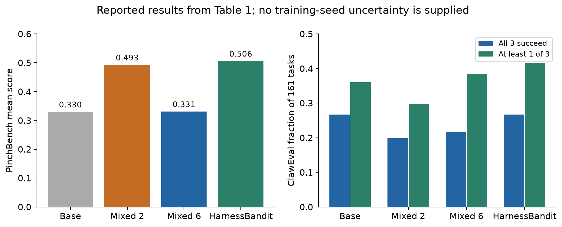
ClawEval’s at-least-one count rises by five tasks over the six-harness mixture, a difference of $5/161\approx3.11$ percentage points. It rises by nine tasks over the base model. Yet the all-three count only returns to the base model’s 43. The result supports improved sampled coverage with recovered repeatability relative to the mixtures. It does not show that all aspects of reliability improve over the base policy.

The two mixtures illustrate why adaptation alone is an incomplete objective. The two-harness mixture gains substantially on the familiar-interface benchmark but drops on ClawEval. The six-harness mixture preserves more ClawEval sampling coverage but nearly loses the Pinch gain. HarnessBandit obtains a better joint outcome in this reported run. The table does not determine whether the advantage comes chiefly from the two signals, pure batches, a fortunate allocation, or interactions among these changes.

7.2 Category results reveal a real tradeoff

Appendix B breaks PinchBench into categories. Compared with the two-harness mixture, HarnessBandit improves skills from 0.367 to 0.676 and integrations from 0.191 to 0.364. Memory falls from 0.913 to 0.637, while CSV analysis falls from 0.433 to 0.352. Coding changes slightly, from 0.673 to 0.661. These are not uniformly positive changes masked by an awkward overall metric.

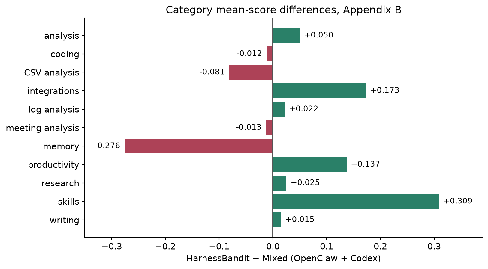
This suggests a deployment question more useful than simply asking whether 0.506 is better than 0.493: is the resulting category tradeoff suitable for the intended agent workload? A memory-heavy assistant could value the lost category performance more than the average gain. Conversely, a tool-integration workload may prefer the new balance. The scheduler currently optimizes proxy signals, without explicit deployment-category weights or worst-category constraints.

The six-harness mixture has a reported zero in the writing category. That is a result for this evaluation configuration and run, not evidence that the trained model has lost all ability to write. Sparse categories and single-attempt evaluation can produce unstable averages. The paper supplies some category sizes, such as 14 coding and 26 CSV tasks, but not enough information to reconstruct every category’s statistical uncertainty from the table alone.

7.3 What the scheduler diagnostics show—and do not show

The normalized signal summaries place Pi high on learnability, around 0.75, but at about 0.49 on transferability. OpenCode is around 0.62 and 0.60, and OpenClaw around 0.55 and 0.59. Qwen Code is lower, around 0.53 and 0.37. These summaries are consistent with the intended balancing mechanism. They are not causal evidence that a higher transfer score predicts a larger held-out reward improvement.

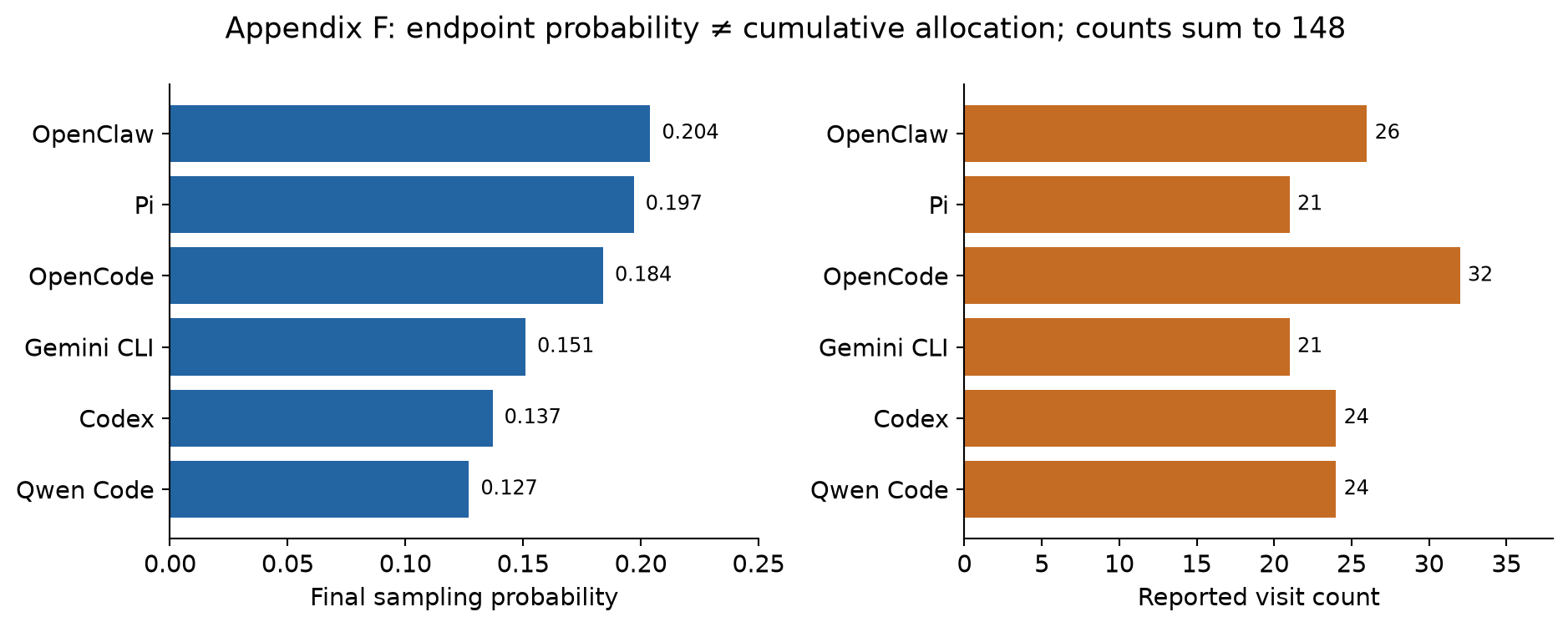
The reported average sampling probabilities favor OpenCode and OpenClaw at roughly 0.21 and 0.18. Final probabilities tell a different story: OpenClaw is 0.204, Pi 0.197 and OpenCode 0.184. An endpoint probability is a preference for the next draw, whereas a count integrates the realized history. Pi can end with high probability despite receiving relatively few earlier visits.

The pairwise gradient plots also require care. They compare a current source sketch against target memories measured at different times. This is a directed, asynchronous observation matrix. It need not be symmetric even though the cosine of two fixed vectors is symmetric. Near-zero cosines with changing signs should be interpreted as weak, noisy directional evidence, especially after min–max normalization stretches them across the full score range.

8. Limitations and numerical questions that remain open

The reported training study uses one small model scale and a short horizon. It does not establish robustness across larger policies, different task universes, alternative reward definitions or many independent training seeds. The two evaluation suites provide useful distribution shifts, but they do not exhaust the six interfaces or prove robustness to arbitrary new harnesses.

The baseline design also leaves identification incomplete. A uniform pure-batch scheduler would isolate the benefit of pure batches from the benefit of adaptive allocation. A round-robin pure-batch schedule would remove sampling variance while keeping arm attribution. Learnability-only and transfer-only variants would show whether both signals are necessary in this harness setting. Results from related domain-curriculum papers cannot substitute for those ablations here.

Two appendix issues particularly affect reproducibility of the explanation:

1. Signal scale. Appendix D’s raw learnability plot is roughly in the 0.60–0.95 range. Under the simplest stated combination of rewards in $[0,1]$, unscaled leave-one-out advantages and $G=8$, Equations 1–5 bound the group mean absolute advantage by about 0.5714. Filtering cannot exceed a per-group bound. Some additional reward transformation, advantage definition, aggregation or plotting convention is needed to reconcile the statements. This is a request for the exact logged quantity, not proof that the training result is invalid.
2. Training counts. Appendix F lists counts 32, 26, 24, 24, 21 and 21, totaling 148, and describes 148 observations after warmup. A 150-step run with 30 warmup steps instead has 120 post-warmup steps. Different event types could explain some discrepancy, but the paper does not clearly connect selected steps, successful updates and logged observations. It would be inappropriate to fabricate the missing accounting.

There are also smaller specification gaps: a zero-range normalization window, zero-norm sketches, the age of retained rollout groups, and the precise relationship between scalar scheduling weights and loss weighting. These do not all imply practical failures. They define the boundary between a clear conceptual method and an unambiguous numerical recipe.

9. Critical analysis: the real contribution is a measurable allocation hypothesis

9.1 A promising separation of local opportunity and shared direction

The strongest idea is to distinguish reward contrast from cross-interface compatibility while reusing information already produced by training. This makes the method easier to justify than a scheduler that uses only absolute task reward. High success can mean saturation; large contrast can mean a useful local gradient; positive alignment can suggest compatibility. The separation creates testable hypotheses about how an interface contributes to a shared policy.

The weakest leap is to treat the fused score as a faithful surrogate for long-run generalization. Learnability is conditioned on the accepted batch, transferability is estimated from stale partial gradients, normalization removes absolute scale, and the optimizer transforms directions. Each approximation may be reasonable individually. Their composition needs calibration against actual subsequent outcomes, not just a plot showing that probabilities change.

A direct calibration study would record a signal at step $t$, then evaluate changes on a small fixed probe collection after controlled updates. The study should test whether the cosine predicts peer loss reduction and whether that reduction predicts task reward. A proxy can be useful even when neither relationship is perfect, but the evaluation would reveal which link limits it.

9.2 The decisive ablations should preserve the surrounding system

My proposed first experiment keeps the same pools, group filter, pure batches, optimizer and accepted-trajectory budget, then compares uniform random selection, round-robin selection, learnability-only allocation, transfer-only allocation and the fused scheduler. This avoids attributing a systems change to a bandit signal. Repeating each configuration with several training seeds is necessary to distinguish allocation benefits from favorable rollout randomness.

A second experiment holds the allocation rule fixed while varying the transfer observation: current versus age-limited peer memories, raw gradients versus optimizer-step directions, late blocks versus several block ranges, and coordinate subsampling versus a suitable random projection. These changes answer different questions and should not all be bundled into a single improved variant. Memory norms and observation ages should be reported alongside the cosines.

A third experiment matches wall time or generated tokens instead of only optimizer steps. It should report the full funnel from requested groups to successful tool sessions, scored groups, retained groups and optimized trajectories. If the survivor signal selects expensive low-yield interfaces, the best step-budget scheduler may not be the best cost-budget scheduler. A candidate cost-aware objective would divide an estimated utility by expected resource use, but that is an extension to be tested, not a result established here.

9.3 Coverage gains and reliability gains deserve separate acceptance criteria

For the five-task ClawEval gain over the six-harness mixture, aggregate counts alone are insufficient for a paired significance test. We need to know which tasks change from failure to success and which regress. Likewise, identical all-three totals do not imply that the same 43 tasks remain reliable. Marginal counts conceal potentially important exchanges between capabilities.

A more informative deployment report would preserve task-level paired outcomes, evaluate more than three attempts where feasible, and show category-level regressions alongside mean gains. For high-cost tool actions, consistency may deserve more weight than sampled coverage. The training allocation criterion could eventually reflect that priority, but the present proxy does not directly encode it.

Finally, “bandit” should be understood as the organizing abstraction for online selection. This is not a new regret theorem, not lossless training, and not inference-time acceleration. Selecting a different harness changes the training distribution and therefore the model learned. The attractive claim is narrower: inexpensive observations of local contrast and cross-interface direction can help allocate a limited RL training budget.

10. Conclusion

HarnessBandit moves adaptation pressure into the choice of execution interface. A pure batch makes each gradient attributable to one harness; absolute advantages estimate local opportunity; compact gradient memories estimate directional compatibility; a smoothed score and exploration floor distribute future updates. The reported run achieves a useful balance between familiar-interface adaptation and held-out-interface performance.

The method is most convincing as an allocation hypothesis with a low additional information cost. Its practical interpretation depends on understanding filtered advantages, stale sketch geometry and the difference between one-of-three success and three-of-three success. The next evidence needed is a controlled pure-batch ablation, a complete resource ledger, repeated training runs and clarification of the appendix’s signal and count definitions.

References and further reading

• Wei et al. HarnessBandit, arXiv:2609.13739v1. Primary source; main text, Table 1 and Appendices A–F.
• Xu et al. Polar: Agentic RL on Any Harness at Scale. Systems context for harness-independent agentic RL. Official resource linked by the paper.
• Yang et al. Transferability for General Reasoning: An Automated Curriculum for Multi-Domain RLVR. Related two-signal curriculum over reasoning domains; its experiments are not HarnessBandit ablations.

All eight figures in this review were drawn for the review. Figures based on reported measurements identify their source table or appendix; analytical figures illustrate explicitly stated assumptions. No new model training or empirical replication result is claimed.