STAR-KV: Learning the Rank Is Only Half of KV Cache Compression

Review date: 2026-11-01 · Author: Zhongzhu Zhou
Paper reviewed: STAR-KV: Low-Rank KV Cache Compression via Soft Thresholding for Adaptive Rank Control
Paper authors: Priyansh Bhatnagar, Ashkan Moradifirouzabadi, Se-Hyun Yang, SeungJae Lee, Jungwook Choi, Mingu Kang
arXiv: 2606.08382 · Version: v1, 2026-06-07

1. Three decisions hidden inside one compression ratio

A KV cache with one quarter of its original channels is not automatically a fast cache. The missing channels may carry information that a particular attention head needs; reconstructing them can consume more time than the reduced memory traffic saves; quantizing the retained coordinates can damage precisely the directions that survived the rank selection. STAR-KV addresses these three decisions together: how much rank to retain, how to arrange the factors, and how to store and consume the resulting latent cache.

The paper learns spectral thresholds at fine granularity, uses head-wise decomposition for keys and joint decomposition for values, and combines the resulting representation with structured rotation and mixed-precision quantization. Custom attention kernels then avoid materializing large reconstructed intermediates. The contribution is therefore a coupled model-and-system design. An account that reduces it to “take the top singular vectors” misses both the optimization and the runtime transformation.

Two qualifications belong at the beginning. First, this is a lossy, trained compression method. Appendix A.3 assigns learning rates to model parameters as well as to thresholds, and follows the compression-aware phase with additional distillation. It is not just a fixed pretrained model with a cache-format switch. Second, the largest reported attention speedup, 6.9× on an RTX 4090, uses an extrapolated dense baseline because that baseline does not fit at the target context length. The paper also contains measured-baseline results, which are valuable but answer a narrower performance question.

This review uses the full 20-page v1, including the proofs, calibration settings, extra evaluations, and kernel discussion. Paper measurements are distinguished from the analytical examples below. The aim is to explain which parts are algebraically exact, which parts are learned approximations, and where the empirical evidence leaves uncertainty.

2. Prerequisites: what is actually being compressed?

2.1 Cache size and the difference between rank and bits

For batch size $B$, sequence length $T$, $L$ layers, $h_{kv}$ KV heads, head dimension $d_h$, and $b$ bits per stored scalar, a uniform dense cache has the following payload size in bytes:

$$M_{\mathrm{KV}}=2BTLh_{kv}d_h\frac{b}{8}. \tag{1}$$

The factor two counts keys and values. This expression excludes weights, temporary buffers, allocator rounding, and quantization metadata. In grouped-query attention, the number of KV heads—not the larger query-head count—belongs in this storage formula. Using the query count would overstate the dense memory available to save.

A rank reduction changes the number of stored coordinates. Quantization changes the bits per coordinate. Token eviction changes the number of stored time steps. These operations act on different axes, so their ideal payload reductions can multiply, while their quality losses and runtime costs interact. STAR-KV primarily reduces channels; it does not rely on dropping tokens in its main configuration.

Throughout this review, $\rho$ denotes the retained rank fraction and $c=1-\rho$ the removed fraction. Thus “75% compression” means $\rho=0.25$, corresponding to a 4× ideal reduction at unchanged precision. This convention prevents confusion with papers that call a retained fraction a compression ratio.

2.2 From a projection weight to a latent cache

Use row-vector activations and let a projection weight be $W\in\mathbb R^{d_o\times d_i}$. Its truncated SVD gives

$$W_r=U_r\Sigma_rV_r^\top, \qquad Z=XV_r\Sigma_r, \qquad \widehat K=ZU_r^\top. \tag{2}$$

For $X\in\mathbb R^{T\times d_i}$, the latent cache $Z$ has shape $T\times r$, while the reconstructed keys have shape $T\times d_o$. The smaller object is retained across decoding steps. The factors are model-side objects that do not grow with sequence length. A useful runtime design consumes $Z$ without writing the full reconstructed cache back to global memory.

Weight-space SVD and activation-space approximation are different objectives. With residual $E_W=W-W_r$ and empirical second moment $C_X=X^\top X$, the activation error is

$$\|XE_W^\top\|_F^2 =\operatorname{tr}(E_W C_X E_W^\top). \tag{3}$$

Ordinary weight SVD minimizes an unweighted matrix error; actual activations weight directions through $C_X$. STAR-KV’s distillation supplies a data-dependent learning signal on top of the spectral parameterization. That signal helps, but it does not turn a spectral theorem into a theorem about answer accuracy.

2.3 Why key error and value error behave differently

For a single head, write $a=qK^\top/\sqrt{d_h}$, $p=\operatorname{softmax}(a)$, and $o=pV$. Perturbing keys changes the probabilities; perturbing values changes what those probabilities aggregate. A first-order expansion is

$$\delta o\approx \left(\delta a\,[\operatorname{diag}(p)-p^\top p]\right)V +p\,\delta V, \qquad \delta a=\frac{q\,\delta K^\top}{\sqrt{d_h}}. \tag{4}$$

Here $p$ is a row vector. The omitted term includes products of perturbations. This equation explains why equal reconstruction error does not imply equal functional error: query alignment, probability concentration, and value magnitude all matter. It also explains why a successful average on common-sense tasks cannot guarantee preservation of a rare retrieval dependency.

3. Learning a rank through a spectral threshold

3.1 Hard selection and its trainable surrogate

For descending singular values $\sigma_j$, a threshold $\alpha$ defines a discrete retained rank:

$$r(\alpha)=\sum_j\mathbf 1\{\sigma_j\geq\alpha\}, \qquad \widetilde\sigma_j=\sigma_j\mathbf 1\{\sigma_j\geq\alpha\}. \tag{5}$$

The indicator changes only when the threshold crosses a singular value. Its ordinary derivative cannot provide a useful smooth optimization signal. STAR-KV replaces the hard selection during training with the following piecewise transform, using the paper’s choice of a zero lower branch:

$$T_s(\sigma;\alpha)= \begin{cases} \sigma\tanh\!\left(s(\sigma-\alpha)\right),&\sigma\geq\alpha,\\ 0,&\sigma<\alpha, \end{cases} \qquad s>0. \tag{6}$$

Large singular values sufficiently above the threshold are nearly preserved. Values close to the threshold are attenuated before they disappear. This is a transition in singular-value space, not a token importance score and not a per-request top-$k$ selection. The learned deployment ranks remain properties of the prepared model.

For a fixed singular value strictly above the threshold,

$$\frac{\partial T_s}{\partial\alpha} =-s\sigma\,\operatorname{sech}^2\!\left(s(\sigma-\alpha)\right). \tag{7}$$

The gradient is concentrated near the threshold. Increasing $s$ sharpens the decision but also localizes the useful learning signal. Far below the threshold, the lower branch gives zero gradient with respect to $\alpha$ through that component. Far above it, the hyperbolic tangent saturates. Threshold initialization and spectral scale therefore affect optimization even though rank itself is dimensionless.

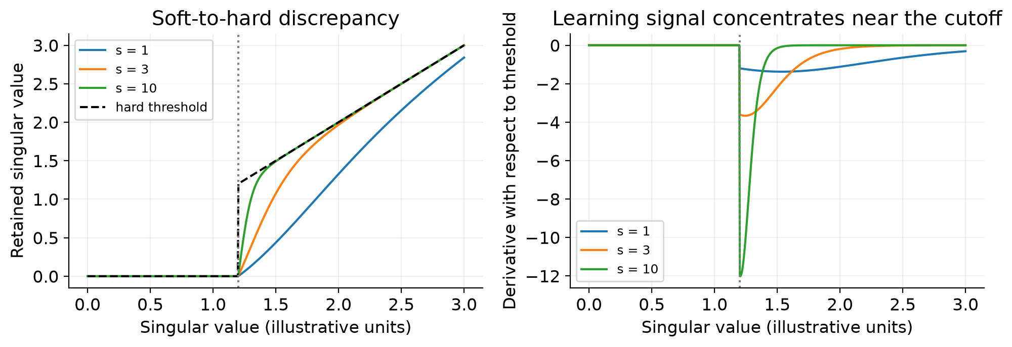
Figure 1. Original analytical illustration of equations (6)–(7), with an arbitrary threshold of 1.2 and three slopes. These curves are not model measurements. The hard rule preserves the original singular value above the cutoff; the training surrogate attenuates it.

The function is continuous at the boundary when the lower branch is zero, but is generally not differentiable there: the two one-sided derivatives differ. It is better described as differentiable almost everywhere than globally smooth. This does not make gradient-based learning unusable; it does matter when interpreting the mathematical claim.

A second distinction concerns conversion to deployment. A surviving singular value is shrunk during the soft phase but restored by the hard rule in equation (5). Near the threshold, this discrepancy can be large. Equality is an especially sharp boundary: the soft value is zero, while the displayed hard convention includes the component. In practice one needs an explicit convention and quality measurement after conversion. The paper’s stabilization phase is relevant, but it does not by itself provide a bound on this conversion error.

3.2 Distillation versus pressure to compress

The training objective combines teacher-to-student KL divergence with a threshold penalty:

$$\mathcal L= D_{\mathrm{KL}}(p_{\mathrm{teacher}}\|p_{\mathrm{student}}) +\gamma\mathcal L_{\mathrm{cmp}}, \qquad \mathcal L_{\mathrm{cmp}}= \sum_{\ell,h}e^{-\alpha^K_{\ell,h}}+ \sum_\ell e^{-\alpha^V_\ell}. \tag{8}$$

The KL term resists output changes on calibration examples. Minimizing the exponential term pushes thresholds upward and therefore tends to discard more singular directions. The student can also adapt its weights to reduce the damage. This competition is the mechanism behind adaptive allocation; the penalty is not a direct measurement of runtime or cache bytes.

For one threshold, the penalty gradient is $-\gamma e^{-\alpha}$. Its magnitude decays as the threshold grows. Equal threshold increments need not remove equal numbers of singular values, and equal removed ranks need not save equal latency in different kernels. Consequently, equation (8) is a compression surrogate, not an explicit constrained optimization that guarantees an arbitrary requested byte budget.

The hybrid factorization creates one key threshold per head per layer and one joint value threshold per layer. Counting terms therefore gives the key side more threshold variables. The final balance depends on spectra, task gradients, and the regularization scales. A fair interpretation is that the chosen objective finds useful allocations in the reported experiments, rather than that the scalar $\gamma$ universally identifies an optimal rank budget.

4. Calibration is model adaptation, not just threshold fitting

Appendix A.3 changes the practical interpretation of the method. AdamW uses a learning rate of $2\times10^{-5}$ for model parameters and $10^{-2}$ for the adaptive thresholds. The calibration set contains 3,000 FineWeb-Edu samples. The first phase runs for one epoch with the combined objective; the compression penalty is then disabled for another 1,000 optimization steps with distillation only. It would be inaccurate to describe this procedure as updating only a few threshold scalars.

Sequence length is 8,192 for LongChat and the tested LLaMA-3/3.1 models, and 4,096 for LLaMA-2-7B. Layers 0, 1, and 31 are exempted from compression. This exception is important: a sensitive early or final layer cannot lose rank if it is protected in advance. The learned profile combines adaptive choices with a manually fixed boundary condition.

The main text describes a cost below six GPU-hours, whereas Appendix A.3 reports approximately six GPU-hours for one epoch on a setup with two RTX PRO 6000 GPUs. The appendix also specifies the subsequent 1,000 steps. These statements do not unambiguously establish an all-inclusive end-to-end preparation cost. The defensible description is a modest calibration procedure in the authors’ setup, with incomplete accounting of every phase; six GPU-hours should not silently become a universal total-cost guarantee.

Algorithm 1. Prepare a compressed model

The numbered procedure below summarizes the paper’s phases. It does not add a claim about an unreported optimizer schedule or exact stopping rule.

1. Load the pretrained model and retain its teacher outputs.
2. Keep layers 0, 1, and 31 outside the compression set.
3. Factor each compressible key head and each joint value map.
4. Introduce spectral thresholds and the soft transform.
5. For one epoch over 3,000 calibration samples:
   a. Evaluate teacher and compressed-student distributions.
   b. Form KL distillation plus the threshold penalty.
   c. Update model parameters and thresholds with AdamW.
6. Disable the compression penalty.
7. Continue distillation for 1,000 optimization steps.
8. Convert the learned spectral selection into compact factors.
9. Prepare value/output fusion and optional rotated quantization.
10. Evaluate the final deployed representation and its memory use.

Step 10 is essential reasoning for any use of the method: the final compact representation is the object that must meet quality and storage requirements. A small training loss alone is not a deployment result. The paper does not expose every detail of the transition between the stabilization and final hard selection in its prose, so this summary deliberately avoids inventing a more specific ordering.

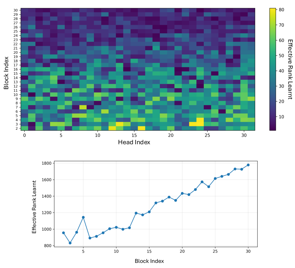
Figure 2. Cropped and vertically arranged from Bhatnagar et al., Figures 10–11, arXiv:2606.08382v1, CC BY 4.0. The upper panel allocates key rank per head and layer; the lower panel allocates joint value rank per layer, at the reported 75% compression setting. Their rank scales differ.

The maps show why a uniform retained fraction can waste the budget. Some key heads receive substantially more coordinates than others, while value ranks vary across depth. However, a color map is not a direct sensitivity measurement: it is the outcome of a particular training objective, protected-layer policy, calibration distribution, and optimization path. Its shape alone cannot establish that those ranks transfer safely to a different model.

The appendix supplies more useful evidence about stability. On LongChat, changing FineWeb-Edu to C4 changes key ranks by an average of 1.6 out of 128 per head and value ranks by 20 out of 4,096 per layer. RedPajama gives corresponding deviations of 1.7 and 7.7. Across LLaMA-2-7B and LLaMA-3.1-8B, normalized key and value profile deviations are reported as 3.2% and 11.4%. The larger value deviation is a reason to be cautious about transferring one profile wholesale. Similar profile statistics also do not establish identical task errors.

5. Why keys and values use different decompositions

5.1 The reconstruction bill

Let $h$ heads each have width $d_h$, giving combined width $d=hd_h$. At a retained fraction $\rho$, joint decomposition uses rank $R=\rho d$, whereas head-wise decomposition uses rank $r=\rho d_h$ per head. Both store the same total number of latent coordinates in this simplified equal-rank comparison.

Explicitly reconstructing $T$ cached positions has multiplication counts proportional to

$$C_{\mathrm{joint}}\propto TRd =T\rho h^2d_h^2, \qquad C_{\mathrm{head}}\propto hTrd_h =T\rho hd_h^2. \tag{9}$$

Their ratio is $h$. This is a ratio of reconstruction work, not a claim that the whole attention layer becomes $h$ times faster. It omits projection costs, memory traffic, parallelism, kernel launch overhead, and opportunities to eliminate reconstruction through algebraic rearrangement. Nevertheless, it identifies why joint decomposition can be expensive if its larger latent space must be expanded separately at every cached token.

5.2 What joint decomposition guarantees—and what it does not

For a column-partitioned matrix $W=[W^{(1)},\ldots,W^{(h)}]$, concatenate head-wise approximations of rank at most $r$. The resulting matrix satisfies

$$\operatorname{rank}\!\left([\widehat W^{(1)},\ldots, \widehat W^{(h)}]\right) \leq\sum_{i=1}^{h}\operatorname{rank}(\widehat W^{(i)}) \leq hr=R. \tag{10}$$

Every head-wise candidate is therefore feasible for the unrestricted joint rank-$R$ approximation. Taking the minimum over the larger feasible set yields

$$\min_{\operatorname{rank}(Y)\leq R}\|W-Y\|_F \leq \min_{\operatorname{rank}(Y_i)\leq r} \|W-[Y_1,\ldots,Y_h]\|_F. \tag{11}$$

This is the clean feasible-set argument in Appendix A.2. It establishes a matrix reconstruction advantage at equal total rank. It says neither that joint decomposition has lower runtime nor that it yields smaller attention-output error on every input. It also compares with equal head-wise rank constraints; learned nonuniform allocations require their own budget accounting.

The paper additionally examines normalized singular spectra. For the best rank-$r$ approximation in spectral norm, relative error is $\sigma_{r+1}/\sigma_1$. The plotted LLaMA-2-7B key matrices have faster-decaying normalized spectra than the value matrices. That observation motivates spending the more expressive joint approximation on values and accepting the cheaper head-wise approximation on keys.

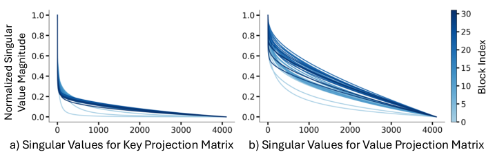
Figure 3. Paper Figure 6, cropped; Bhatnagar et al., CC BY 4.0. Curves cover the 32 LLaMA-2-7B blocks and normalize each matrix by its largest singular value. These are weight spectra, not measured task sensitivity curves.

The rationale combines empirical spectra with an exact approximation inequality. Keeping those two evidence types separate matters. A spectrum can be concentrated even if a small singular direction is important to a particular query distribution. Equation (3) and the attention perturbation in equation (4) explain why output calibration remains necessary.

5.3 Values permit a useful reassociation

Let joint latent values be $Z_V\in\mathbb R^{T\times R_V}$. A head’s reconstructed values are $Z_VU_h^\top$, and let $O_h\in\mathbb R^{d_h\times d}$ be its block of the output projection. Then

$$p_h(Z_VU_h^\top)O_h =(p_hZ_V)(U_h^\top O_h). \tag{12}$$

The right-hand factor can be prepared offline. The left side reconstructs a $T\times d_h$ value matrix before aggregation; the right side first aggregates into one latent row. This removes a reconstruction cost that grows with context length. It does not make output projection free, and it does not remove the approximation already introduced by rank truncation.

With shared joint latent values, stack the distinct per-head probabilities into $P\in\mathbb R^{h\times T}$. Computing $PZ_V$ turns multiple vector-style reductions into a matrix multiplication, improving reuse and arithmetic intensity. Each row still contains its own attention distribution. Sharing values does not mean sharing attention probabilities across heads.

Keys are harder. Rotary position encoding inserts a different rotation for each cached position. In column-vector notation, a score contains $q_t^\top R_t^\top R_jU_Kz_j$. The factor between the query and latent key depends on $j$, so a single position-independent offline fusion cannot simply absorb it for every token. STAR-KV retains pre-RoPE latent keys and fuses reconstruction, rotation, and scoring at runtime.

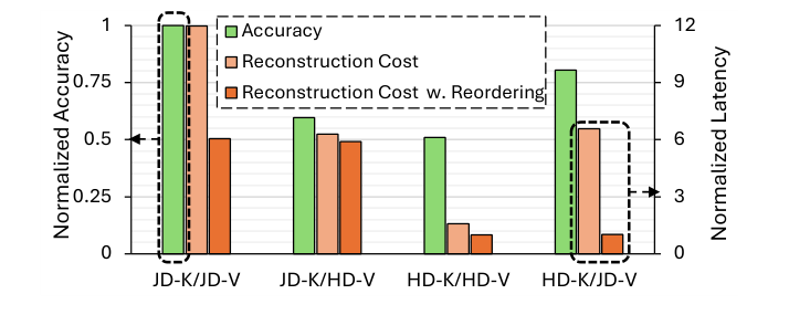
Figure 4. Paper Figure 7, cropped; Bhatnagar et al., CC BY 4.0. Accuracy uses the left axis; reconstruction latency uses the right axis. Output reordering makes HD-K/JD-V attractive in the measured setting. The normalized bars are not end-to-end generation throughput.

This is why the hybrid choice is more than a compromise between two reconstruction errors. It exploits an asymmetry in what can be moved out of the sequence-length-dependent path. Alternatives remain plausible: joint keys may be worthwhile where quality dominates cost, while head-wise values may fit a different hardware layout. The reported hybrid is an experimentally supported design choice, not a universal optimum over all architectures.

6. Quantization must respect the latent representation

6.1 Rotation preserves information before quantization

The latent cache inherits an ordering from singular values. High-magnitude directions tend to appear toward the beginning. A global Hadamard rotation spreads outliers, but also mixes the high-priority coordinates with the remaining channels. STAR-KV divides the retained channels into an outlier block and an inlier block, rotates each independently, and assigns different precision to the two blocks.

For an orthogonal block-diagonal matrix $H$, the unquantized factorization obeys

$$ZU^\top=(ZH)(H^\top U^\top), \qquad HH^\top=I. \tag{13}$$

The down-projection can absorb $H$ and the up-projection can absorb $H^\top$. This identity is exact in ideal arithmetic. Quantization of $ZH$ is the lossy step. It is incorrect to infer lossless compression from the fact that the intervening rotation is invertible.

The paper’s default quality experiment allocates the first 20% of retained channels four bits and the remaining 80% three bits. The weighted mean is

$$\bar b=0.2\times4+0.8\times3=3.2, \qquad C_{\mathrm{payload}}=\frac{16}{\rho\bar b}. \tag{14}$$

At $\rho=0.25$, this gives 20× relative to an FP16 payload; at $\rho=0.4$, it gives 12.5×. The performance figures that use a four-bit cache are a different configuration from this 3.2-bit mixed-precision quality table. Mixing the two settings into one supposed experiment would overstate the evidence.

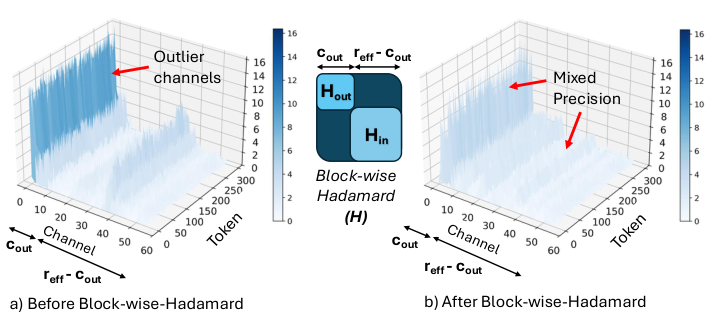
Figure 5. Paper Figure 8, cropped; Bhatnagar et al., CC BY 4.0. The example visualizes a LongChat key head before and after separate Hadamard rotations. The two blocks preserve distinct precision allocations while redistributing magnitude within each block.

The v1 prose near equation (12) contains an inequality saying the outlier rank is much larger than the inlier rank, which conflicts with its stated 20:80 split. The operational description and the later tables consistently allocate 20% to the higher-precision block. This review follows that explicit split rather than propagating the contradictory inequality.

The ablation is informative but not a perfectly isolated comparison at equal precision. At 75% low-rank compression, global Hadamard with uniform three-bit quantization scores 58.23; mixed precision without rotation scores 57.27; the combined block-wise strategy scores 59.18 on the five-task average. The first option has a different average bit budget. The result supports the combined configuration, but does not quantify a pure rotation effect with all other resources held fixed.

6.2 Payload arithmetic versus allocated memory

For a uniform simplified model with $h$ key heads, latent key rank $r_h^K$, joint value rank $R_V$, and common average precision $\bar b$, a more explicit cache expression is

$$M_{\mathrm{latent}}= \frac{BT\bar b}{8} \sum_{\ell=1}^{L} \left(\sum_h r^K_{\ell,h}+R^V_\ell\right) +M_{\mathrm{metadata}}+M_{\mathrm{padding}}. \tag{15}$$

Protected layers should be entered with their actual full widths and precision. Extra factors and temporary workspace belong in total device memory, even though they are not part of the persistent token payload. Rank rounding to a supported kernel tile can also change the achieved ratio.

As an illustrative bound, suppose a 32-layer model leaves three equal-size layers entirely at FP16 and compresses the others to $0.25\times3.2/16=0.05$ of their original payload. The full-cache retained fraction would be

$$f=\frac{3}{32}+\frac{29}{32}\times0.05 =0.1390625, \qquad f^{-1}\approx7.19. \tag{16}$$

This is not a correction to the authors’ measured footprint: the paper does not give enough accounting detail to assume that exact interpretation for every configuration. It is a diagnostic example showing why the meaning of “20× overall KV reduction” must specify whether exempt layers, their quantization, and rank aggregation are included. A theoretical payload multiplier and a measured full-model allocation are different quantities.

Algorithm 2. Consume a compressed cache during decoding

This procedure summarizes the dataflow described in Section 3.3 and Appendix A.6. It is not a new implementation or a claimed reproduction.

1. Project the new hidden state into latent keys and values.
2. Apply the prepared block rotations through the projections.
3. Quantize and append the new latent cache coordinates, if enabled.
4. For each key tile required by the current query:
   a. Read and dequantize the latent coordinates.
   b. Reconstruct key coordinates in the fused computation.
   c. Apply the position-specific RoPE transformation.
   d. Accumulate attention scores without storing a full key cache.
5. Normalize the scores with the attention softmax.
6. Stack head probabilities and multiply by shared latent values.
7. Apply the prepared head-specific value/output factors.
8. Sum the head contributions and continue the decoder block.

The speed depends on keeping the intermediate expansion local to the fused computation. Writing an FP16 full cache to memory after step 4 would give back much of the bandwidth benefit. Similarly, dequantizing the entire latent cache into a separate buffer before use would add avoidable traffic. The paper’s kernel discussion explains these choices at the algorithmic level.

7. What the quality experiments support

7.1 Adaptive allocation is valuable, but preservation is model-dependent

Table 1 reports six-task common-sense accuracy alongside perplexity. On LongChat, the dense average is 61.53; STAR-KV at 60% compression also gives 61.53, while 75% compression gives 60.49. On LLaMA-2-7B, the corresponding averages are 65.05, 64.34, and 62.73. On LLaMA-3-8B-Instruct, they are 67.87, 65.42, and 64.15.

The losses at 75% compression are therefore 1.04, 2.32, and 3.72 percentage points. The first result is impressive for aggressive rank reduction, but the model variation rules out a blanket “no accuracy loss” description. Equal aggregate accuracy at one setting also allows gains on some tasks to offset losses on others.

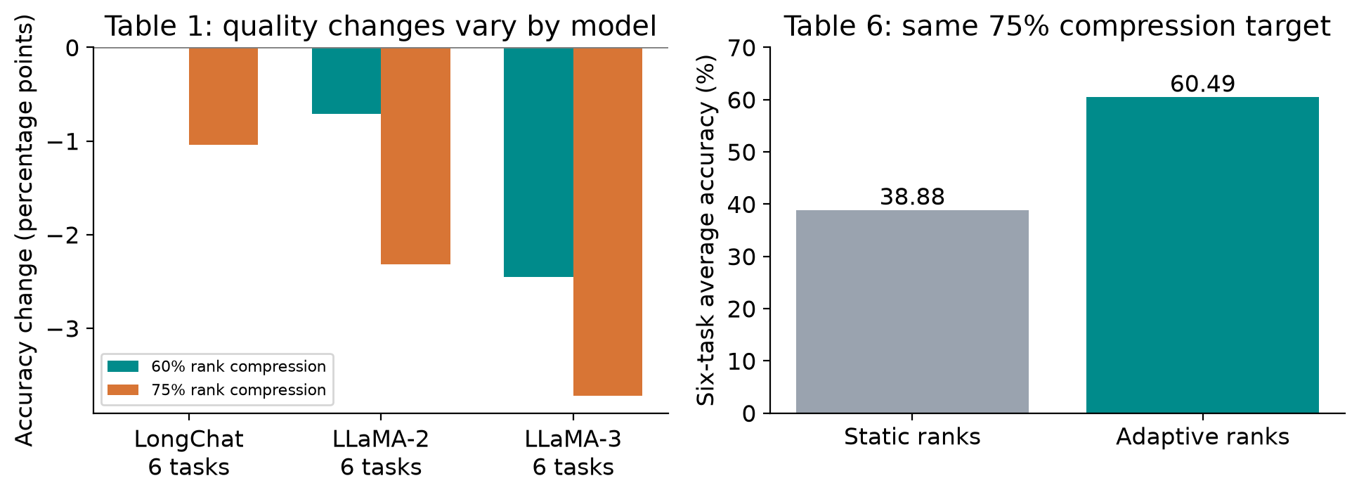
Figure 6. Original redraw from paper Tables 1 and 6. Left: STAR-KV minus dense six-task accuracy, in percentage points. Right: static and adaptive rank selection at the same 75% compression target. Values are transcribed from the paper; no model experiment was run for this review.

The static-rank ablation is strong evidence for allocation quality: at the same 75% target, a uniform rank policy scores 38.88 against 60.49 for STAR-KV. The 21.61-point gap is much larger than the difference between several calibration datasets. It supports the claim that where rank is retained matters greatly. It does not alone identify the contribution of every component, nor does it compare against every possible nonuniform heuristic with matched adaptation effort.

Perplexity and accuracy should also remain distinct. The LongChat WikiText-2 perplexity slightly improves from 6.86 to 6.83 at 60%, while its C4 perplexity changes from 9.93 to 9.98. Such small changes can reflect adaptation and benchmark variation; they do not show that the compressed representation contains exactly the same information. The LLaMA-2 ReCalKV row additionally prints a mean perplexity of 11.32 next to component values 6.75 and 13.63, whose simple mean is 10.19. Because the intended aggregation is not explained, that summary cell is not a reliable basis for a fine-grained comparative claim.

7.2 Long-context evidence is narrower than maximum capacity

On LongChat, LongBench averages are 40.81 for dense and 39.09 for STAR-KV at 60% compression. On LLaMA-3.1-8B, the main table gives 42.23 and 39.58. These are mixed-task averages, not percentages of preserved tokens or probabilities of exact answer equivalence.

RULER at 4K is especially revealing. LongChat changes from 88.80 to 88.26, with another calibration seed reaching 88.71. LLaMA-3.1-8B changes from 96.94 to 89.03. The latter 7.91-point loss is material even though STAR-KV outperforms the shown Palu result. “Better than another compressor” and “close to the dense model” are separate judgments.

Appendix Table 13 extends LongChat RULER to 16K: dense scores 85.69, Palu at 60% scores 62.94, and STAR-KV at 60% scores 84.16. This is useful longer-context evidence, but still not a quality evaluation at every context length supported by the memory experiment. Fitting 128K tokens and correctly using all 128K tokens are different properties.

There is also an internal inconsistency worth preserving. Appendix Table 14 is labeled LLaMA-3.1-8B, yet its STAR-KV 60% row reproduces the LongChat 60% row from main Table 2, including the 39.09 average; the main LLaMA-3.1 row instead averages 39.58. The appendix’s 50% result may be interesting, but this conflicting 60% row should be flagged, not silently reconciled by selecting a preferred value.

7.3 Mixed precision and token eviction

The 3.2-bit table uses five tasks, excluding WinoGrande, and its dense average is 60.34. At 60% and 75% rank compression, the mixed-precision averages are 60.12 and 59.18. These must be compared with 60.34, not the six-task 61.53 used elsewhere. The precision split ablation also shows a trade-off: a 40:60 split scores 59.52 at 3.4 average bits, while the default 20:80 split scores 59.18 at 3.2 bits. The default is a chosen balance, not the highest-accuracy row.

Combining low rank with token eviction acts on two different dimensions. Retaining 40% of channels and 40% of tokens gives an ideal retained fraction of 0.16, or 84% compression. The LongChat combination scores 59.99 versus 59.95 for H2O alone and 61.53 for STAR-KV alone. The 0.04-point difference relative to H2O is very small without uncertainty estimates; the clearer finding is that the combined method reduces more cache while retaining a similar aggregate score in that setup.

8. Speedups: three different comparisons

8.1 Measured attention latency at fixed batch size

The RTX 4090 attention experiment uses LLaMA-2-7B and batch size 16. Appendix Figure 12 reports the following overall attention speedups against PyTorch FP16 SDPA where both methods fit:

Context	STAR-KV, 75% rank compression	With 4-bit cache
8K	2.6×	2.2×
16K	3.3×	3.5×

At 8K, quantization’s overhead outweighs part of its bandwidth saving. At 16K, the balance reverses. A smaller representation can therefore be slower than a less compressed one at a particular sequence length. This crossover is exactly the sort of behavior a compression-only metric cannot predict.

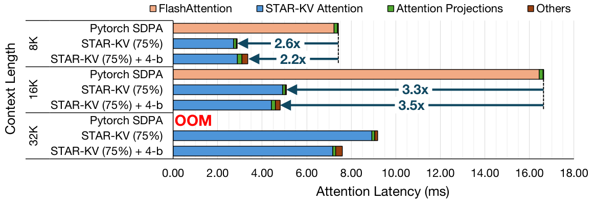
Figure 7. Paper Figure 12, cropped; Bhatnagar et al., CC BY 4.0. All configurations use batch size 16. The dense baseline is out of memory at 32K. The 8K and 16K comparisons are measured; the 32K baseline is unavailable on this device.

At 32K and 64K, the authors extrapolate dense latency linearly from measured 8K and 16K points because the dense cache does not fit. The reported 6.9× at 64K therefore compares a measured compressed runtime with an estimated dense runtime. The result establishes capacity extension and an extrapolation-based performance estimate. It is not a directly measured 6.9× speedup between two runnable configurations on the same hardware.

Even the unquantized 32K number is not identical across the paper: the main text says 4.0×, while the appendix breakdown says 4.1×. These small differences may reflect rounding or measurement scope, but there is no reason to manufacture an explanation. The more useful message is the baseline qualification shared by both figures.

8.2 A larger GPU provides a measured long-context comparison

The RTX PRO 6000 experiment uses a 96 GB device and the same batch size 16. The dense baseline fits throughout the reported range. At 128K, STAR-KV without quantization reaches 2.9× attention speedup and the four-bit variant reaches 4.3×.

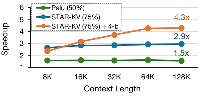
Figure 8. Paper Figure 13, cropped; Bhatnagar et al., CC BY 4.0. On RTX PRO 6000, the dense baseline fits at the shown context lengths. These measurements are attention-operator results on a different GPU, not end-to-end request speedups.

This experiment strengthens the argument that benefits are not solely an artifact of extrapolation. It also illustrates why one should compare like with like: the hardware, context range, and available memory differ from the RTX 4090 experiment. The 4.3× result cannot be substituted into a claim about consumer-GPU end-to-end latency.

8.3 Maximum throughput includes a batch-capacity benefit

Table 5 increases batch size until GPU memory is exhausted for each method. Its generation-throughput results include:

Context	Dense tokens/s (batch)	STAR-KV tokens/s (batch)	Ratio
1K	249.8 (16)	751.0 (128)	3.01×
4K	69.0 (4)	212.2 (32)	3.07×
16K	18.0 (1)	56.6 (8)	3.14×

These are useful capacity-limited serving results. They show that reduced memory permits more concurrent sequences and higher aggregate token production. They do not show a 3.14× decrease in the latency of one sequence: the 16K comparison changes batch size from one to eight. The text separately mentions fitting 128K on a single RTX 4090, while the table’s throughput sweep runs from 1K to 16K. Those claims should remain separate.

A simple Amdahl calculation makes the distinction concrete. If attention occupies fraction $f$ of fixed-workload runtime and is accelerated by $s$, the ideal overall speedup, before new overhead, is

$$S=\frac{1}{(1-f)+f/s}. \tag{17}$$

For an illustrative $f=0.5$ and $s=3.5$, this is about 1.56×. This is not a prediction for the paper’s setup; its actual fraction is not supplied here. It demonstrates why an attention speedup does not transfer directly to whole-model speed, while batch-capacity changes can create a separate throughput benefit.

9. Limitations and failure boundaries

The evidence concentrates on a small set of model families and common-sense, language-modeling, and selected long-context tasks. There are additional Mistral-7B and LLaMA-2-13B results, but this still does not establish preservation for arbitrary architectures, multilingual workloads, tool use, long-form reasoning, or rare exact retrieval. Calibration on educational text is a meaningful distributional choice, not a neutral sample of every future deployment.

Protected layers and weight adaptation complicate attribution. Some quality comes from the learned ranks, some may come from adaptation of the student, and some is protected by excluding sensitive layers. The static-rank ablation is useful, but a deployment reader should still ask whether a competing configuration received equivalent adaptation data, training steps, and protection rules. That comparison determines how much of the advantage belongs specifically to the threshold mechanism.

The compression objective does not directly optimize allocated bytes or hardware time. Rank selection may land on inconvenient tile sizes. A theoretically smaller joint value representation may require larger factors or additional output work. Quantization can improve long-context performance and hurt short-context performance. These boundaries suggest that the final configuration must be selected against the actual quality and latency constraints, not merely the lowest average bit count.

There is no exact equivalence guarantee to the dense model. Rank truncation removes directions, low-bit storage introduces rounding, and model adaptation changes the function. Small average benchmark differences are evidence of empirical tolerance, not a proof of losslessness. Likewise, stable rank profiles across several datasets do not bound failures outside those datasets.

Finally, the paper’s accounting ambiguities limit some headline interpretations: the preparation-cost statements, the exempt-layer denominator for extreme compression, the inconsistent LongBench row, and extrapolated high-context consumer-GPU baselines all deserve explicit qualification. None erases the measured moderate-context or larger-GPU improvements, but each constrains the strongest conclusion one can draw.

10. Critical analysis: what should the optimization target really be?

The most persuasive idea is the separation of representational expressiveness from runtime placement. Joint values preserve cross-head structure while moving reconstruction after aggregation. Head-wise keys reduce the cost that RoPE prevents from being removed offline. This is a more useful general principle than any one retained rank: compression should preserve freedom where algebra makes that freedom cheap to consume.

The least settled part is the relationship between a threshold and a deployment budget. A better formal target would distinguish final cache memory, kernel time, and output distortion. Conceptually, one could pose

$$\begin{aligned} &\min_{\theta,\boldsymbol\alpha}\; \mathbb E_{x\sim\mathcal D} [D_{\mathrm{KL}}(p_T(\cdot\mid x)\|p_{\theta,\boldsymbol\alpha}(\cdot\mid x))] \\ &\quad\text{subject to}\quad M(\boldsymbol r,\boldsymbol b)\leq M_0, \quad t(\boldsymbol r,\boldsymbol b)\leq t_0. \end{aligned} \tag{18}$$

This is an analytical proposal, not the objective evaluated by STAR-KV. The difficulty is that ranks are discrete, runtime depends on hardware shape, and the output loss depends on calibration coverage. A smooth threshold is an effective search tool, but its usefulness does not make the exponential penalty a faithful estimator of either constraint.

A particularly informative next study would hold the final deployed budget fixed while comparing learned thresholds, activation-weighted spectral heuristics, and direct rank search under equal adaptation effort. It should evaluate after hard conversion and after quantization, rather than only during the surrogate phase. That would isolate whether learning improves allocation itself, whether model adaptation compensates for allocation errors, or both.

For system evaluation, two curves are needed. The first holds batch size and context fixed to measure per-step execution efficiency. The second allows batching to vary under a fixed device-memory limit to measure capacity-limited throughput. Both are legitimate. Reporting them separately prevents a user seeking low single-request latency from treating an aggregate throughput gain as a latency guarantee.

The current experiments already contain signs of a multi-objective frontier: higher precision is not always fastest, lower reconstruction error is not always cheapest, and the default precision split is not the highest-accuracy setting. The research opportunity is to make those choices explicit and reproducible as a budgeted policy. The recently queued MetaKV paper addresses configuration selection from a different angle; it is a useful future comparison, not evidence that STAR-KV has already solved that selection problem.

11. Conclusion

STAR-KV demonstrates that fine-grained learned ranks can substantially improve the quality of aggressive low-rank KV compression, and that asymmetric key/value processing can convert part of that compression into measured attention speedups. The method combines offline model adaptation, head-wise keys, joint values, structured quantization, and fused runtime consumption; these components cannot be replaced by a single top-$k$ description.

The strongest defensible summary is conditional: large cache savings and useful speedups are shown on the tested workloads, with meaningful model-dependent quality losses and distinct evaluation settings. The 20× payload claim needs clear accounting, the 6.9× consumer-GPU attention figure uses an estimated baseline, and the roughly 3.1× generation-throughput improvement includes larger batches. Keeping those conditions visible makes the paper more useful, because it shows which part of the design to carry into the next experiment.

References and resources

1. Priyansh Bhatnagar et al. STAR-KV: Low-Rank KV Cache Compression via Soft Thresholding for Adaptive Rank Control, v1, 2026-06-07. Full PDF and HTML. Main Sections 3–5 and Appendices A.1–A.6 support the method and measurements discussed here.
2. Author-provided STAR-KV repository, supplied as a resource entry point.
3. CC BY 4.0, the paper’s license. Figures 2–5 and 7–8 are attributed crops or arrangements; Figures 1 and 6 are explanatory drawings made for this review.