Self-Indexing Attention: One Sign Field for Retrieval and Compression

Review date: 2026-10-28
Paper: Self-Indexing Attention for Compression-Compatible Sparse Long-Context LLM Inference
Authors: Xu Yang, Jiapeng Zhang, Yuxin Chen, Feiqiang Sun, Chengguang Xu, Feng Jin, Zhuo Tang
Version and date: arXiv:2609.13205v2, 2026-10-07
Resources: Paper record · Reviewed PDF · Full text

1. The useful idea is a shared representation

Long-context inference has two related costs. Attention must identify and read useful historical tokens, while the KV cache must retain enough numerical information to reconstruct their keys and values. Sparse attention attacks the first cost; cache compression attacks the second. Combining them is not automatically efficient. A retrieval scheme can introduce another index, require high-precision keys that the compressor has discarded, or make selected-token decoding expensive enough to consume the savings.

Self-Indexing Attention makes a narrower and more interesting proposal: reserve one exact sign bit for every coordinate of a transformed key, and let that same bit serve two purposes. A selector compares it with transformed query signs. After selection, a dequantizer combines it with compressed magnitudes to reconstruct the selected keys. The index is therefore part of the stored key representation rather than a second copy of it. [1, Sections 2–3]

The design has three layers that should be assessed separately. An orthogonal transform preserves uncompressed attention algebraically. A sign-based score and query pooling approximate which tokens matter. Finally, low-bit numerical fields approximate the selected keys and values. Only the first layer is exact. A good explanation must not transfer its exactness to the other two.

The reported results are promising but heterogeneous. On Qwen3.6-35B-A3B, the uncompressed sparse variant obtains a LongBench average of 61.84 against dense attention’s 61.44. The matched six-bit key/value configuration obtains 60.88 against a dense compressed baseline’s 60.91. At the operator level, the reported speedup reaches 6.1× for 64K prefill and 10.3× for 64K decode at batch eight. Whole-model Qwen3.5-9B gains are much smaller: 1.35× in time to first token and 1.23× in steady decode throughput under the reported workload. [1, Tables 1–2, Figure 6]

These numbers support a practical argument about representation reuse, not a claim that binary retrieval exactly recovers dense attention or that every model becomes ten times faster. This review develops the construction, derives what is preserved, and then uses the appendices to examine what remains uncertain. All benchmark measurements below are reported by the authors. Constructed examples, error bounds, memory arithmetic and proposed experiments are explanatory analysis, not new benchmark runs.

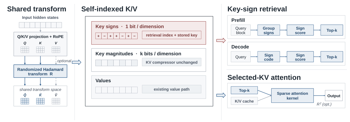
Figure 1: The paper’s Figure 2, cropped from page 3. The sign field is shared by retrieval and compressed-key reconstruction; magnitudes and values remain numerical payloads handled by the selected compressor. Optional value rotation requires a matching inverse transform.

2. Prerequisites: attention, cache traffic and grouping

For one query row, let $q\in\mathbb R^d$ and let $k_i,v_i$ be the historical key and value at token $i$. With a causal candidate set $\mathcal C_t$, dense attention computes

$$\ell_i=\frac{qk_i^\top}{\sqrt d},\qquad p_i=\frac{\exp(\ell_i)}{\sum_{j\in\mathcal C_t}\exp(\ell_j)},\qquad y=\sum_{i\in\mathcal C_t}p_i v_i. \tag{1}$$

The normalization is part of the operation. Dropping a token changes both the omitted contribution and the weights on surviving tokens. A selector that preserves a large fraction of attention mass is useful, but it does not preserve the original output exactly unless the omitted contribution has a special relationship to the retained one.

In prefill, many query rows are processed together. There is substantial matrix multiplication, but the causal attention matrix grows quadratically with sequence length. In decode, one new token extends the context at each step; the historical cache can be much larger than the new query. Repeatedly reading that cache makes bandwidth and memory capacity central constraints. These stages favor different batching and kernel choices even when their mathematical attention operation is the same.

Grouped-query attention, or GQA, maps several query heads to one KV head. If $G=H_q/H_{kv}$, those $G$ heads share historical keys and values but have different queries and attention distributions. Self-Indexing Attention uses that existing sharing structure to amortize retrieval. It does not replace the individual heads’ final attention computation with a single pooled attention output.

Three budgets need distinct names. The storage budget counts all resident key/value payload and metadata. The retrieval budget counts how much of the full history is scanned to propose tokens. The selected-attention budget counts the tokens whose numerical keys and values are decoded and consumed. Reducing the third budget does not remove the first or second. In particular, the proposed method keeps the full compressed history and scans its signs; it is neither permanent token eviction nor constant-time hash-table lookup.

The paper’s quality experiments use approximately 5% attention density, with a minimum selected-token budget of 768 and forced prefix and recent-window tokens. This minimum matters: a nominal budget of 768 is about 4.69% of a 16K history, but 9.375% of an 8K history. These are simple budget calculations, not additional measured operating points. Kernel alignment, overlap between forced regions, and row-wise causal filtering further affect the actual number of historical tokens read.

3. The transform: exact algebra, limited probabilistic implications

3.1 Why rotate after RoPE?

For each layer $l$ and KV head $h$, the paper fixes a randomized Hadamard transform

$$R_{l,h}=D_{l,h}H_{\rm norm},\qquad H_{\rm norm}=\frac{H}{\sqrt d},\qquad D_{l,h}=\operatorname{diag}(\epsilon_1,\ldots,\epsilon_d), \tag{2}$$

where each $\epsilon_j$ is a Rademacher sign. The normalized Hadamard matrix and the diagonal sign matrix are orthogonal, so $RR^\top=I$. The sampled transform is fixed during inference. Query heads sharing a KV head use the same transform; different layer/head pairs receive independently sampled sign patterns. The experiments use a fixed seed of 42. [1, Section 3.1 and Appendix F]

The keys and queries already include rotary positional encoding before this shared transform is applied. The order is important. Attention logits are defined by the RoPE-encoded vectors. Applying an arbitrary rotation before RoPE would generally require a separate commutation argument, which this construction does not need.

Using row vectors, set $Q'=QR$ and $K'=KR$. Then

$$Q'K'^\top=(QR)(KR)^\top =QRR^\top K^\top=QK^\top. \tag{3}$$

Every logit is unchanged in exact arithmetic, so the softmax weights are unchanged too. Values can remain in their original basis. Alternatively, if the cache stores $V'=VR$, then

$$\left[\operatorname{softmax}\!\left(\frac{Q'K'^\top}{\sqrt d}\right)V'\right]R^\top =\operatorname{softmax}\!\left(\frac{QK^\top}{\sqrt d}\right)V. \tag{4}$$

This derivation explains both the optional value transform and the inverse at the output. Omitting the inverse while using transformed values would change the output basis. It also identifies where approximation actually enters: finite precision, sign-based selection and numerical quantization, rather than the intended orthogonal change of coordinates.

3.2 What random signs establish

For fixed vectors $x,y$, a transformed coordinate can be written as $z_j=\sum_a x_a\epsilon_a H_{aj}/\sqrt d$. Since the random signs have zero mean and independent cross-products, direct expansion gives

$$\begin{aligned} \mathbb E[z_j]&=0,\\ \operatorname{Var}(z_j)&=\frac{\|x\|_2^2}{d},\\ \operatorname{Cov}((xR)_j,(yR)_j)&=\frac{x y^\top}{d},\\ \operatorname{Corr}((xR)_j,(yR)_j)&=\frac{x y^\top}{\|x\|_2\|y\|_2}. \end{aligned} \tag{5}$$

The covariance calculation drops terms with different sign indices because their expectation is zero. The remaining diagonal terms use $H_{aj}^2=1$. This connects a coordinate’s correlation across two transformed vectors to their original cosine similarity. It is a useful motivation for comparing signs.

However, the calculation is over transform randomization. A deployed transform is one fixed realization. Its coordinates are not independent Gaussian projections, and the Hadamard family is not a uniformly sampled rotation over all orthogonal matrices. Equal first and second moments do not determine the probability of a sign collision or the rank of all keys under a finite-bit score. This distinction is explicit in the paper and should survive any simplified account of it.

For a truly random isotropic hyperplane, the ideal sign-agreement probability is $1-\theta/\pi$ for angle $\theta$. That formula is a reference model, not a theorem about independent bits in this deployed structured transform. Figure 2 plots the ideal relationship to explain the threshold; it is not a fit to the paper’s measurements and not a top-k recall guarantee.

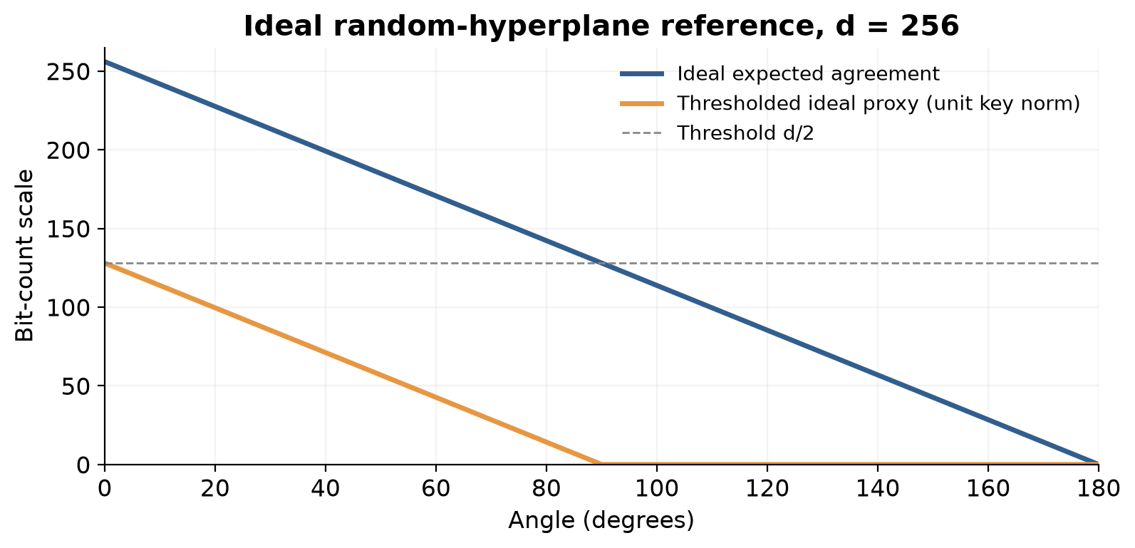
Figure 2: Explanatory plot for ideal random hyperplanes at dimension 256 and unit key norm. It illustrates why agreement above half the coordinates favors acute angles. Structured Hadamard coordinates and pooled queries do not inherit the ideal model’s assumptions automatically.

3.3 Why signs are kept intact

A sign/magnitude representation separates a transformed key into $z_i=s_i\odot m_i$, with $s_i=\operatorname{sign}(z_i)$ and $m_i=|z_i|$. The signs are bit-packed without lossy quantization; an external numerical compressor handles magnitudes and values. The same sign field is read for selection and later used in key reconstruction.

The paper motivates this choice partly through approximately balanced sign bits over transform randomization. That statement does not imply every fixed deployed sign stream has maximum entropy, or that signs are independent across tokens. More importantly, a lossy sign flip has two effects: it changes the reconstructed key and can change a discrete top-k decision. Magnitude noise is also consequential, but it is confined to a different path when the signs used for selection remain exact. [1, Section 3.3]

4. Retrieval: a cheap proxy that still scans history

Let $s^Q$ be the sign vector of a transformed query and $s_i^K$ the stored key signs. The selector counts agreements and restores key magnitude through a norm:

$$a(q,i)=\sum_{j=1}^{d}\mathbf 1[s_j^Q=s_{ij}^K],\qquad \phi(q,i)=\max\{a(q,i)-\tau,0\}\,\|k_i\|_2, \qquad \tau=\frac d2. \tag{6}$$

For the Qwen setting with $d=256$, the threshold is 128. Pure agreement is angular: two keys with equal direction but different norms have the same sign code. Multiplying by the key norm restores one component of the original dot product. For a single query, its norm is constant across keys and need not affect ranking. That observation does not make the entire proxy equal to a dot product, especially after multiple queries have been pooled.

With bit-packed words, agreement can be computed as $d-\operatorname{popcount}(S_Q\oplus S_K)$. Equivalently, one can count positions in which both bits are one and positions in which both are zero. The complement operation must be restricted to valid coordinates in the last packed word. In signed $\{-1,+1\}$ notation, the binary inner product is $2a-d$, so subtracting $d/2$ is proportional to taking the positive part of that binary inner product.

This is attractive because compact signs can be scored with binary matrix operations, avoiding high-precision QK work during proposal generation. Yet a sign score has only $d+1$ possible agreement counts before norm weighting. It throws away within-coordinate magnitude, creates many ties, and maps all below-threshold agreements to zero. The appendix describes deterministic traversal-based tie handling, which makes the operation reproducible but does not make ties informative.

A failure boundary follows immediately. If the useful historical tokens all have low agreement with a pooled sign code, the forced local region may dominate while the long-range portion is determined largely by ties. Increasing the nominal top-k budget can help only to the extent that those tokens eventually enter the selected set. It cannot repair an entirely uninformative ranking at a small budget.

The norm factor is another tradeoff. Without it, retrieval ignores a key’s scale; with it, large-norm keys can outrank better angular matches. The true dot product also depends on norm, so this is not inherently an error. The unresolved issue is whether a coarse, thresholded angle estimate and the norm interact well across all heads, layers and contexts. The paper supplies empirical evidence, not a uniform guarantee.

The word “index” should not be mistaken for sublinear search. Per query group, the method still visits the stored sign field over the relevant history. If a machine word has $w$ bits, a straightforward packed comparison scales as $O(Ld/w)$ word operations, plus norm reads and selection overhead. Hardware binary matrix instructions alter constants and batching efficiency, not the fact that history length still matters. Selected-KV attention then costs roughly $O(kd)$ instead of $O(Ld)$ for each query row. Keeping these terms separate is essential when predicting where the method will pay off.

5. Compression accounting: where the “free” index comes from

After retrieval, only selected entries need their numerical key and value fields decoded. A reconstructed transformed key has the form

$$\widehat z_i^K=s_i^K\odot D_K(c_i^K),\qquad c_i^K=Q_K(m_i^K),\qquad c_i^V=Q_V(v_i). \tag{7}$$

Here $Q_K,D_K$ denote the chosen magnitude encoder and decoder, while $Q_V$ handles values. Normalization conventions may require a stored key norm when reconstructing numerical magnitudes. The important interface is that signs remain directly readable, the selector can access the norm it needs, and numerical fields can be decoded for arbitrary selected tokens.

The paper’s matched comparison requires careful naming. Standalone TQ1 uses one bit for the key and four for the value. “Ours + TQ1” adds an explicit one-bit key sign to a one-bit magnitude field, giving a two-bit full key plus a four-bit value. It should therefore be compared in payload size with TQ2’s two-bit key and four-bit value, not described as identical to standalone TQ1. [1, Appendix F, Table 11]

At $d=256$, the accounting is concrete. TQ2 stores $256\times2/8=64$ bytes of key code and $256\times4/8=128$ bytes of value code. Self-indexing with one-bit magnitudes stores 32 bytes of signs, 32 bytes of magnitudes and 128 bytes of values. Both are 192 payload bytes per token per KV head. Both matched formats additionally store the same four-byte norm, giving 196 bytes before shared quantizer metadata. This arithmetic explains the zero additional index payload claim relative to that particular format.

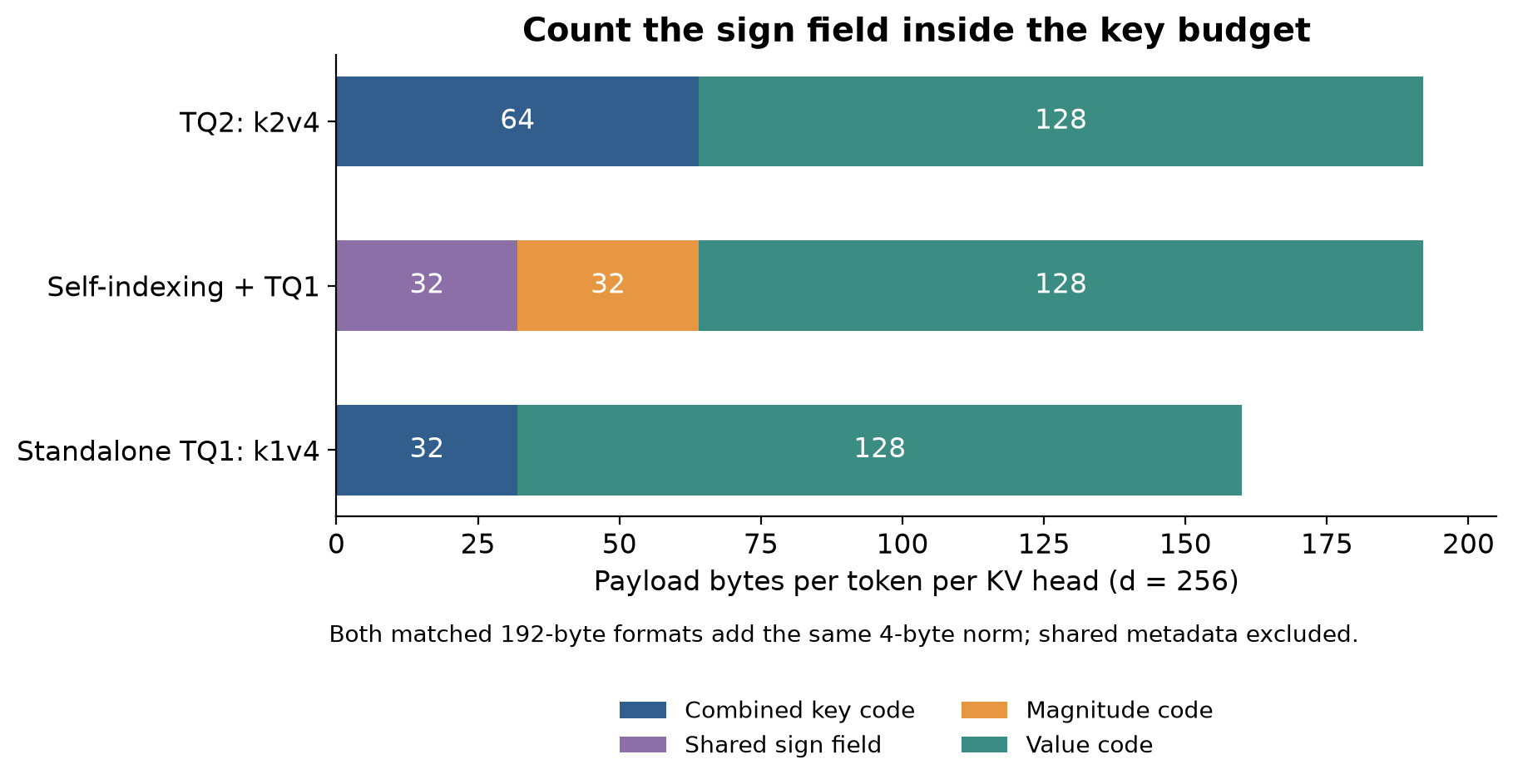
Figure 3: Payload arithmetic from the format definitions in Appendix F, Table 11. The shared sign field is included in the complete key budget. The 192-byte matched formats each add a four-byte norm; shared metadata is excluded. Standalone TQ1 is shown to expose the naming difference, not as a matched storage baseline.

“No additional index metadata” does not mean the cache has no metadata, or that every compressor can accept this layout for free. A codec with inseparable joint key codes, a different rotation, or expensive random-access decoding may not expose the required sign/magnitude interface. Some formats might need repacking or a different numerical quantizer, changing the comparison. The paper’s compatibility claim is strongest for compressors that can preserve the sign field and compress the remaining fields independently.

An alternative would keep a separate binary index alongside an arbitrary compressed cache. That offers more freedom to choose the index representation, but consumes additional bytes and can duplicate information. Another alternative computes retrieval on higher-precision reconstructed keys. It may improve ranking, but then reads or decodes more of the history before knowing which entries are useful. Self-Indexing Attention chooses a constrained common representation to avoid those two costs.

It still retains the compressed full history. The memory advantage is therefore a reduction in bytes per cached token and reuse of an existing field, not removal of all but the selected tokens. This distinction becomes especially important in long-running agents: sparse attention at one step cannot justify discarding an old token permanently if a later query might need it.

6. Sharing proposals without sharing attention outputs

6.1 The reason for absmax-sign pooling

Computing a separate full-history proposal for every prefill query would leave selection expensive. The paper groups 64 query vectors within one KV-head group, pooling across the associated GQA heads and nearby positions. With $G$ query heads per KV head, that corresponds to $64/G$ positions when the grouping divides evenly. Mixing KV heads with different transforms would make their coordinates incompatible, so the group remains within one shared transform.

Mean pooling can cancel informative signs. For coordinate values $+9,-8,+1,-2$, the mean is zero even though one query has a strong positive component. Absmax-sign pooling chooses the sign of the largest-magnitude value in each coordinate:

$$u^*(j)=\arg\max_{u\in\mathcal B}|\widetilde q_{u,j}|, \qquad s^{\mathcal B}_j=\operatorname{sign}(\widetilde q_{u^*(j),j}), \qquad \widetilde q_u=q_uR. \tag{8}$$

The intent is to produce a cheap shared proposal related to keys that matter to at least one query. The motivating ideal would rank a key by $\max_{u\in\mathcal B}q_uk_i^\top$. Absmax-sign pooling is a surrogate for that ideal, not an algebraic evaluation of it. [1, Section 3.4]

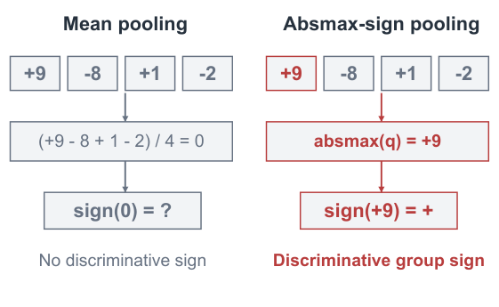
Figure 4: The paper’s Figure 3, cropped from page 5. Absmax-sign pooling preserves the sign of the largest-magnitude coordinate value instead of averaging it away. The chosen coordinate signs may come from different queries.

6.2 A small counterexample to an exact-max interpretation

Consider two already-transformed two-dimensional queries $q_1=(10,-9)$ and $q_2=(-9,10)$. The pooled sign code is $(+,+)$: the first coordinate comes from $q_1$ and the second from $q_2$. Compare equal-norm keys $k_A=(1,1)/\sqrt2$ and $k_B=(1,-1)/\sqrt2$.

The pooled agreement is two for $k_A$ and one for $k_B$. With $\tau=d/2=1$, the thresholded proxy favors $k_A$ and assigns zero to $k_B$. But the maximum actual dot product over the two queries is $1/\sqrt2$ for $k_A$ and $19/\sqrt2$ for $k_B$. A key strongly useful to one query can therefore lose to a key matching the synthetic pooled code.

This constructed example is not a claim about the frequency of such cases in Qwen. It identifies the precise missing guarantee: coordinatewise winners do not necessarily form any real query, and do not preserve the ordering of maximum query–key relevance. The method succeeds only when real query groups have enough compatible structure for the surrogate to be useful. Smaller groups, multiple pooled codes or head-specific proposals are plausible alternatives, but they increase selection work or consume a larger union budget.

6.3 Causality remains a row-wise responsibility

A shared proposal can contain tokens in the future of early rows within the group. Those candidates must be filtered before that row attends. Let $\mathcal I_{\mathcal B}$ be the group’s proposed set, and let $\mathcal L_t$ be the valid recent window for query position $t$. The paper’s row-wise construction can be expressed as

$$\mathcal I_{\mathcal B,t} =\mathcal L_t\;\cup\; \{i\in\mathcal I_{\mathcal B}:i<t-|\mathcal L_t|+1\}. \tag{9}$$

The prefix is included in the proposal; the row’s own local window supplies recent valid tokens. Set union removes overlap. The historical cutoff prevents a shared long-range proposal from duplicating the recent window or introducing future positions. Each query head then computes its own QK scores and softmax over its final valid set.

Filtering can leave fewer than the nominal number of selected tokens, particularly for early rows. Tile alignment may move counts in the other direction. Consequently, an ablation advertised as “same k” should report actual unique causal historical entries after filtering, overlap removal and alignment. The paper’s diagnostic comparison explicitly matches this effective count. A proposal budget and the number of keys a row finally reads are not interchangeable quantities.

7. Two algorithms, one cache interface

The following pseudocode restates the paper’s mathematical data flow. It separates proposal generation from final causal attention and makes the optional value basis explicit. It is not a claim that every kernel has this literal control structure. Prefix and local reservations are counted inside the nominal budget, rather than silently added on top of it.

Algorithm 1. Grouped prefill with a self-indexed cache

Input: RoPE-encoded Q and K; V; per-KV-head transform R;
       budget k; prefix P; recent-window length w.
01. For every KV head, compute transformed keys ZK = K R.
02. Store exact packed signs sign(ZK) and the required key norms.
03. Encode key magnitudes and values with the chosen cache codec.
04. If values use the rotated basis, encode V R instead of V.
05. For each group B of 64 query vectors sharing one KV head:
06.   Transform queries with that head's R.
07.   Pool coordinate signs by absmax across heads and positions.
08.   Scan packed key signs; compute thresholded, norm-weighted scores.
09.   Form a long-range proposal from prefix P and remaining top scores,
      reserving room for each row's recent window within budget k.
10.   For each query row t in B:
11.     Intersect the proposal with valid causal history outside its window.
12.     Union with that row's recent window; remove duplicate indices.
13.     Decode only those numerical K/V entries.
14.     Use the individual transformed query for QK, softmax and value sum.
15.     Apply R-transpose to the output only if values were rotated.
Output: Individual attention outputs plus the full compressed cache.

The cache is constructed for all tokens, whereas selected numerical decoding is row- or group-dependent. Steps 11–12 are semantic requirements, not optional clean-up: they preserve causality and prevent a shared candidate set from being mistaken for an identical row-wise attention mask. Step 14 is also essential. Pooling determines a proposal; it does not replace the true query used by the final attention kernel.

Algorithm 2. Decode with one current GQA group

Input: New RoPE-encoded query heads and key; new value;
       existing full compressed cache; budget k; prefix P; window w.
01. Transform the new key with its fixed KV-head transform R.
02. Append its signs, norm, compressed magnitude and value exactly once.
03. Transform current query heads sharing that KV head with the same R.
04. Absmax-pool those heads into one sign code; do not pool across time.
05. Form the valid forced set F = prefix union current recent window.
06. Score eligible historical signs outside F with the norm-weighted proxy.
07. Select up to k - |F| additional causal indices, respecting alignment.
08. Decode selected numerical keys and values; reuse shared cache reads.
09. For each individual query head, compute its own logits and softmax.
10. Accumulate values and undo the optional value rotation.
Output: Current outputs and the cache extended by one token.

Decode pools the simultaneous heads, not different decoding steps. Otherwise a future query would be unavailable, and a past-query average would answer a different retrieval question. The append operation is shared by all query heads mapped to the KV head; repeating it per query head would incorrectly duplicate the cache.

In both algorithms, short histories require sensible handling when the forced set covers most or all causal tokens. The effective budget cannot exceed the number of available unique tokens. The paper’s minimum budget, tile alignment and recent-window rules are part of the reported configuration; replacing them with an abstract fixed fraction can change both accuracy and runtime.

The paper describes binary matrix operations, fused selection, and selected-KV attention kernels adapted for GQA. These optimizations are important because a theoretically cheap score can still be expensive if it materializes a large score table or requires several extra memory passes. The algorithms above expose that risk without assuming that a bit count alone determines latency. [1, Section 4 and Appendix F]

8. What selection error means for the output

A retained-mass metric becomes more interpretable with a small derivation. Let $\mathcal S$ be a selected set, and let $m=\sum_{i\in\mathcal S}p_i$ be its mass under the original dense softmax. For $0<m<1$, define normalized retained and omitted outputs $y_S$ and $y_R$. If the selected logits and values are otherwise exact, then

$$\begin{aligned} y&=m y_S+(1-m)y_R,\\ y_S-y&=(1-m)(y_S-y_R),\\ \|y_S-y\|_2&\le 2V_{\max}(1-m) \quad\text{if }\|v_i\|_2\le V_{\max}. \end{aligned} \tag{10}$$

The first line partitions the dense weighted sum. The second subtracts it from the sparse output, whose probabilities are renormalized over the retained set. The last applies the triangle inequality and the fact that each normalized weighted average has norm at most $V_{\max}$. At $m=1$, the selection error is zero. The bound is explanatory and can be loose; it does not predict the paper’s normalized RMSE directly.

The derivation shows why both selection and value geometry matter. A small omitted mass is favorable, but even a larger omitted mass can be harmless if omitted and retained values average to nearly the same vector. Conversely, rare tokens with unusual values can matter more than their count suggests. Token recall, retained probability mass and output error are therefore related but distinct measurements.

For quantized selected attention, introduce $y_S$ as the exact selected-set output and $\widehat y_S$ as the actual quantized output. The total error decomposes as

$$\|\widehat y_S-y\|_2 \le \|\widehat y_S-y_S\|_2+\|y_S-y\|_2. \tag{11}$$

The first term includes selected-key logit perturbations and selected-value reconstruction error; the second is selection error. A shared transform can make quantization more benign without fixing a missed token. Better signs can select a useful token without making its compressed value exact. This decomposition is useful when interpreting combined-system results: a single downstream benchmark score does not identify which error component improved.

There is also an interaction absent from the simple bound. In this design, selection reads exact stored signs and norms, while the selected attention kernel uses decoded numerical fields. If a different codec changes the norm convention or the sign extraction basis, the same abstract decomposition no longer isolates an unchanged selector. Compatibility must include those conventions, not just matching the number of bits.

9. Quality results: compare the scope and the payload

9.1 LongBench averages

Table 1 below collects the headline averages from the paper, with scope labels retained because the baselines do not all accelerate the same stage. P denotes prefill, D decode and KV cache compression. [1, Tables 1–2]

Method	Main changed scope	Qwen3.6-35B-A3B	Qwen3.5-9B
Dense	Reference	61.44	56.18
TQ2	KV	60.91	55.92
TQ1	KV, smaller key payload	49.28	49.05
Anchor	P	60.86	55.09
Quest	D	60.87	55.91
SI-KV	D + KV	61.01	56.04
Self-Indexing	P + D	61.84	56.10
Self-Indexing + TQ1	P + D + KV	60.88	56.03

The most defensible summary is that the method preserves broadly comparable aggregate quality in these settings while covering both stages and a compatible compressed cache. The 0.40-point advantage over dense on the larger Qwen model should not be described as a demonstrated accuracy improvement without uncertainty estimates. On the smaller model, the sparse variant is 0.08 points below dense. The direction of a small aggregate difference is less informative than the consistency of the operating point across tasks.

The sharp jump from standalone TQ1 to “Self-Indexing + TQ1” is tempting to attribute entirely to better retrieval. That would be a confounded comparison: the latter has an explicit extra sign bit in its complete key representation. A more appropriate storage-matched reference is TQ2. Against it, the combined method differs by −0.03 points on Qwen3.6 and +0.11 on Qwen3.5. These close averages support the shared-format argument much more directly.

SI-KV is a particularly relevant comparator, but not an earlier name for this paper. The comparison in the paper distinguishes SI-KV’s decode-oriented path, higher-precision query use and its index/key representation from the present method’s binary Q/K retrieval across both prefill and decode with an external numerical compressor. Similar motivation does not make the two methods interchangeable, and their stage coverage must remain visible.

9.2 RULER at longer contexts

The paper evaluates five RULER tasks at 16K, 32K and 64K. At 64K on Qwen3.6, the dense scores for NS3, NM3, CWE, FWE and QA2 are 100, 100, 99.90, 99.33 and 68. Self-Indexing obtains 100, 99, 100, 98.67 and 70; the compressed variant obtains 100, 99, 99.60, 98.67 and 69. The method is near the dense reference on these tasks, including the high-ceiling retrieval tasks. [1, Table 2]

The baseline differences make some tasks more discriminating than others. Quest’s NM3 at this setting is 75 and SI-KV’s is 96, compared with 99 for Self-Indexing. On CWE, SI-KV obtains 92 while Self-Indexing obtains 100. Such per-task gaps are more informative than simply saying that all sparse methods are close on average. However, a near-perfect retrieval benchmark also has little room to reveal small losses; it cannot by itself establish preservation of all long-context abilities.

On Qwen3.5 at 64K, dense CWE is 79.50 and Self-Indexing is 79.90; dense QA2 is 66 and the compressed variant is 64. The compressed variant’s FWE is 96.67 versus dense 100. These differences are modest within the table but matter to a reader deciding whether a particular workload tolerates occasional long-range misses. Aggregate similarity is not a substitute for identifying the task type that the application depends on.

Another generalization boundary is context composition. A synthetic needle or word-aggregation task is not the same distribution as a long agent trajectory with repeatedly revised instructions and many semantically similar records. The paper’s benchmark mix is useful evidence; it is not a proof that the selection heuristic will preserve the newest authoritative version of an instruction in every long conversation.

10. Ablations: a strong mechanism signal from a narrow diagnostic

10.1 Pooling and per-head randomization

The pooling ablation reports output NRMSE of 8.1590% for average pooling without per-head flips, 7.7751% for average pooling with flips, 7.4469% for absmax pooling without flips, and 7.1283% for absmax pooling with flips. Both changes help in this diagnostic, and their combination gives the lowest measured error. [1, Table 3]

The direction of the result is consistent with the mechanism: average pooling can cancel signs, while different head-specific randomizations avoid forcing all heads into the same fixed coordinate pattern. But these four numbers should not be presented as broad statistical validation of either mechanism. The appendix makes clear that the diagnostic uses the same selected query rows from one long prompt. A large number of head/position measurements within that prompt does not create a large independent sample of documents or tasks.

10.2 Forced tokens versus learned relevance in the proxy

The detailed diagnostic uses the longest 2WikiMQA prompt, with 17,113 tokens, 32 query positions in the latter half, ten full-attention layers and all query heads. The nominal budget is 768; the prefix is 64 tokens and the recent window is 64, with local kernel alignment to 128. Historical counts are matched after filtering and deduplication. Anchor is adapted to row-wise top-k for this comparison, with block size 16 and step 8; this is not a direct evaluation of its original threshold rule. [1, Appendix B.1]

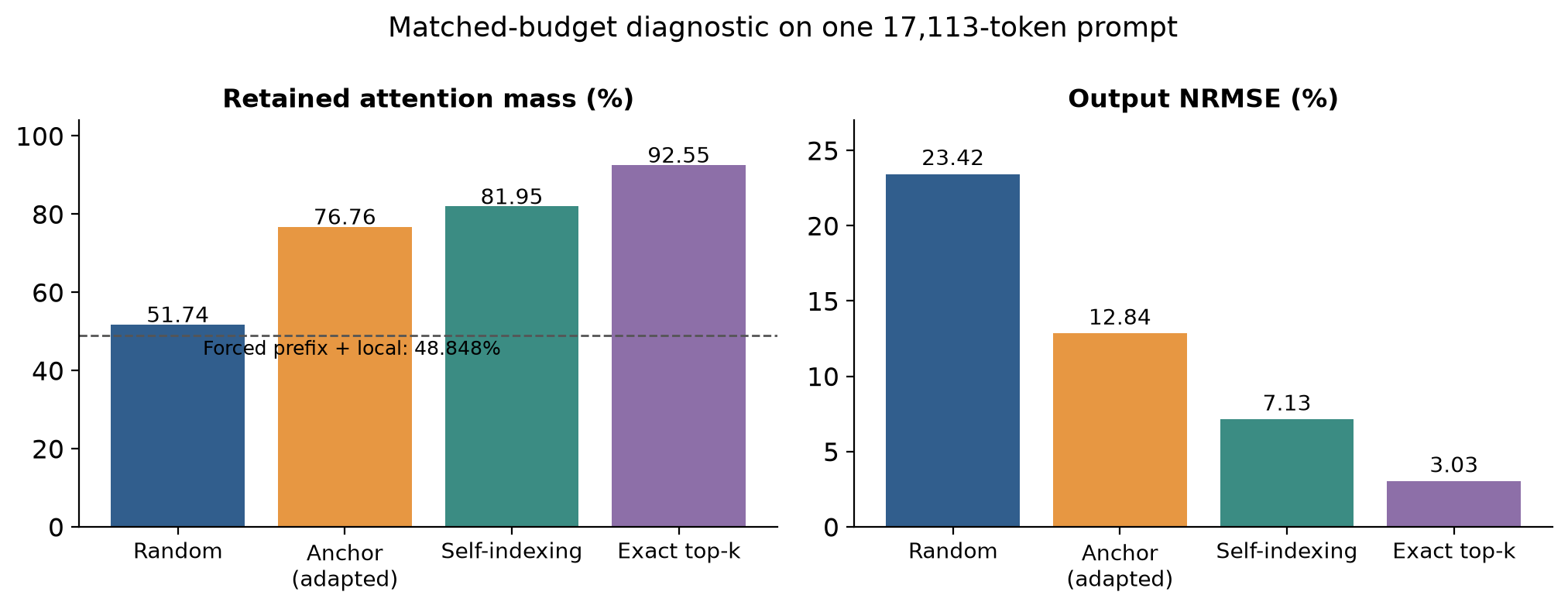
Figure 5: Redrawn from Table 4. The forced prefix and local window already retain 48.848% of attention mass. The rest of each bar measures the contribution of the additional selection, on one prompt rather than a corpus-wide trial. Exact top-k is a diagnostic ceiling, not a low-cost deployment alternative.

Random selection retains 51.739% of mass with 23.4226% output NRMSE. Adapted Anchor retains 76.764% with 12.8360% error. Self-Indexing retains 81.950% with 7.1283% error. Exact top-k retains 92.551% with 3.0253% error. The forced set alone retains 48.848%, so the respective additions beyond it are approximately 2.891, 27.916, 33.102 and 43.703 percentage points.

Subtracting the forced contribution makes two points clear. First, a high retained-mass number does not come entirely from the selector: local and prefix attention already supply a large portion. Second, useful long-range selection still matters substantially. Random selection adds very little, whereas Self-Indexing adds meaningful mass and reduces output error. The gap to exact top-k also remains large enough to motivate better proposal construction.

The error reduction is not proportional to the retained-mass increase. That is expected from Equation (10), because value geometry and renormalization matter. It is also why reporting only token hit rate would be insufficient. A robust evaluation should retain all three views: which tokens were recovered, how much dense probability they carried, and what happened to the output vector and downstream answer.

10.3 Rotation helps quantization too

The transform ablation uses 51,200 keys and 52,633,600 causal QK pairs from the first ten LongBench 2Wiki examples, with unquantized queries and two-bit sign/magnitude keys. Raw keys have key NRMSE 43.79% and QK NRMSE 35.92%. Plain Hadamard gives 34.04% and 20.59%; Gaussian orthogonal rotation gives 34.18% and 20.70%; randomized Hadamard gives 33.06% and 20.07%. [1, Appendix B, Table 7]

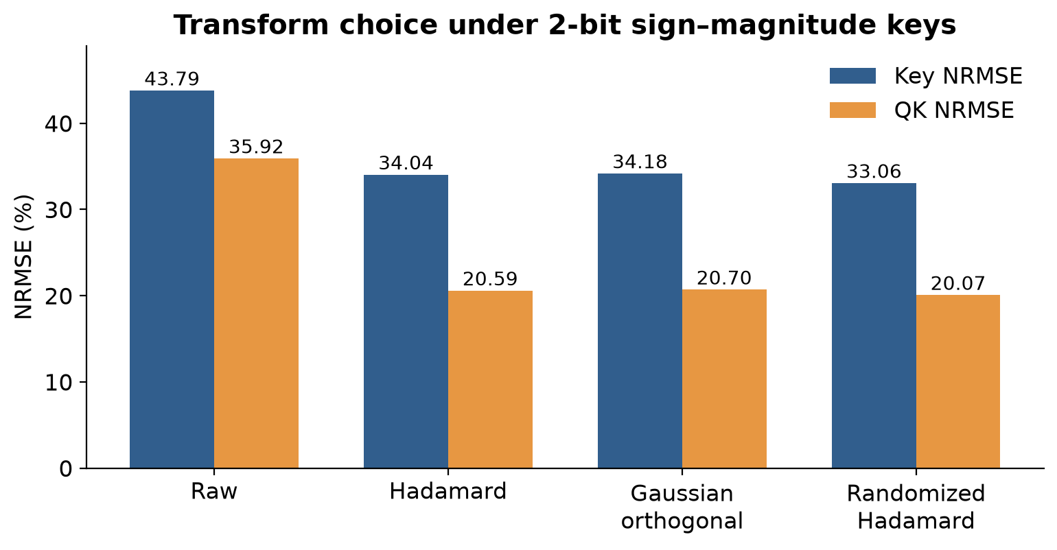
Figure 6: Redrawn from Table 7. These are numerical quantization errors, not downstream task accuracy or selector recall. Queries remain unquantized in this diagnostic, and the key representation uses two bits per coordinate.

Relative to raw keys, randomized Hadamard reduces the reported key error by about 24.5% and QK error by about 44.1%. Relative to plain Hadamard, the reductions are only about 2.9% and 2.5%. Both comparisons are useful, but they answer different questions. Most of the gain comes from moving into a better-conditioned basis; random signs provide a smaller additional improvement in this diagnostic.

The accompanying QK cosine similarities are 0.9545 for raw keys and approximately 0.9817–0.9818 for the three rotations. Similarity at that level does not establish identical token rankings near the top-k boundary. Two nearly equal logits can swap order after a small perturbation. A continuous reconstruction metric and a discrete retrieval decision can therefore behave differently even under the same transform.

11. Efficiency: the selector, the operator and the model

11.1 What the operator timing includes

Figure 7 is valuable because the reported sparse path includes transformation, token selection, selected attention and the optional inverse transform. The comparison is not merely the final small attention multiplication after a free oracle supplies indices. The paper uses BF16 at head dimension 256, FlashAttention-3 for dense prefill and FlashInfer for dense decode. Operator timings use three warm-ups, ten measured repetitions and synchronized median latency. [1, Figure 6 and Appendices C.1, F]

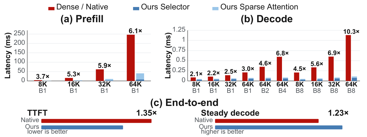
Figure 7: The paper’s Figure 6, cropped from page 9. Panels (a) and (b) are operator comparisons; panel (c) is the whole Qwen3.5-9B model at 64K, batch four and 256 output tokens. The decode metric in panel (c) is throughput, while TTFT is latency.

For batch-one prefill, the speedups are 3.7×, 5.3×, 5.9× and 6.1× at 8K, 16K, 32K and 64K. Batch-one decode gains are 2.1×, 2.2×, 2.5× and 3.0× at the same lengths. At 64K, decode rises to 4.6× at batch two, 6.8× at batch four and 10.3× at batch eight. The batch-eight sequence-length sweep is 4.5×, 5.6×, 6.9× and 10.3×.

This variation is a result, not noise to be hidden behind the largest number. Larger decode batches make full-cache traffic more expensive and improve the opportunity to amortize selection and sparse execution. Prefill has a different balance between matrix throughput, proposal work and cache traffic. Shorter contexts can leave fixed overheads and the minimum token budget relatively more important.

The paper describes an approximately eightfold binary-matrix throughput advantage on its evaluation platform and a large reduction from grouping 64 query vectors. These are ingredients in its selector cost argument. Multiplying ideal instruction throughput by the grouping factor is not a portable whole-system speedup formula: top-k, norms, layout, synchronization, gather and the final attention kernel still take time. Hardware support and the chosen head dimension affect whether the same constants are achievable elsewhere.

11.2 Why the whole-model number is smaller

Qwen3.5-9B has eight full-attention layers out of 32. The remaining layers and non-attention operations are unchanged. Under the reported 64K, batch-four, 256-output-token workload, ten-run mean measurements give 1.35× TTFT and 1.23× steady decode throughput. The 25% fraction of full-attention layers is a layer count, not a measurement that attention consumes exactly 25% of runtime.

If an accelerated component originally occupies runtime fraction $f$ and improves by $s$, an idealized serial cost model gives

$$S_{\rm total}=\frac{1}{(1-f)+f/s}. \tag{12}$$

This follows by normalizing the old total cost to one: unchanged work remains $1-f$, and accelerated work becomes $f/s$. As an illustrative calculation only, $f=0.4$ and $s=6.1$ yield about 1.50× overall. The paper does not report that particular runtime fraction. One cannot infer it from the fraction of full-attention layers or assume that the isolated operator’s speedup applies unchanged inside the complete model.

The same reasoning explains why an apparent 20-fold reduction in attended tokens at 5% density cannot promise a 20-fold model acceleration. The sign scan still touches history, selection costs remain, sparse accesses may be less regular, and unaffected model work sets a floor. The relevant deployment question is whether saved numerical-cache traffic exceeds the entire added selection path at the application’s batch, context and output lengths.

A complete comparison should also distinguish latency-sensitive and throughput-saturated workloads. Higher saturated throughput can come with different queueing behavior. The operator timings and the deployment stress test below answer related but non-identical questions; combining their largest gains into one headline would obscure the actual operating point.

12. DeepSeekV4-Flash: a separate index-cache experiment

12.1 What changes in this integration

The DeepSeekV4-Flash experiment replaces the native FP8 indexer key cache with packed one-bit signs of 128-dimensional transformed indexer keys. It keeps the native model weights, query construction, main KV cache and downstream sparse attention, while retaining top-512 selection. Queries are processed individually in this integration rather than using the Qwen grouping scheme; the agreement threshold is 64. [1, Appendix A and Appendix F]

At the index-key payload level, 128 FP8 coordinates occupy 128 bytes and 128 sign bits occupy 16 bytes, an ideal eightfold reduction in that field. This is not an eightfold reduction of the entire model’s cache or memory footprint. Other KV fields, metadata, weights and runtime buffers remain. The experiment demonstrates a second application of sign-based indexing; it is not the same complete key/magnitude/value format comparison as “Ours + TQ1” on Qwen.

At 64K on LongBench Pro, the reported aggregate for native DeepSeekV4-Flash is 64.1 and the sign-indexed version is 64.2. In the Qwen comparisons shown alongside it, Qwen3.6 changes from 57.5 to 60.5, while Qwen3.5 changes from 33.8 to 33.5. Those aggregate values are useful orientation, but the 128K breakdown is more revealing about the nature of preserved quality.

12.2 An unchanged mean can hide changed capabilities

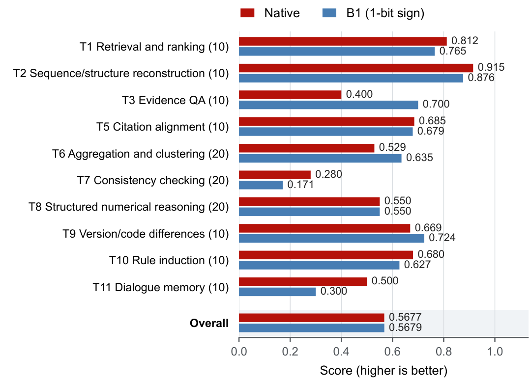
Figure 8: The paper’s Figure 8 from Appendix A, cropped from page 14. This is one LongBench Pro run at 128K. Parentheses show the number of examples per task type. The nearly identical overall means coexist with sizeable gains and losses in individual categories.

The overall values are 0.5677 for native and 0.5679 for the one-bit version. Yet evidence QA changes from 0.400 to 0.700, aggregation from 0.529 to 0.635, consistency checking from 0.280 to 0.171, and dialogue memory from 0.500 to 0.300. Retrieval/ranking moves from 0.812 to 0.765, sequence reconstruction from 0.915 to 0.876, and rule induction from 0.680 to 0.627. Structured numerical reasoning remains 0.550 in this run.

Averaging these changes can support “similar aggregate score in this run.” It cannot support “every capability is preserved.” Several categories contain only ten examples, and the others shown have twenty. With such small groups, changes may reflect substantial sampling variability, genuine task-dependent sensitivity, or both. Paired per-example outcomes and repeated seeds would help distinguish these possibilities.

The AIME 2025 evaluation uses 30 problems over 16 runs, giving 480 sampled answers. Native obtains 234 correct, or 48.75%; the sign-indexed variant obtains 228, or 47.50%. The difference is six sampled answers and 1.25 percentage points. Treating all 480 answers as independent problems would overstate the effective sample size because the same 30 problems recur. Any confidence analysis should preserve that clustering and the paired structure of the comparison.

12.3 Capacity and throughput under 2P1D serving

The deployment stress test uses DeepSeekV4-Flash (0731) on two machines, with two tensor-parallel-four prefill workers and one tensor-parallel-four decode worker. The flood workload contains 144 requests, each with approximately 128K input tokens and 32K output tokens. The relevant comparison uses HiSparse in both configurations. [1, Appendix A, Table 5]

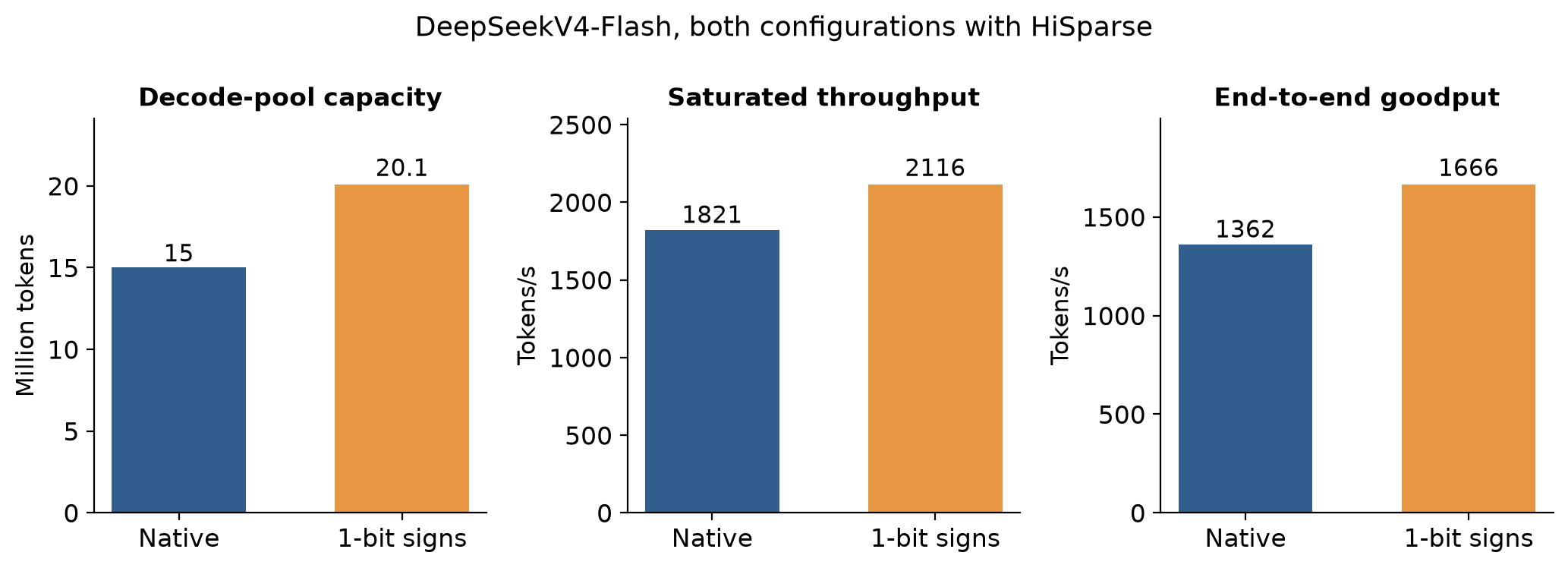
Figure 9: Redrawn from Table 5. Both bars in each pair use HiSparse, so the comparison isolates the reported change from the native indexer cache to one-bit signs within that serving setup. These are deployment results, not isolated attention-kernel timings.

Decode-pool capacity grows from 15.0 million tokens to 20.1 million, approximately 34%. Saturated concurrency rises from 71 to 96, approximately 35%. Throughput increases from 1,821 to 2,116 tokens/s, about 16.2%, and end-to-end goodput rises from 1,362 to 1,666 tokens/s, about 22.3%. Test duration decreases from 56.4 to 46.1 minutes, about 18.3%.

The native configuration without HiSparse has only 5.33 million tokens of decode-pool capacity and fails this flood test. It is evidence of the capacity background, not a valid completed-run denominator for a headline speedup. Comparing the two HiSparse configurations avoids attributing HiSparse’s benefit to the sign representation.

The relationship between memory and throughput is nonlinear. An eightfold reduction in one index field becomes a 34% increase in total pool capacity, then a smaller throughput gain. More resident requests do not automatically translate into equally more tokens per second: compute, communication, scheduling and output generation remain. The paper also acknowledges that a dense compressed-cache baseline can free memory for additional concurrency. Thus capacity gains should be compared against other memory-saving options under the same service constraints, not only against an uncompressed index field.

13. Limitations and failure boundaries

The first limitation is the lossy proposal itself. Sign agreement removes coordinate magnitudes, thresholding removes negative evidence, and pooling merges multiple queries into a synthetic sign pattern. The two-dimensional example demonstrates a real mathematical boundary even if it is not a frequency estimate. Similar failures are plausible when neighboring queries concern distinct entities or when GQA heads have strongly different long-range responsibilities.

The second is that compression compatibility has a contract. The selector requires directly accessible signs, a consistent transformed basis and usable key norms. Arbitrary selected tokens must be decoded efficiently. A format that optimizes sequential cache reads but makes scattered decoding expensive may erase the expected speed benefit. The reported matched representation is convincing evidence for that format, but does not establish universal compatibility with every vector quantizer.

The third is the remaining full-history work. The algorithm compresses the numerical reads used by attention while still scanning signs. As context length grows, that scan, norm traffic and top-k selection remain real costs. Grouping makes prefill cheaper, but does not make its all-history selection work asymptotically linear in the total prompt length. For a fixed group size, the number of groups also grows with the prompt, leaving a quadratic history-scoring structure with a much smaller constant.

The fourth is evidence coverage. The principal Qwen mechanism ablations use a narrow prompt sample; a fixed transform seed and limited model families do not establish invariance across distributions. The paper discusses small variation under other random seeds, but the main tables do not provide the uncertainty information needed to rank small score differences confidently. The 128K DeepSeek task breakdown directly shows why aggregate means alone are insufficient.

The fifth is system portability. Binary-matrix throughput, top-k fusion, tile sizes, the fraction of full-attention work, batching and memory organization all affect the outcome. Head dimension 256 and the reported long-context workloads are favorable, concrete test conditions. Different dimensions, sparse-kernel availability or latency targets can shift the break-even point. “Training-free” describes the absence of model retraining, not the absence of integration work or operating-point selection.

Finally, numerical equivalence is limited to the uncompressed, unselected transform algebra. The actual system deliberately approximates attention. Near-equivalent benchmark scores are useful engineering evidence, but they do not provide an exact-output guarantee for sensitive retrieval, version tracking or long conversational memory.

14. Critical analysis: what would make the claim stronger?

14.1 The real contribution is the interface

The strongest contribution is the observation that retrieval metadata and compressed key data need not be separate objects. Making signs a first-class field creates an interface between a selector and a numerical codec. This is more reusable than a single speedup number, because it suggests a family of selectors and compressors that can share the same cache layout.

The cost of that interface is a constraint on representation. A globally optimal compressor might prefer joint codes that hide individual signs; a better selector might prefer a learned projection or different per-head statistics. The paper chooses a useful common denominator. Future improvements should measure whether the saved index bytes and reads outweigh the accuracy or flexibility lost by fixing that denominator.

This framing also clarifies what should count as progress. A new compressor that reduces magnitude error while preserving the interface is one kind of improvement. A new pooling rule that recovers more attention mass at the same sign-scan cost is another. A serving scheduler that uses the freed capacity effectively is a third. Reporting them separately would make it easier to identify where a combined gain actually comes from.

14.2 A cleaner experiment matrix

A strong follow-up would cross four factors: individual versus pooled queries; plain versus randomized Hadamard; dense versus sign-proposed token sets; and uncompressed versus payload-matched numerical fields. Each cell should retain the same prefix/local policy and report actual unique causal selected counts. This would disentangle the rotation’s quantization benefit from the selector’s ranking quality and the grouping speedup.

The crucial compression control is a fixed complete key/value budget. Comparing standalone one-bit keys with sign-plus-one-bit-magnitude keys is informative about system quality, but not a clean test of selection. Conversely, comparing two selectors at the same nominal k is not clean if one reads more tokens after tile rounding. Byte counts and effective token counts should be first-class experimental columns.

For each cell, I would report retained dense mass, selected-output error, downstream paired scores, selector latency and total operator latency. Exact top-k can remain a quality ceiling even though it is too costly to serve as the claimed fast method. This matrix is a proposed evaluation design, not a set of measurements supplied by the paper.

14.3 Evaluate the tail, not only the average

The 128K task breakdown suggests a specific concern: some applications value consistency checking or dialogue memory more than aggregate QA. A system can preserve the benchmark mean while changing the types of mistakes it makes. I would therefore require task-specific loss thresholds, paired document-level bootstrap intervals and repeated generation runs. The resampling unit should be a problem or document, not every correlated head, position or generated answer.

For retrieval failures, the most revealing slices would contain multiple similar entities, conflicting document versions, delayed corrections and evidence that appears only once far outside the local window. These stress the relationship between grouped proposals and individual query needs. They are more diagnostic than simply increasing sequence length while leaving every retrieval task easy.

One possible adaptation is to use more than one pooled code when group disagreement is high, while keeping a fixed total numerical-attention budget. Another is to reduce the group size for selected heads or layers. Either approach consumes additional selection work and must be judged on a quality–latency frontier. Neither is a free improvement, and neither is established by the reported experiments.

14.4 Make the deployment contract explicit

For a deployable result, I would want a profile that partitions time into transform, sign scan, norm access, top-k, gather/dequantization and selected attention, alongside unchanged model work. The profile should include context and batch sweeps, mixed prompt lengths, cold and warm cache behavior, and the relevant hardware identity. It should also report queueing latency and the precise goodput criterion under a stated service target.

The current end-to-end and 2P1D results already move beyond isolated microbenchmarks. The next step is not merely a larger peak speedup; it is identifying the break-even region where quality constraints and service requirements are met together. That would allow a reader to decide when shared signs are a better use of memory than a different compressor, a larger selected set or a less aggressive grouping policy.

15. Conclusion

Self-Indexing Attention offers a coherent way to combine sparse retrieval and low-bit cache storage. A shared orthogonal basis preserves the uncompressed attention calculation; exact packed key signs then serve both as a compact retrieval representation and as part of the compressed key. Grouped proposals and binary scoring make this representation useful in both prefill and decode, while selected numerical decoding avoids reading the entire full-precision cache.

The important boundaries are equally clear. Structured-transform moments do not prove exact sign-based ranking. Absmax pooling avoids cancellation but can miss a key important to one query. A metadata-free index is relative to a specified sign/magnitude format. Large operator gains become smaller whole-model gains, and similar benchmark averages can hide task-specific losses.

The paper is most valuable as an argument for designing the retrieval representation and cache representation together. Its evidence supports that direction under concrete model and hardware settings. The next questions concern effective token budgets, payload-matched comparisons, task-level failure tails and the complete service cost of turning a compact sign scan into useful attention.

References and figure provenance

1. Xu Yang, Jiapeng Zhang, Yuxin Chen, Feiqiang Sun, Chengguang Xu, Feng Jin, Zhuo Tang. Self-Indexing Attention for Compression-Compatible Sparse Long-Context LLM Inference. arXiv:2609.13205v2, reviewed revision dated 2026-10-07. Main text and Appendices A–G, 23 PDF pages.
2. Full-text version, for navigable equations, tables and appendix context. References to Anchor, Quest, SI-KV, TurboQuant, FlashAttention-3, FlashInfer and HiSparse in this review follow their roles in the reviewed paper; no independent implementation results are asserted.

Figures 1, 4, 7 and 8 are cropped from the paper’s Figures 2, 3, 6 and 8, respectively. Figures 3, 5, 6 and 9 are original redrawings or arithmetic based on its Tables 11, 4, 7 and 5. Figure 2 is an original illustrative plot under an ideal random-hyperplane model. Equations (10)–(12), the pooling counterexample and the proposed follow-up experiments are explanatory analysis by Zhongzhu Zhou.