Self-HPO: When the Harness and the Policy Learn Together

Review date: 2026-10-27
Paper: Self-Evolving Coding Agents via Harness-Policy Optimization
Authors: Zhepei Wei, Wenlin Yao, Baolin Peng, Danqing Wang, Qianhui Wu, Hao Cheng, Yu Meng, Jianfeng Gao
Version and date: arXiv:2610.22791v1, 2026-10-16
Resources: Paper · Full text · Author article · Official code resource · Models

1. The question: what exactly is getting better?

A coding agent can fail after producing a correct edit. It may submit a prose summary instead of a patch, stop with an empty diff, or run out of budget before delivering its work. Conversely, a careful submission protocol cannot manufacture a fix that the model never discovered. These are coupled problems: the surrounding harness determines which situations the model sees, while the model determines whether the harness’s interventions are useful.

Self-HPO makes that coupling an optimization target. It alternates a discrete search over harness changes with reinforcement learning of the policy under the newly selected harness. The current policy also proposes the next harness changes. A better solver can therefore become a better proposer, although the paper’s experiments establish only two rounds of this process, not indefinite improvement.

The strongest result is comparative. In the self-improving setting, the final pair resolves 69.5% of SWE-Bench Verified tasks, against 61.0% for the base agent, 67.5% for policy-only RLVR, and 65.2% for harness-only Self-Harness. Across three benchmarks, the arithmetic mean rises from 57.8% to 64.8%. These are percentages of resolved tasks, averaged across three evaluation runs; the improvement over the base is 7.0 percentage points on that benchmark mean. [1, Table 1]

The important question is not simply whether the joint method wins. It is whether a harness unlocks genuinely useful training trajectories, whether the learned policy remains useful outside its own harness, and how much of the final gain comes from delivery reliability rather than deeper repair ability. The crossed-checkpoint experiment and the appendix’s submission failure make this paper particularly useful for answering those questions.

This review separates three kinds of statement. Numerical results are the authors’ reported measurements. Probability calculations below are explanatory derivations under explicit simplifying assumptions. Proposed controls and follow-up experiments are my analysis; they are not experiments performed by the authors.

2. Prerequisites: policy, harness, trajectory, verifier

The policy is the language model that samples assistant actions. In a terminal agent, an action can include a shell command and the reasoning or text that precedes it. The harness is the program around that model: it builds observations, formats tool results, limits context, recognizes completion, handles errors, and determines whether an attempted final output actually ends the episode. Changing a prompt is one possible harness edit, but changing the termination procedure is another.

Let a task be $x$, the harness be $H$, and the model policy be $P$. A trajectory $\tau$ contains the successive assistant actions and observations. The paper writes the objective as

$$J(H,P)=\mathbb{E}_{x\sim\mathcal D}\, \mathbb{E}_{\tau\sim\pi^{H,P}(\cdot\mid x)}[y(x,\tau)], \tag{1}$$

where $y$ is a binary outcome supplied by an executable verifier. The superscript on $\pi^{H,P}$ matters. A trajectory distribution belongs to the combination of policy and harness, not to the model alone. Identical weights can behave differently when an empty submission is rejected once rather than accepted immediately.

For intuition, factor a trajectory distribution into policy decisions and everything that supplies their context:

$$\pi^{H,P}(\tau\mid x) =\prod_t P(a_t\mid c_t^H)\, K_H(o_{t+1},c_{t+1}^H\mid x,\tau_{\le t},a_t). \tag{2}$$

This is an explanatory factorization, not an additional equation from the paper. $K_H$ includes the environment interaction and harness-dependent context and stopping rules. Some of these transitions are deterministic. The expression explains why updating only $P$ leaves part of the behavior fixed: the model cannot learn from a useful follow-up observation if the harness has already terminated the episode.

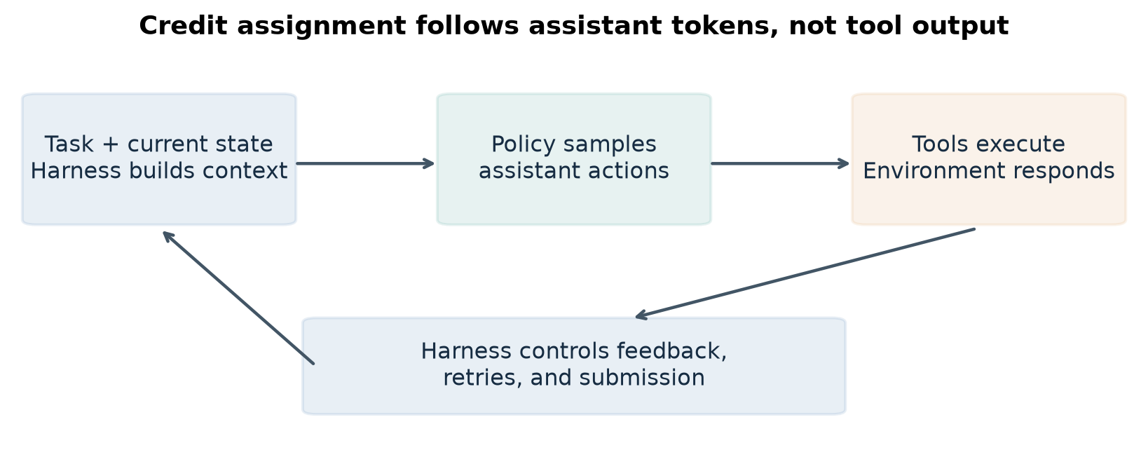
Figure 1. Conceptual reconstruction of the agent loop from Sections 2 and 3 of the paper. Assistant actions are sampled by the policy; observations, feedback, and termination are mediated by the harness. This is an explanatory diagram, not a measured result.

There is also a credit-assignment distinction. A tool may return hundreds of lines, but those lines are not tokens selected by the policy. The training loss should act on assistant-generated tokens rather than treating tool output as model behavior. Yet tool output changes the next assistant distribution. This makes the harness part of the learning environment even when the optimizer never differentiates through it.

Finally, a verifier’s success event is specific. Passing a software repair benchmark requires an acceptable delivered artifact that passes the benchmark’s tests. It is not a direct measurement of every property a developer cares about: maintainability, security, readability, or the absence of untested regressions. A method can improve the measured event by solving more problems, by delivering solutions more reliably, or by both routes.

3. Alternating updates instead of a single giant search

Self-HPO holds one component fixed while updating the other. During the H-step, the current policy proposes and evaluates harness candidates. During the P-step, the chosen harness is frozen and the policy is trained with RL. The improved policy becomes both solver and proposer for the next H-step. The search tasks are also refreshed from failures observed during the preceding P-step. [1, Section 2]

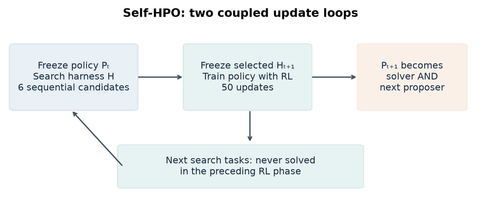
Figure 2. Self-HPO’s two update loops, redrawn from the paper’s method and Algorithm 1. The reported experiments use six harness candidates per H-step and fifty policy updates per P-step, for two rounds.

This resembles coordinate optimization, but the analogy has limits. Harness search is a small, stochastic, discrete proposal process. The policy update optimizes a sampled surrogate objective. The search task distribution changes between rounds. Consequently, neither a global optimum nor monotonic improvement on an unseen benchmark follows from the structure of the algorithm.

The design is nevertheless practical. Holding the policy fixed within an H-step makes candidate comparisons easier to interpret. Holding the harness fixed within a P-step avoids changing the interface during that phase’s learning. The alternative—allowing both to change after every trajectory—could adapt faster, but would make failure attribution much harder. Was a failed rollout caused by a bad repair decision, an incompatible new prompt, or a new stopping rule? Alternation reduces this ambiguity without eliminating the coupling across phases.

The starting search set contains 300 tasks sampled uniformly from the 2,484-task training pool. Later search sets contain tasks that were never resolved during the preceding policy-training phase. Importantly, the next H-step re-evaluates the current pair on those tasks. The method reuses the identities of hard tasks, rather than assuming that old trajectories remain a faithful description of the newly trained policy.

4. The H-step: learning from failures without updating weights

The search evaluates the incoming harness first and keeps it as the incumbent. It then generates six candidates sequentially. A proposal is based on the current best harness and an experience collection containing evaluated harnesses and their trajectories. Each candidate is evaluated on the same search set using the same fixed solver policy. A candidate replaces the incumbent only if its measured resolve rate is strictly greater. Failed candidates still contribute evidence to the experience collection. [1, Algorithm 1]

Algorithm 1. One harness-search phase

Input: harness H, policy P, search tasks S, budget K = 6
1. Evaluate (H, P) on S; store score v and trajectories T.
2. Set best = H, best_score = v, experience = {(H, T)}.
3. For k = 1, ..., K:
4.     Ask P to diagnose experience and propose a revision of best.
5.     Evaluate candidate with the same P on the same S.
6.     Add candidate and its trajectories to experience.
7.     If candidate_score > best_score:
8.         Replace best and best_score with the candidate results.
9. Return best, preserving the incoming harness if no score improves.

The fixed search set is an important local control. Comparing candidate A on one collection of tasks with candidate B on another would mix harness quality with task difficulty. Including the original harness also provides a measured fallback. However, each task receives one rollout for a candidate, so the selected winner can still reflect sampling noise. A strict improvement in the search score is not a significance test and does not guarantee a held-out improvement.

The proposal instructions constrain the edit space. In the supplied prompt, the proposer is asked to retain parent methods and add exactly one mechanism, while preserving model identity, sampling parameters, step and token budgets, and verification rules. This helps keep a change interpretable: it should not win merely by silently granting the agent more inference budget. It also biases the search toward accumulating controls, a choice that can become costly over many rounds.

There is privileged training evidence here. During failure diagnosis, the proposer can inspect reference fixes, while the instructions prohibit embedding those fixes or task-specific facts into the resulting general harness. The relevant distinction is between learning a general mechanism from training evidence and carrying a particular task’s answer into deployment. The paper’s process is therefore not a zero-data procedure. Its credibility depends on task separation and on the generality of the mechanisms, not on the absence of supervised information.

A plausible alternative is to use an external, stronger proposer. The paper evaluates that alternative as HPO, with Opus 4.8 proposing harnesses. Self-HPO’s appeal is that the target policy supplies its own proposals and improves through RL. This avoids requiring that external proposer, but it does not remove the need for a capable initial model, training tasks, a verifier, or a substantial rollout budget.

5. The P-step: why the new harness changes the learning problem

After harness selection, the policy trains on fresh on-policy trajectories under that fixed harness. This is not merely training on better-looking transcripts from a previous agent. A changed termination rule can expose a recovery action that was previously absent from the sampled experience. Successful recovery then becomes part of the policy’s own reward-bearing trajectory.

The paper combines GRPO with Balanced Adaptive Rollout (BAR) from Orchard. The appendix specifies eight sampled trajectories per task before selecting four with a success ratio between 0.25 and 0.75. Additional task sampling continues until 32 valid groups have been collected, giving 128 accepted trajectories in an update. This is a count of trajectories used for training, not the number generated: rejected groups and the extra samples used to form a selected group cost computation too. [1, Appendix A]

The actor objective averages over assistant-token positions. With $\mathcal A(\tau_i)$ denoting those positions, a compact restatement is

$$\mathcal L(\theta)=-\mathbb E_i\left[ \frac{1}{|\mathcal A(\tau_i)|} \sum_{u\in\mathcal A(\tau_i)} \min\left(\rho_{i,u}(\theta)\widehat A_i, \operatorname{clip}(\rho_{i,u}(\theta),0.8,1.28)\widehat A_i\right) \right]. \tag{3}$$

Here $\rho$ compares the current probability of an assistant token with its probability under the rollout policy. The bounds reflect the appendix’s lower clipping parameter 0.2 and upper parameter 0.28. The formula above describes the actor surrogate; the reported optimizer also uses an entropy coefficient of $10^{-4}$ and no KL penalty. It should not be read as a complete specification of every training-system operation.

To understand the clipping, first suppose the advantage is positive. Increasing the token ratio improves the unclipped objective, but the minimum prevents further surrogate gain once the ratio exceeds 1.28. Next suppose the advantage is negative. Decreasing the ratio would improve the objective, but below 0.8 the clipped negative term prevents further gain. The clipping thus limits the incentive for a large update in the favorable direction. It does not constrain the entire new policy to lie in a hard trust region.

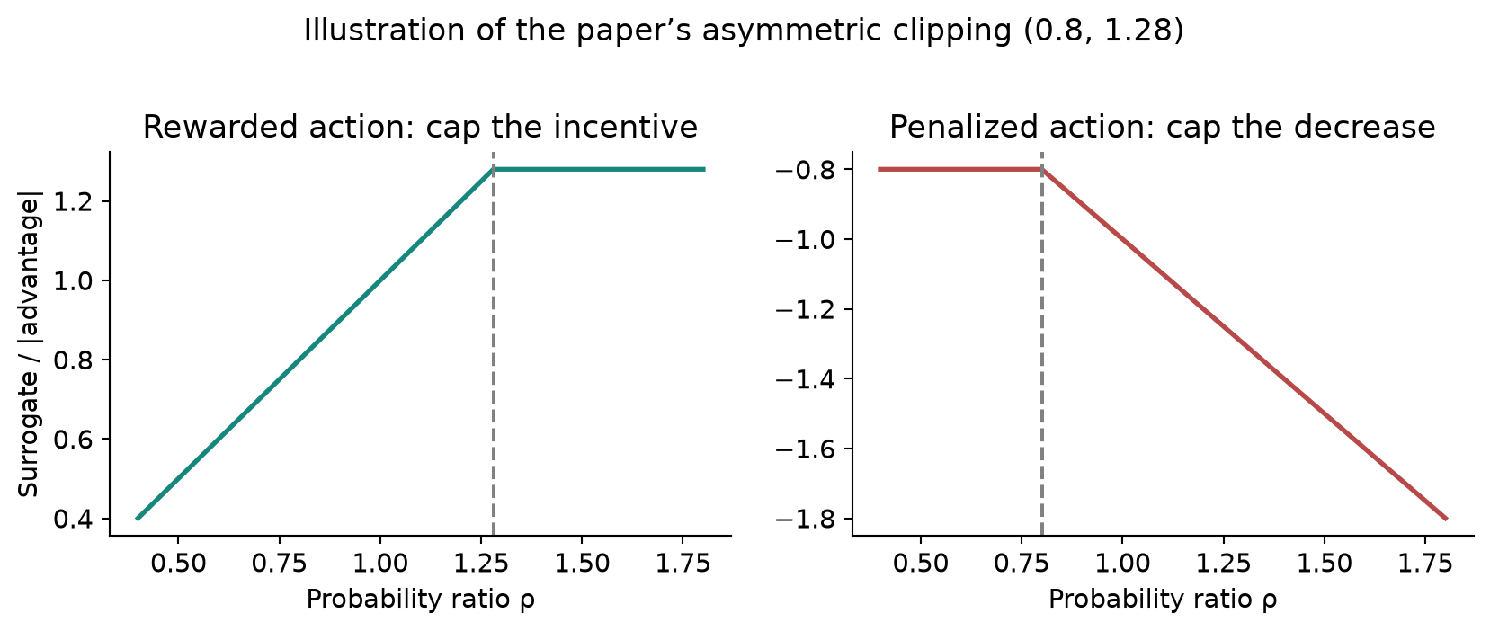
Figure 3. Analytical illustration of Equation (3), using advantage +1 on the left and −1 on the right. The curves are calculated from the surrogate, not measured training behavior. The ordinate is the maximized surrogate; the loss takes its negative.

Length normalization is another design choice with consequences. The factor $1/|\mathcal A(\tau_i)|$ gives an average token contribution per trajectory. Without it, a long episode could contribute more total weight simply because it contains more assistant tokens. But outcome rewards still assign the same trajectory-level advantage to many decisions. A useful final patch does not tell the optimizer which earlier exploration step was unnecessary. Harness changes can make the path easier to learn, but they do not solve temporal credit assignment by themselves.

6. Deriving the learning signal under binary rewards

Consider a group of $G$ trajectories for one task with rewards $r_i\in\{0,1\}$. As background for group-relative learning, define the empirical success fraction $p=G^{-1}\sum_i r_i$. With population-style normalization and ignoring a numerical epsilon, the variance is

$$\frac{1}{G}\sum_i(r_i-p)^2 =p(1-p)^2+(1-p)p^2=p(1-p). \tag{4}$$

The normalized advantage for a success is then $(1-p)/\sqrt{p(1-p)}=\sqrt{(1-p)/p}$; for a failure it is $-p/\sqrt{p(1-p)}=-\sqrt{p/(1-p)}$. These expressions are an explanatory derivation of a common group-relative construction. They are not a claim about an otherwise unspecified variance convention in the paper.

The degenerate cases are the central issue. If all outcomes are zero or all are one, centering gives no within-group reward contrast. A difficult task can consume many tokens while offering no direct group-relative distinction between its sampled trajectories. A harness that turns one failed delivery into one success may therefore improve both the final task outcome and the availability of a training signal.

Under an illustrative IID Bernoulli model with per-rollout success probability $p$, the chance that a group contains both outcomes is

$$\Pr(\text{mixed group of }G)=1-p^G-(1-p)^G. \tag{5}$$

For $p=0.1$, four independent samples produce a mixed group with probability 0.3438. Eight produce at least one success and one failure with probability approximately 0.5695. If eight samples contain both outcomes, a four-trajectory subset with one to three successes can be formed. That is why drawing a larger pool before selecting a group can help. It is not free: samples are paid for before the accepted subset is chosen.

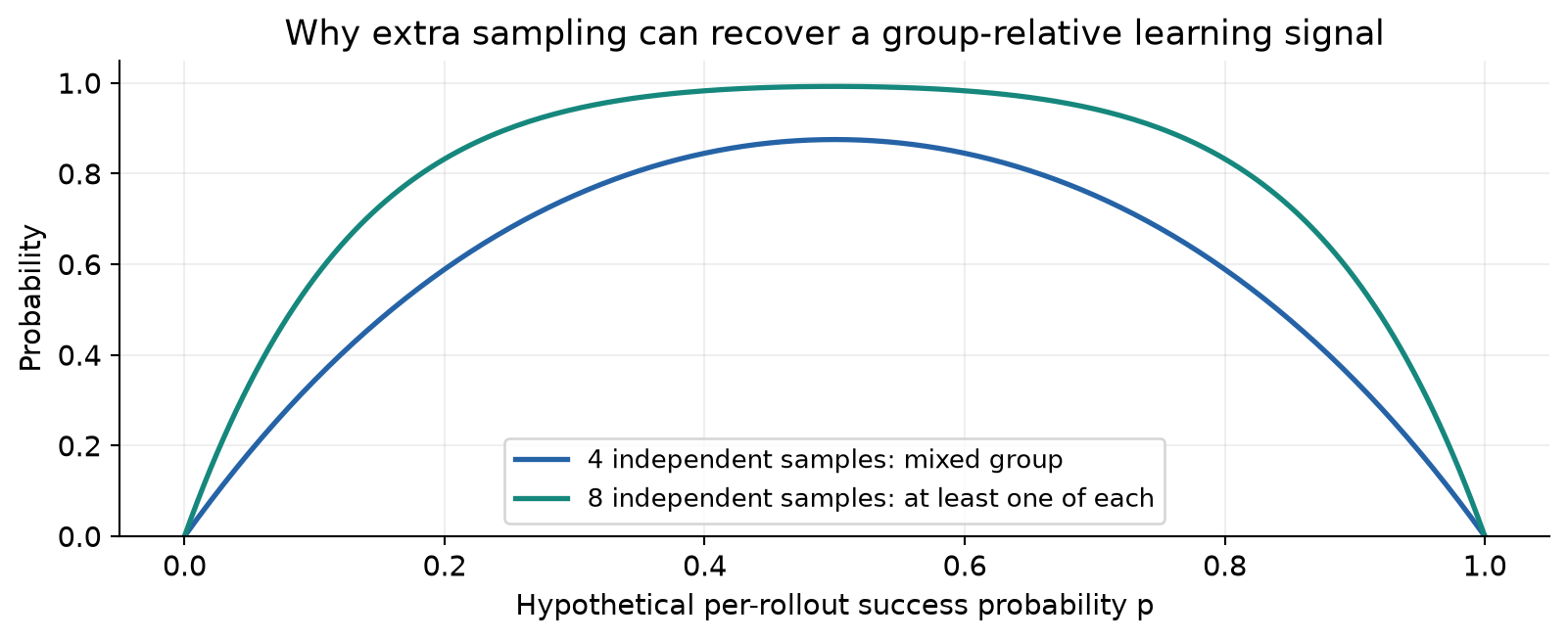
Figure 4. Equation (5) evaluated for four and eight IID attempts. This is a pedagogical probability model, not a measurement of BAR or a prediction for correlated coding-agent rollouts.

Actual trajectories need not be independent or equally likely to succeed, and adaptive sampling changes which tasks contribute to an update. The curve therefore explains a mechanism, rather than estimating the paper’s actual sampling cost. To judge efficiency, one would need the number and length of generated rollouts, their acceptance rates, and the distribution of those quantities over tasks and training time.

7. The moving search set is a curriculum with a specific bias

The next harness search focuses on tasks never resolved in the preceding P-step. This is stronger than selecting tasks the final policy fails on once. A task leaves the never-solved set if any sampled training trajectory succeeded during that phase, even if the final policy is still unreliable on it. The selection therefore emphasizes absence of observed success, rather than low final-checkpoint accuracy.

Under a second explanatory IID model, a task with success probability $p_x$ that receives $m_x$ attempts remains in this set with probability

$$\Pr(x\text{ remains never-solved})=(1-p_x)^{m_x}. \tag{6}$$

This derivation is elementary but useful. Every failed attempt multiplies the survival probability by $1-p_x$. Thus membership reflects both difficulty and exposure. A task sampled twice and one sampled twenty times are not equally strong evidence of a persistent failure mode. During real training, $p_x$ changes with the policy, making a product of time-dependent failure probabilities a more realistic abstraction; the simple formula is only intuition.

The authors’ motivation is sensible: once the policy improves, old failures may be poor targets for the next harness edit. However, the rule can miss a task with one lucky success and frequent subsequent failures. It can also concentrate search on tasks beyond the current policy’s reach. A useful future comparison would keep separate strata for never-solved tasks, unstable low-success tasks, and already-reliable tasks whose regressions should be prevented. That is a proposed alternative, not part of the reported method.

Algorithm 2. Two rounds of coupled training

Input: H0, P0, training pool D with 2,484 tasks
1. Sample S0: 300 training tasks uniformly.
2. For t = 0, 1:
3.     H[t+1] = Algorithm 1(H[t], P[t], S[t], K=6).
4.     Freeze H[t+1] for this policy-training phase.
5.     Collect on-policy trajectories with binary verification.
6.     Form reward-balanced groups and run 50 policy updates.
7.     Retain task identities never solved in this phase as S[t+1].
8.     Use updated P[t+1] as both solver and next proposer.
9. Evaluate the final pair H2, P2 on held-out benchmarks.

The paper describes stabilization of the hard-task set as its stopping consideration and performs two rounds. Stabilization should not be mistaken for proof that further training cannot help. It can also occur when the search space is too restrictive, exploration is inadequate, or the verifier supplies little useful variation. Reporting changes in set membership, not just its size, would help distinguish these explanations.

8. Experimental design: what is held fixed and what is measured

All principal experiments use Qwen3.5-35B-A3B as the base policy and mini-SWE-agent as the seed harness. The 2,484 training tasks come from Python projects in SWE-rebench, SWE-rebench V2, and Scale-SWE. The same pool supports harness search and policy training. The benchmarks are SWE-Bench Verified with 500 tasks, SWE-Bench Multilingual with 300 tasks across nine non-Python languages, and the public V2 split of SWE-Bench Pro with 642 tasks. [1, Section 3.1]

The training setup reported in Appendix A uses a node with eight B200 GPUs, slime for training, and SGLang for serving. Each P-step has fifty updates, giving one hundred in total. Each update uses 32 groups of four accepted trajectories, one epoch, and a global batch of 128. Adam uses a constant learning rate of $10^{-6}$ and weight decay 0.01. Both temperature and top-p are 0.95, and the evaluation step limit is 250. These are paper-reported settings, not measurements made for this review.

The external SFT comparison uses successful Opus 4.8 trajectories from the same training tasks, with two epochs, batch size 64, learning rate $5\times10^{-6}$, and 10% warmup. Sharing tasks does not imply matching every cost: collecting external-model demonstrations, searching harnesses, and sampling on-policy groups have different resource requirements. A fixed number of optimizer steps is only one axis of comparability.

The headline metric is avg@3: the mean resolve rate over three evaluation runs, with a standard deviation. It is not pass@3 and does not mean the system may choose the best of three attempts for each task. When the table reports an overall average, it takes the arithmetic mean of the three benchmark percentages. It does not pool all 1,442 tasks into one weighted rate.

For example, the reported Self-HPO mean is $(69.5+59.7+65.2)/3=64.8$. A pooled rate would give more weight to Pro because it contains more tasks. Neither convention is inherently wrong, but they answer different questions. Equal benchmark weighting is a choice about how much each evaluation domain matters.

The paper reruns environment or API failures. That is reasonable for separating infrastructure accidents from agent quality, but the rerun rule is part of the measurement procedure. A deployment-oriented evaluation should also report operational failure frequency and latency. An agent may have a strong conditional resolve rate while still being expensive or fragile under real service conditions.

9. Main results: two kinds of optimization are complementary

The following table reproduces the mean percentages from Table 1. The source also reports standard deviations; the table here keeps means alone to make the pattern readable. The original source should be consulted for uncertainty on any particular comparison.

Method	Verified	Multi	Pro	Mean
Base	61.0	54.2	58.3	57.8
External SFT	65.0	49.6	49.1	54.6
Meta-Harness	69.1	56.5	64.8	63.5
External HPO	71.6	61.4	66.0	66.3
RLVR	67.5	56.3	61.8	61.9
Self-Harness	65.2	54.3	60.7	60.1
Self-HPO	69.5	59.7	65.2	64.8

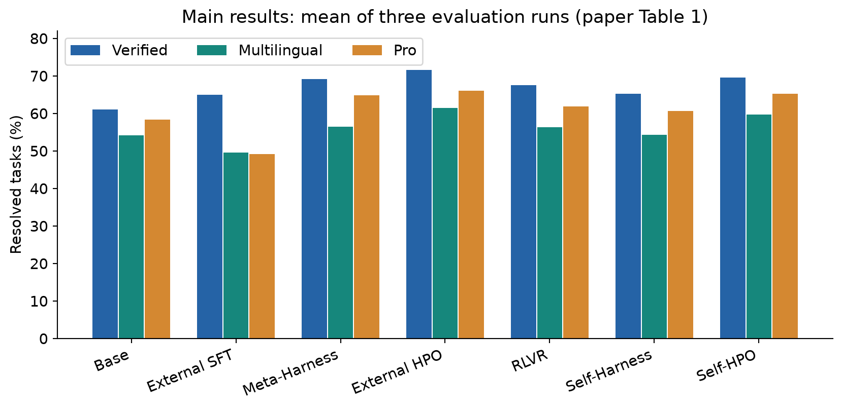
Figure 5. Means transcribed from paper Table 1; no new experiment is represented. The three bars for a method are different benchmarks, not repeated runs. Error bars are omitted here, so bar separation alone should not be interpreted as a significance test.

Within the self-improving setting, Self-HPO beats both component-only baselines on all three benchmarks. Relative to RLVR, the gains are 2.0 points on Verified, 3.4 on Multilingual, and 3.4 on Pro. Relative to the base, the out-of-distribution gains are 5.5 and 6.9 points. These comparisons support a benefit beyond merely improving the original Python benchmark.

The external-model setting reaches a higher ceiling: external HPO scores 71.6 on Verified and 66.3 on the three-benchmark mean. Self-HPO is lower by 2.1 and 1.5 points respectively. The defensible claim is therefore that an external proposer is not required for meaningful joint gains, not that self-proposal has matched or surpassed the stronger proposer.

SFT is an instructive counterexample to a simple “stronger teacher always helps everywhere” story. It improves Verified by 4.0 points but loses 4.6 on Multilingual and 9.2 on Pro relative to the base. Its mean is 3.2 points lower. This shows a generalization problem for this particular SFT setup. It does not establish that supervised learning is universally inferior, since demonstration selection, mixing, objectives, and training budgets can all affect transfer.

The paper reports Self-HPO’s Verified result as $69.5\pm0.9$ and the benchmark mean as $64.8\pm0.6$. These spreads characterize the reported evaluation runs. They are not confidence intervals and do not by themselves measure sensitivity to independent retraining, harness-search randomness, or task-split choice. The direction of the evidence is clear; the full uncertainty of the training procedure is less completely characterized.

10. Crossed checkpoints: complementarity without universal portability

The most revealing experiment evaluates three harness checkpoints with three policy checkpoints on Verified. Rows change the harness; columns change the policy. This separates the value of a component from the value of its native pairing. [1, Table 3]

Harness / Policy	$P_0$	$P_1$	$P_2$
$H_0$	61.0	61.7	64.4
$H_1$	64.3	67.8	68.1
$H_2$	64.5	68.6	69.5

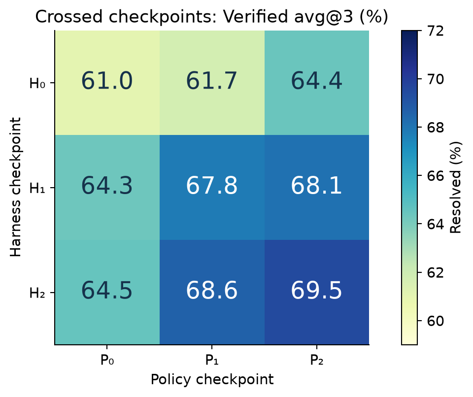
Figure 6. Verified avg@3 means from paper Table 3. Both evolved components retain some value when paired with the initial counterpart, while their final combination scores highest in this matrix.

Start at 61.0. Replacing only the harness with the jointly evolved $H_2$ produces 64.5, a 3.5-point gain. Replacing only the policy with $P_2$ produces 64.4, a 3.4-point gain. Replacing both produces 69.5, an 8.5-point gain. A difference-in-differences contrast is

$$\begin{aligned} \Delta_{\mathrm{interaction}} &=J(H_2,P_2)-J(H_2,P_0)\\ &\quad-J(H_0,P_2)+J(H_0,P_0)\\ &=69.5-64.5-64.4+61.0=1.6\text{ points}. \end{aligned} \tag{7}$$

This is a descriptive interaction contrast calculated from the authors’ table. It says that the joint gain exceeds the sum of the two separately measured gains in these pairings. It does not prove a statistically significant interaction, and it is not a randomized causal estimate independent of the search and training history.

Two numbers must not be silently substituted. The 64.5 obtained by pairing jointly evolved $H_2$ with $P_0$ is not the 65.2 of the independently optimized Self-Harness baseline. Likewise, the 64.4 of $P_2$ under $H_0$ is not the 67.5 achieved by independently training RLVR under the seed harness. The two training paths produce different components. Table 3 tests component carryover; Table 1 tests alternative optimization strategies.

This distinction changes the interpretation. The joint policy is better than the initial policy even under the original harness, so its gains are not entirely locked to $H_2$. Yet it is worse there than the independently trained RLVR policy. Joint learning has yielded a strong pair, not a policy shown to dominate every alternative under every interface.

The intermediate path is also informative: $(H_1,P_0)$ reaches 64.3; training yields $(H_1,P_1)$ at 67.8; another harness step yields $(H_2,P_1)$ at 68.6; and the final policy step reaches 69.5. These are successively smaller increments on Verified. Two rounds demonstrate continued improvement, but they provide too little evidence to extrapolate a long-run scaling law or an unbounded self-improvement trajectory.

11. Ablations: read the reference configuration carefully

The ablation table uses the external-proposer HPO result of 71.6 as its reference. Replacing its policy step with SFT yields 67.2; replacing it with rejection-sampling fine-tuning on the target policy’s own successful trajectories yields 70.5. Keeping the initial search set fixed yields 70.1. Replacing the external proposer with the current policy yields Self-HPO at 69.5. [1, Table 2]

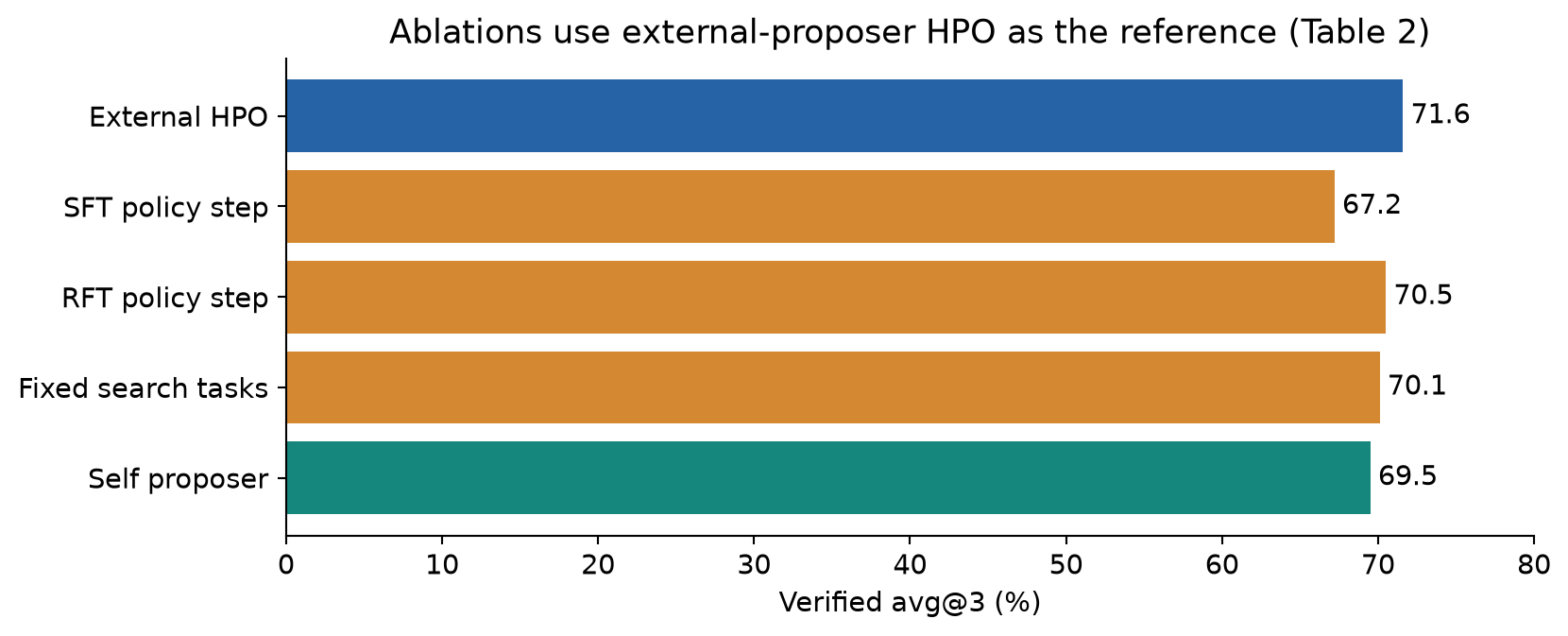
Figure 7. Table 2 means, with the reference explicitly identified. These results are not four independent ablations starting from the 69.5 Self-HPO configuration.

The gap between RL and SFT supports the use of reinforcement learning in this setup. The smaller gap to rejection-sampling fine-tuning suggests that successful on-policy experience itself is valuable, with an additional benefit from the RL objective and sampling procedure. However, comparing final resolve rates alone cannot isolate every contribution of the objective, data distribution, and number of generated trajectories.

The fixed-search-set result supports refreshing the failure targets as the solver changes. Its 1.5-point deficit is consistent with early-policy failures becoming stale. It does not tell us whether “never solved” is the best refresh criterion, because the experiment compares refresh against no refresh rather than against a range of alternative curricula.

Finally, the 2.1-point self-proposer deficit measures the cost of removing the external proposer under the reported conditions. It should not be added to the SFT or fixed-set deficits to forecast a new combination: interventions can interact. A factorial experiment would be needed to estimate such interactions rather than assuming the ablation penalties are additive.

12. pass@k, difficulty buckets, and the meaning of a frontier

The pass@k analysis uses eight attempts per task on Verified. If $c$ of $n=8$ attempts succeed, the usual estimator for success within $k$ draws without replacement is

$$\widehat{\operatorname{pass@}k} =1-\frac{\binom{n-c}{k}}{\binom nk},\qquad n=8. \tag{8}$$

The ratio is the probability of choosing only failed attempts; subtracting it gives the chance of including a success. If fewer than $k$ failures exist, the numerator is zero. The estimator is computed per task and then averaged. At $k=1$, it reduces to $c/n$; at $k=n$, it is one exactly when at least one of the eight attempts succeeds. The paper supplies bootstrap 95% confidence intervals for this analysis. [1, Figure 4]

Self-HPO improves pass@8 from 80.0% to 84.8%, a 4.8-point gain. This is evidence that successful trajectories appear for more tasks in the sampled attempts, not only that an already-existing success becomes more frequent. But the word “frontier” should stay tied to the sampled budget: eight failures under the base do not establish that a task is impossible for that policy.

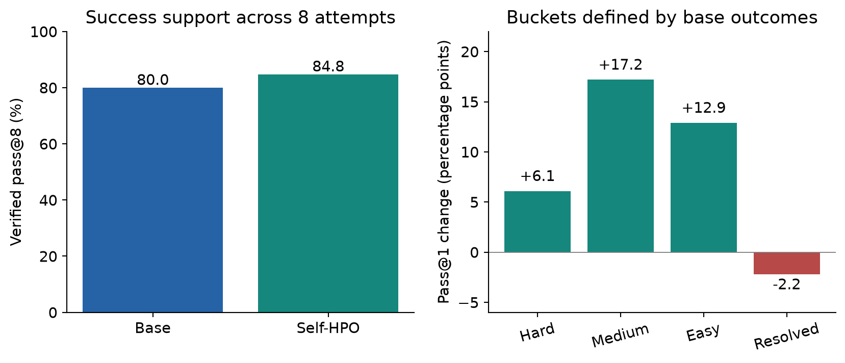
Figure 8. Reported values from Figure 4: pass@8 on the left and pass@1 changes within base-defined task buckets on the right. Only explicitly reported values are plotted; no intermediate pass@k points have been inferred.

The base agent’s observed success frequency defines four buckets: hard tasks have no successes; medium tasks have a frequency above zero and at most one half; easy tasks have a frequency above one half but below one; resolved tasks succeed on all sampled attempts. Self-HPO gains 6.1, 17.2, and 12.9 points in the first three buckets but loses 2.2 points in the last.

That loss is important. Additional controls can interrupt a trajectory that the original system already handles well. The result also cautions against a simplistic narrative in which every harness mechanism is a universally beneficial safeguard. The buckets are selected using the base’s outcomes, so selection effects and regression to the mean can influence comparisons. The observed pattern is useful evidence of heterogeneous effects, not a clean estimate of each task’s true difficulty.

During the final Self-HPO P-step, the fraction of zero-success rollout groups falls to 6.5% averaged over the last ten updates. RLVR remains mostly between 11% and 17% over its last fifty updates. This supports the proposed learning-signal mechanism, but the two summaries use different aggregation windows. They should not be converted into a precise relative reduction without matching the windows and the underlying task exposure.

13. What the harness changes: two examples that must stay separate

Figure 5 and Appendix D describe the harness produced by external-proposer HPO. Its controls include a budget warning before exhaustion, a one-time guard against an empty patch, a one-time hold on the first nonempty submission asking the model to ground API names and signatures in repository tests, and a fallback to the sandbox’s diff when the submitted patch cannot be applied. These mechanisms act on context, behavior, and termination rather than only on the initial instruction.

Each control has a reason and a boundary. A budget warning can prevent a useful working-tree edit from being lost, but an early warning can also encourage premature completion. An empty-patch check can recover a missing artifact, but it needs a clear rule for tasks where no change is appropriate. Asking for API grounding can prevent plausible but nonexistent interfaces, but repeated requests can waste time after the relevant checks have already been done. A fallback diff can recover omitted edits, but it must avoid including unrelated workspace changes.

Those are not a definitive list of the exact mechanisms learned by Self-HPO. Appendix E instead gives a trajectory example from the self-improving configuration, on task sphinx-doc__sphinx-9658. Under $H_0$, the final policy makes edits and passes a reported set of 99 tests, yet returns a summary instead of the required patch. Under $H_2$, another trajectory passes 195 tests and initially tries to submit a source excerpt. A touched-file versus submitted-patch coverage check notices that a file was edited but no file is present in the submitted patch. The harness holds completion once, giving the policy a chance to generate and submit a proper diff.

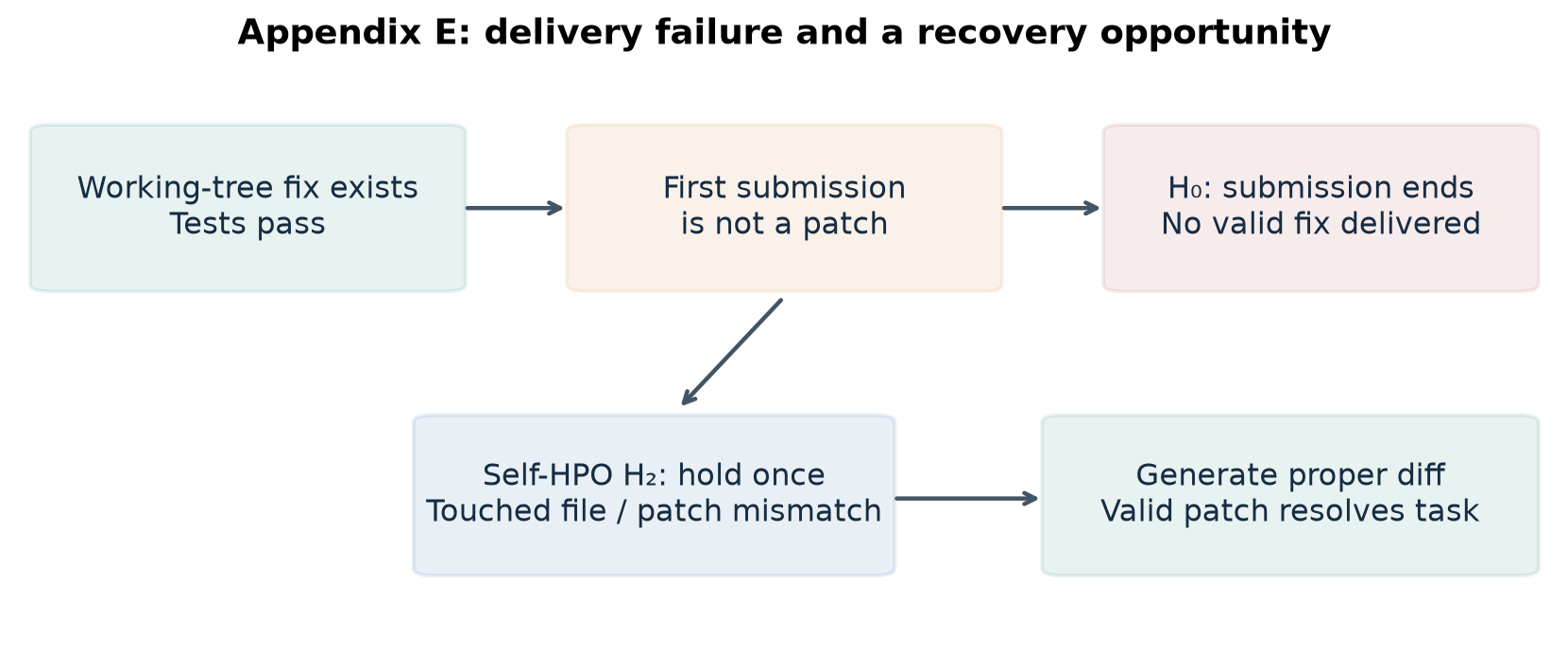
Figure 9. Conceptual summary of Appendix E’s Self-HPO example. The two trajectories differ, so the branches illustrate a delivery failure and a recovery path; they are not a paired counterfactual with an identical prefix.

The appendix also documents a faulty reminder. A PR-intent check extracts keywords from the issue text that are not actually central to the repair, producing a false-positive warning. This is valuable negative evidence. A general rule inferred from failure traces can improve one part of the interaction while adding a misleading intervention elsewhere.

The example explains how a harness can turn existing repair work into a delivered success. It does not quantify how much of the overall 8.5-point gain comes from this mechanism, and it does not prove that holding the submission alone caused the difference between the two trajectories. They take different actions, run different numbers of tests, and have different histories. A controlled intervention at an identical pre-submission state would be needed for that stronger causal claim.

14. Cost accounting: accepted trajectories are only the visible tip

The reported training schedule uses $2\times50\times128=12{,}800$ accepted trajectories across its policy updates. This arithmetic describes training inputs, not total environment episodes. Eight trajectories are sampled before four are selected, and additional sampling is needed when a task cannot supply a balanced group. Episode length also varies, so even the generated trajectory count would not be a complete token-cost estimate.

For the first harness search, six candidates evaluated on 300 tasks require 1,800 candidate-task rollouts, plus 300 rollouts for the incoming harness, before counting proposal generation or infrastructure retries. The later search set has a data-dependent size. It would be misleading to multiply 300 by every later search round without establishing that the set remains that large.

A useful total-cost decomposition is

$$C_{\mathrm{total}}=C_{\mathrm{proposals}}+ C_{\mathrm{search\ rollouts}}+C_{\mathrm{RL\ rollouts}}+ C_{\mathrm{optimization}}+C_{\mathrm{evaluation}}. \tag{9}$$

This is a bookkeeping proposal for evaluating the method, not a cost model fitted by the authors. A comparison should record wall time, generated assistant and tool-context tokens, verifier time, rollout acceptance rate, and the quality of the resulting agent. Faster optimization steps can coexist with a larger rollout bill, while a more reliable final agent can repay an expensive training phase over many deployments.

Search itself has an opportunity cost. If a fixed budget buys either more policy training or another harness round, the correct decision depends on which failure modes remain. Delivery failures suggest harness work; repeated semantically incorrect patches may require better policy learning or data. The paper demonstrates one successful allocation, but does not map the full frontier between search effort and training effort.

15. Limitations supported by the evidence

First, the experiments use one base model family and two alternating rounds. The results do not establish that weaker initial models can propose useful controls, that larger models benefit by the same amount, or that long chains of updates remain stable. A process that works for two rounds can later accumulate contradictory checks or become trapped by its own training interface.

Second, task distribution and verification remain central. The training tasks come from Python software repair, while transfer is tested on additional repair benchmarks. That is meaningful transfer, but it is still within software engineering. Scientific exploration, open-ended planning, and tasks with subjective outcomes have different feedback conditions. The method’s binary verifier is an asset that those settings may not share.

Third, the search score is noisy and adaptive. Repeatedly selecting the best of a small candidate sequence on the same tasks can exploit evaluation noise or particular task features. The final benchmarks provide an external check, but the paper does not establish a general statistical guarantee for every search-step acceptance decision.

Fourth, the evidence does not fully decompose success. A valid patch is required for the benchmark, so improved delivery is a legitimate gain. Yet it is analytically different from expanding the set of semantic fixes the model can discover. The appendix proves the relevance of delivery failure as a phenomenon; it does not assign an aggregate percentage of gains to delivery versus reasoning.

Fifth, the cross matrix reveals some interface dependence, and the difficulty analysis reveals regressions among initially reliable tasks. These are not contradictions of the main result. They describe its scope: a better average pair can coexist with a less portable policy and with losses on a subset of tasks.

16. Critical analysis: what would make the causal story stronger?

My central reading is that the paper identifies a useful feedback loop but only partially measures its internal causes. A better harness can improve the distribution of learning experiences; a better policy can then propose or exploit a better harness. The reported outcomes and ablations support this account. To establish how much each channel contributes, the next experiments should separate behavioral opportunity, policy learning, and artifact delivery.

One useful intervention would save pre-submission states and replay them under alternative termination rules with the same policy and controlled sampling. Measure three quantities separately: whether a correct working-tree edit exists, whether a valid patch is delivered, and whether that patch passes the verifier. This would quantify delivery yield without attributing all of it to deeper repair ability. It would also reveal cases in which a safety-like reminder destroys an already-correct completion.

A second experiment would train under several harnesses and evaluate on held-out interfaces. The current cross matrix is already a good start, but its checkpoints all arise along one coupled trajectory. A broader matrix could distinguish portable repair knowledge from adaptation to a particular sequence of feedback messages. The relevant target is not invariance to every arbitrary interface; it is robustness to reasonable changes in tool formatting, submission protocol, and failure feedback.

Third, the 1.6-point interaction contrast deserves task-level uncertainty. A paired bootstrap over tasks could preserve the relationship between outcomes from the four compared configurations, while multiple independent search-and-training seeds would capture procedure-level variability. Reporting only marginal standard deviations cannot show whether the interaction is stable. This matters because the final joint advantage can be real even if the precise superadditive contrast is uncertain.

Fourth, the never-solved curriculum should be compared with alternatives that control for exposure. A task with no success in two attempts should not automatically be treated as equivalent evidence to one with no success in twenty. Stratifying by attempts, estimated success probability, and failure type would test whether the benefit comes from refreshing tasks at all or from the specific zero-success rule. A small stable regression set would also protect tasks already handled well.

Fifth, mechanism addition should eventually be paired with deletion and compression. The proposal constraint of adding one control aids local interpretability, but it can make the harness an archive of past weaknesses. Some controls may become obsolete once RL internalizes the desired behavior. An ablation that periodically removes redundant controls would test whether the loop learns durable capabilities or merely accumulates scaffolding.

Finally, the resource comparison should count every generated rollout and separate external-model supervision from self-proposal. Self-HPO’s lack of a stronger proposer is a meaningful design property. It is not equivalent to having no external knowledge: the initial pretrained model, curated repair tasks, reference fixes available during diagnosis, and executable tests all contribute information. Clear accounting strengthens the result more than a broad claim of autonomous improvement would.

17. Conclusion: optimize the pair, then test what survives separation

Self-HPO provides concrete evidence that harness search and policy RL can reinforce one another. Its final self-improving agent beats both harness-only and policy-only baselines across three repair benchmarks, and the crossed-checkpoint table shows that each evolved component retains some value on its own. The pass@8 result further indicates that the gain is not limited to increasing success frequency on an unchanged set of sampled tasks.

The most useful lesson is methodological. An agent’s learning environment includes the interface that shapes observations, recovery opportunities, and completion. Improving that interface can change which trajectories supply useful rewards. But a strong final pair should still be tested by separating its components, examining regressions, and measuring the cost of producing its training data.

The paper is persuasive as a two-round demonstration of coupled optimization. Its open questions concern portability, causal attribution, long-run control accumulation, and cost. Those questions make HASE’s joint action-space approach and HarnessBandit’s multi-harness scheduling natural next readings; they address adjacent ways of coupling interface behavior with policy learning, rather than merely repeating the same search procedure.

References and figure provenance

1. Zhepei Wei, Wenlin Yao, Baolin Peng, Danqing Wang, Qianhui Wu, Hao Cheng, Yu Meng, and Jianfeng Gao. Self-Evolving Coding Agents via Harness-Policy Optimization, v1, 2026-10-16. The main text and Appendices A–E are the technical source for this review. Equation (1), the optimization procedure, the training settings, Tables 1–3, Figure 4, and Appendix E provide the specific evidence discussed above.
2. Haochen Luo et al. Harness-Aware Self-Evolving: Co-Evolving Model Weights, Harness, and Task Solutions, 2026-07-04. Added as a future reading on joint solution and harness actions; it is not an additional baseline measured in this review.
3. Hongliang Wei et al. HarnessBandit: Joint Learnability-Transferability Scheduling for Multi-Harness Agentic Reinforcement Learning, 2026-09-12. Added as a future reading on training across multiple harnesses.

All nine figures were prepared for this review. Figures 1–2 and 9 are explanatory reconstructions, Figures 3–4 are explicitly labeled analytical illustrations, and Figures 5–8 redraw reported values from the source. No new empirical results, replication claims, or interpolated benchmark measurements are presented.