RRSI: When Should a Self-Evolving Agent Keep Its Changes?

Review date: October 26, 2026. Paper: RRSI: Regularized Recursive Self-Improvement of Agent Harnesses. Authors: Peng Xia, Rujun Han, Zifeng Wang, Yanfei Chen, Yufan Zhuang, Yoonho Lee, Chengsong Huang, Han Yu, Zhongying CuiZhu, Yifei Ming, Huaxiu Yao, Burak Gokturk, Tomas Pfister, and Chen-Yu Lee. Version: arXiv:2609.24972v3, revised October 4, 2026. Paper · Authors’ project · Code resource.

This review covers the 27-page paper and Appendices A–F. Experimental numbers are the authors’ reports; calculations, illustrative examples, and proposed follow-up experiments are identified as such. The arXiv version date is used above; the PDF’s internal cover date is October 6. No new agent benchmark experiments are reported here.

1. Improving the score is easier than improving the agent

Imagine an agent that must prepare a spreadsheet, a memo, and a supporting calculation. A failed run may reveal a missing source value, an unchecked formula, or an output filename the agent never created. Adding a small check before completion could help many future tasks. Adding a long checklist that repeats the current benchmark’s rubric could also raise the measured score. Both changes can look successful on the examples that suggested them. Only one may remain useful when the task changes.

RRSI studies this distinction at the level of the harness: the prompts, tools, memory, context management, and control flow around a frozen language model. Recursive self-improvement here means repeatedly using agent outcomes to modify this surrounding system. It does not mean that the model retrains its weights, proves its own correctness, or acquires an unlimited capacity to improve. The optimization variable is an executable agent design evaluated under a finite search budget.

The central concern is adaptive overfitting. A proposer sees failures from the same task collection, invents changes, receives scores on that collection, and repeats. Even if it never sees an answer key, its decisions increasingly depend on the peculiarities of the measured tasks. The search can learn the document genre, the preferred presentation style, or a lucky pattern in stochastic evaluations. It can also spend more inference tokens and misdescribe that expense as a better mechanism.

The authors’ response is to regulate the transition between harnesses. They leave the kinds of components editable, but limit how many independent changes may travel together; preserve evidence from failed proposals; direct stalled search toward less explored components; screen candidate changes; and impose score and cost conditions before a candidate can survive. The resulting method is a collection of operational constraints, not a new differentiable training objective.

The most informative result is a reversal of rankings. On Harvey LAB’s evolve split, Meta-Harness rises from 89.4 to 93.0 while RRSI reaches only 90.5. On the mean of three unseen workspace benchmarks, the corresponding scores are approximately 40.6 and 43.6, from a base near 39.7. A method can therefore be less successful at exploiting its immediate feedback yet more useful elsewhere. That is the empirical claim worth testing; “self-improvement” alone is too broad a label to establish it.

2. Prerequisites: what the measurements actually represent

Write an agent as $A=(\pi,H)$, where $\pi$ is the fixed policy and $H$ is the harness. For a task $x$, the agent samples an interaction trajectory $\tau$ and receives reward $r(x,\tau)\in[0,1]$. Its cost $c(\tau)$ counts policy tokens. The paper’s population quantities are

$$S(H;D)=\mathbb{E}_{x\sim D}\mathbb{E}_{\tau\sim A(\cdot\mid x)}r(x,\tau),\qquad C(H;D)=\mathbb{E}_{x\sim D}\mathbb{E}_{\tau\sim A(\cdot\mid x)}c(\tau).$$

There are two levels of averaging: across tasks and across stochastic trajectories for the same task. With $k$ trials per task, an ordinary equally weighted empirical estimate would be

$$\widehat S(H)=\frac{1}{k|D|}\sum_{x\in D}\sum_{j=1}^{k}r(x,\tau_x^{(j)}),\qquad \widehat C(H)=\frac{1}{k|D|}\sum_{x\in D}\sum_{j=1}^{k}c(\tau_x^{(j)}).$$

First compute the outcome of each rollout, then average the $k$ outcomes of a task, then aggregate tasks. This explains why an extra solved rollout is not automatically an extra solved task. In coding, 89 tasks and two trials produce 178 trial outcomes; one additional pass changes the reported fraction by $1/178$, or about 0.562 percentage points. It also explains why trials from the same task should not be treated as independent task samples in a confidence interval.

Actual benchmarks do not all use the simple equal-task average. Appendix B says Harvey LAB aggregates criterion verdicts: tasks with longer rubrics carry greater weight. JobBench uses its weighted rubric, GDPval compares deliverables with human reference work, and Frontier-Eng uses medal credit. The notation gives a useful abstraction, but comparisons must retain these operational definitions. A 4-point increase in one benchmark is not a common unit of human utility across all domains.

A second prerequisite is the distinction between a fixed test and an adaptive test. Suppose a fixed candidate has empirical error $\epsilon(H)=\widehat S(H)-S(H)$. A score-maximizing selector chooses an index $J$ using those same errors. The selected estimate obeys

$$\widehat S(H_J)=S(H_J)+\epsilon(H_J),\qquad J=\arg\max_{1\leq j\leq m}\widehat S(H_j).$$

Even if each fixed candidate’s error is centered, the selected error need not be. As an explanatory model, if all candidates have equal true performance and independent Gaussian noise of standard deviation $\sigma$, the maximum noise grows roughly as $\sigma\sqrt{2\log m}$ for large $m$. This is a pedagogical approximation, not an RRSI theorem: real candidates are correlated and later proposals depend on earlier results. Its purpose is to show why more search can produce more optimism without producing more transferable capability.

Finally, distinguish search uncertainty from evaluation uncertainty. Re-running an evaluation of one fixed harness tests rollout or task variation. Re-running the entire evolutionary process tests whether different proposals lead to comparable final agents. RRSI includes evidence about both, but those experiments answer different questions and have different sample sizes.

3. The architecture of a regularized transition

The paper separates a proposal stage from a selection stage. The proposer receives the incumbent harness, current failure feedback, a history of measured edits, a changing edit budget, exploration directives, and deletion targets. The selector evaluates only candidates that survive a preliminary screen. It then combines a global score floor, a branch-specific cost rule, and any domain guards.

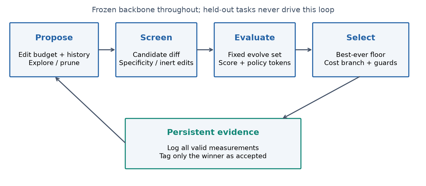
Figure 1. Original explanatory diagram based on Section 3 and Appendix D. All valid measurements contribute evidence; only the selected winner becomes the next accepted harness. Held-out feedback is outside this loop.

The distinction between open edit space and constrained proposal matters. A component can remain legally editable while rarely receiving proposal capacity. Limiting an update to two atomic changes does not forbid adding a memory component over the whole run. It does, however, discourage a proposal that simultaneously rewrites memory, tool routing, stopping, and the system prompt. That makes the effect of a successful proposal less ambiguous.

The paper calls the update budget $L_0$-like, structural pruning $L_1$-like, and resource control $L_2$-like. These are functional analogies. There is no common continuous parameter vector whose norm is minimized. In particular, a token-growth inequality is not ridge regression, and removing an unused tool is not the solution of a lasso objective. The analogy is useful only if it helps identify three distinct interventions: sparse changes, deletion of structure, and restraint on aggregate resource use.

A conventional scalar objective, such as score minus a token penalty, would let enough improvement compensate for any other defect. RRSI uses several non-compensatory gates. A very cheap candidate cannot buy its way below the global score floor. A high-scoring benchmark-specific change should be rejected before its score enters selection. This creates a different decision geometry from a single weighted sum, although it still leaves room for subjective or incompletely specified guards.

4. Proposal regularization: capacity, memory, and exploration

4.1 Why the budget is attached to an update

Let an update select atomic edits with binary vector $z_t$ from a newly drafted pool. The cardinality constraint is $\|z_t\|_0\leq b_t$. The pool can change at every round, so the vector has no fixed interpretation across the run. The published schedule is

$$b_t=\left\lceil b_{\min}+(b_{\max}-b_{\min})\frac{1+\cos(\pi t/T)}{2}\right\rceil.$$

At $t=0$, the cosine is one, so the expression is $b_{\max}$. At $t=T/2$, the continuous budget is the midpoint of the two bounds. At $t=T$, it reaches $b_{\min}$. The derivative of the continuous envelope is non-positive over that interval, which gives a smooth decrease before integer rounding. Early coordinated changes remain possible; late changes are intended to become easier to attribute.

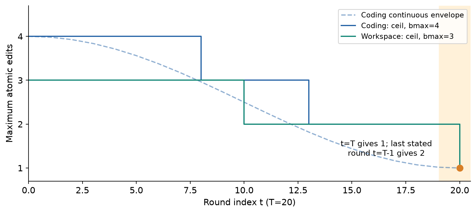
Figure 2. Calculation from Equation 4 and Table 5, not a measured evolution trace. The endpoint at $t=T$ is shown explicitly because Appendix D states rounds $0$ through $T-1$.

There is a small but consequential specification issue. With ceiling rounding, $b_{\min}=1$, and the stated loop stopping at $T-1$, the last evaluated budget is two rather than one for the listed horizons and maxima. For coding, $T=20$ and $b_{\max}=4$ give a last continuous value just above one. The prose’s promise of a final single-edit round therefore needs an indexing or rounding clarification. I retain the printed formula rather than silently substituting a schedule that fulfills the prose.

More generally, a sparse edit is not necessarily a simple behavioral change. One added instruction can alter many decisions, while a coordinated two-file repair can be one mechanism. The meaningful unit is an independently attributable intervention, not a line count. The method relies on assigning these units consistently; this is a modeling choice whose reliability deserves evaluation.

4.2 History provides evidence, not causal attribution

The edit history records the round, component, hypothesis, change description, score difference, relative cost difference, and acceptance indicator. Every measured edit in a bundled candidate inherits the same candidate-level outcome. Rejected but evaluated candidates remain in this history. An admissible candidate that loses to a higher-scoring candidate is also marked unaccepted; rejection does not always mean the mechanism was harmful.

This prevents the proposer from treating every round as a fresh brainstorming session. A previous failed retry policy remains evidence against trying essentially the same policy again. But the history is observational. If a candidate combines an improved completion check with a harmful memory expansion and obtains a positive net change, both components inherit positive credit. Annealing reduces that ambiguity but does not remove interactions or measurement noise.

For a component $\ell$, Appendix D summarizes recent evidence by

$$g_t(\ell)=\max\{\Delta S_i:\ell_i=\ell,\ t-t_i\leq n_{\mathrm{prune}}\},\qquad B_t=\{\ell\in\mathcal T_t:g_t(\ell)\leq0\}.$$

Here $\mathcal T_t$ contains components previously exercised by a valid measured edit; an empty recent set has maximum $-\infty$. This convention means that a component with only old evidence can become a pruning target. The maximum is also forgiving: one small positive recent observation can prevent a target from being marked unproductive. Neither property is a statistical demonstration that the component is useful or useless.

Pruning targets are instructions for subsequent proposals, not immediate deletions bypassing evaluation. That is an important safeguard for components whose value appears only in combination with others. A proposed deletion still has to survive the selector. An alternative would measure each component’s marginal contribution with controlled ablations, but that would consume substantially more evaluation budget.

4.3 Stalls change where the search looks

The stall indicator checks whether progress over a window exceeds the noise tolerance: $\sigma_t=\mathbf1[\widehat S_t-\widehat S_{t-w}\leq\delta]$. If not, an exploration slot is reserved for components that have never been measured. All settings use $w=3$ and reserve one of two candidate slots, so exploration can occupy half a round. This is not a tiny continuous perturbation of the search distribution.

“Never measured” is different from “never accepted.” The exploration set is based on measured history, whereas the within-band novelty bonus later uses accepted history and only four structural categories. Once every category has been measured, the untried set can become empty; the paper does not thereby establish broad behavioral diversity. A proposer can exhaust the component labels while remaining trapped in a narrow family of mechanisms.

Algorithm 1. A proposal round, reconstructed from Appendix D

Input: incumbent H, measured history L, round t, horizon T
1. Analyze current evolve-task failures and summarize feedback.
2. Compute the published cosine edit budget b(t).
3. Test whether progress over the stall window exceeds delta.
4. Find component types with no valid measured edits so far.
5. If stalled, reserve the configured exploration candidate slot.
6. Find previously exercised components with no recent positive gain.
7. Propose candidates using feedback, history, budget and targets.
8. Tag each atomic edit with its component and hypothesis.
9. Screen actual candidate changes for specificity and inert additions.
10. Return the screened candidates for full evolve-set evaluation.

This pseudocode expresses the paper’s procedure, not a new experiment. Initial-window handling and the exact domain guards must be specified before treating it as a complete operational protocol. The gain from this structure is disciplined use of evidence; it should not be mistaken for proof that the proposer’s diagnoses are correct.

5. Selection: what a candidate must earn

5.1 A critic is a filter, not a transfer test

Before full evaluation, a critic examines the actual candidate changes for task names, entities, answers, task-specific constants, and inert machinery. The timing prevents an explicitly leaking candidate from first receiving a spectacular score and influencing later reasoning. The critic is meant to inspect the changed harness, rather than reject a proposal merely because its explanatory rationale names a task.

Appendix F reports 38 screened coding candidates and one outright rejection, related to a mismatch between the declared component and the actual change. This is evidence about what happened in that run, not a calibrated false-negative rate. A filter can reject literal memorization while missing a generic-looking rule that happens to fit the search distribution. Conversely, a benchmark-named tool can implement a reusable action. Generality is ultimately a behavioral property, not a vocabulary property.

The same model family supplies policy, proposer, analyst, and critic in the main experiments. That simplifies the comparison but permits correlated blind spots. A plausible diagnosis may look equally plausible to the critic. A cross-family critic or deliberately planted specificity cases would help evaluate this component separately. Neither is necessary to appreciate the overall transfer results, but both matter before attributing those results specifically to leakage detection.

5.2 The floor is anchored to the best accepted score

Let $S^\star$ be the non-decreasing best score along the accepted path. The candidate must satisfy

$$\widehat S(H')\geq S^\star-\delta,\qquad S^\star_{t+1}=\max\{S^\star_t,\widehat S(H_{t+1})\}.$$

The main text describes a best score “observed so far,” but Algorithm 2 updates it from the next accepted harness. I use that algorithmic definition: a high-scoring candidate rejected for cost does not automatically move the acceptance floor. This distinction affects later admissibility and should not be erased in a simplified explanation.

To see why the anchor matters, consider a hypothetical incumbent at 90.0 and tolerance 0.4 percentage point. A rule comparing only with the current incumbent could accept 89.7, then 89.4, then 89.1: every individual decline is within tolerance, but the total loss is not. An unchanged best-ever anchor at 90.0 keeps the lower bound at 89.6. The second of those replacements fails regardless of its token savings.

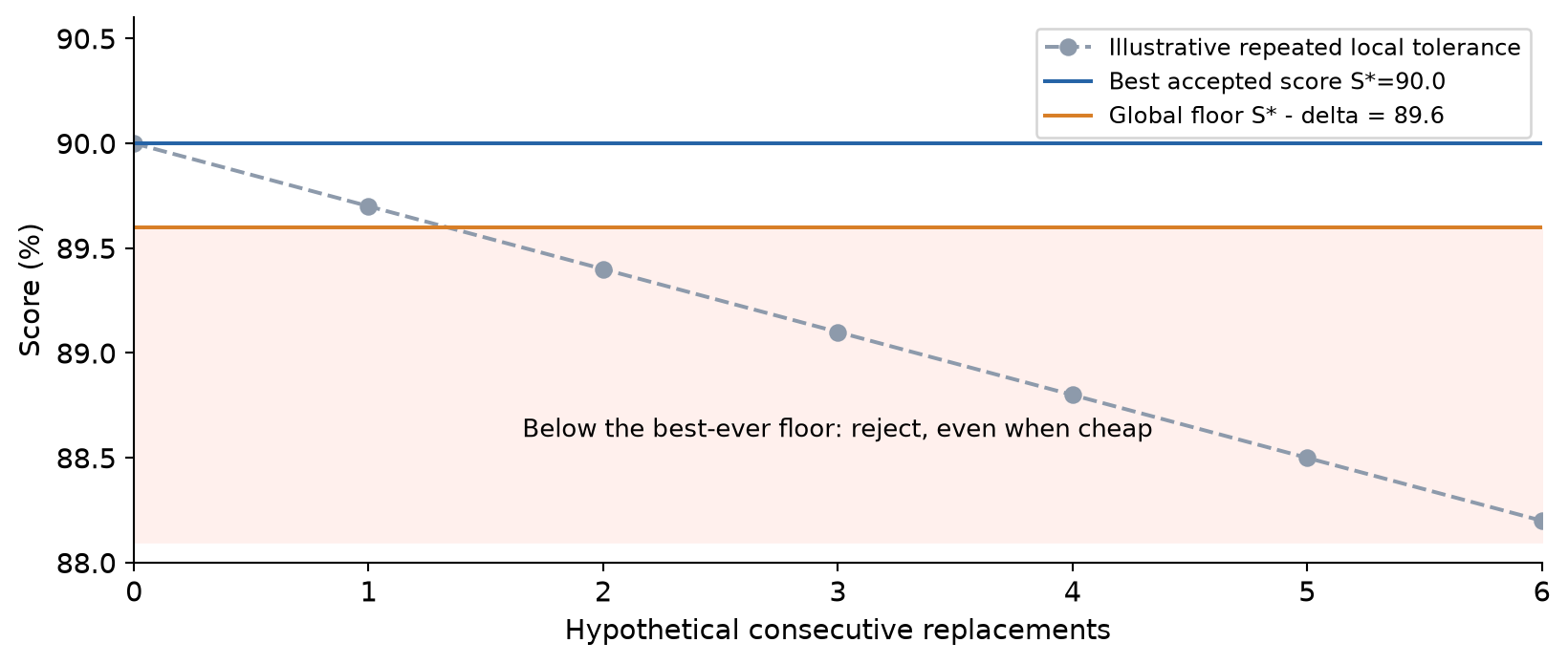
Figure 3. Hypothetical numerical example illustrating the floor. It is not a trajectory reported by the authors.

This is protection against downward drift, not a proof of statistical significance. The empirical band is calibrated from repeated unchanged-harness evaluations, rather than derived as a simultaneous confidence bound for an adaptive search. A lucky accepted high score can also make the floor too demanding. Candidate-dependent variance, task correlations, and repeated comparisons remain relevant even with a non-decreasing reference.

5.3 Large gains must justify their extra tokens

Relative to the current harness, define

$$\Delta S=\widehat S(H')-\widehat S(H_t),\qquad \Delta C=\frac{\widehat C(H')-\widehat C(H_t)}{\widehat C(H_t)}.$$

The score difference is in fraction units, whereas the cost difference is a relative increase. If $\Delta S>\delta$, the cost gate requires $\Delta C\leq\beta_0+\beta_1\Delta S$. A positive intercept permits some overhead, and the slope specifies how much extra cost a measured improvement can buy. For coding, $\beta_0=0.10$ and $\beta_1=44.5$.

Converting the coding units step by step makes the large-looking slope intelligible. Seven extra passes out of 178 outcomes give $\Delta S=7/178\approx0.03933$. Multiplying by 44.5 yields 1.75; adding the 0.10 intercept gives a maximum relative increase of 1.85, or 185%. Appendix E describes a candidate with 130% growth that therefore fits this allowance. This gate can tolerate a final cost of 2.85 times the incumbent; “regularized” does not mean “small overhead.”

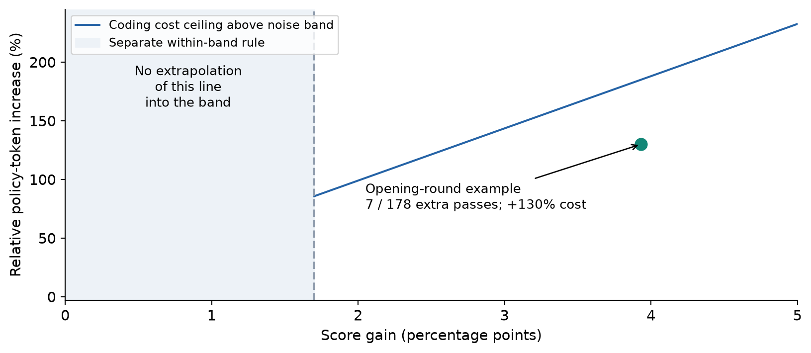
Figure 4. Calculated threshold from Table 5, with the opening-round example in Appendix E.1. The shaded region uses a different rule; extending the line into that region would misstate the algorithm.

The distinction between points and fractions is critical. Inserting 3.93 instead of 0.0393 multiplies the score-dependent allowance by 100. Similarly, 130% relative growth is $\Delta C=1.30$, not 130. These conversions are mundane, but they determine whether the acceptance rule is restrictive at all.

The paper calibrates these allowances against benchmark units and opening-round candidate behavior, then keeps them fixed for transfer. This is more defensible than tuning against OOD scores, but it still reflects design decisions informed by the evolution environment. A different score scale or deployment budget would require a new calibration; the coefficients are not universal constants.

5.4 Small gains use a separate shaped condition

When the candidate clears the global floor but $\Delta S\leq\delta$, the rule becomes

$$w_s\Delta S-w_c\Delta C+w_n\nu_t(H')>0, \qquad \nu_t(H')=\sum_{\ell\in\mathcal K_{\mathrm{str}}} \mathbf1[\ell\in\operatorname{comp}(H')\ \land\ N_t(\ell)=0].$$

The set $\mathcal K_{\mathrm{str}}$ contains client tools, skills, memory, and subagents. $N_t(\ell)$ counts previously accepted edit records for a component type. The novelty bonus therefore rewards touching an as-yet-unaccepted structural category; it is not a semantic distance from earlier candidates. Prompt, control-flow, configuration, output-plumbing, and context-management edits receive no such bonus.

For coding, the paper states $w_s=0$. A within-band score increase cannot by itself qualify a coding candidate. Cost reduction contributes positively because $\Delta C<0$ makes $-w_c\Delta C>0$; structural novelty can also contribute. For workspace and engineering, $w_s$ is positive, so small score changes do retain weight. The informal slogan that small gains receive no credit is thus not equally true across domains.

Appendix D says the three weights are reported in Table 5, but the displayed table does not list them. This leaves the exact within-band decision boundary incomplete in the paper. We can explain its direction and the coding special case, but cannot infer the missing numerical settings. Nor should we use the large-gain cost line to fill that gap: the text explicitly says Equation 7 is not used in this branch.

Algorithm 2. Select a successor using the published gates

Input: screened candidates, incumbent (H, S, C), best score Sstar
1. Evaluate each candidate on the fixed evolve set with k trials.
2. Compute deltaS relative to S and relative token change deltaC.
3. Count newly accepted-type structural novelty for the candidate.
4. If deltaS > delta:
       cost_ok = deltaC <= beta0 + beta1 * deltaS
5. Otherwise:
       cost_ok = ws * deltaS - wc * deltaC + wn * novelty > 0
6. Require score >= Sstar - delta and the relevant domain guards.
7. Keep candidates passing every required gate, including cost_ok.
8. Select the highest-scoring admissible candidate; if none, keep H.
9. Update Sstar using the score of the resulting accepted harness.
10. Record every valid measurement; mark only the new winner accepted.

This selector can move to a slightly lower-scoring candidate if it remains within the global band and qualifies through cost or novelty. It is therefore not identical to greedy monotone score improvement. The shaping rule determines admissibility, but final ranking among admissible candidates is by empirical score. A large novelty bonus does not itself become the final ranking objective.

6. What the experiments compare

The main experiments use a frozen Claude Opus 4.8 policy, with the same model for proposal, analysis, and criticism. Coding starts from Terminus-2. Workspace and engineering use a ReAct-style loop with a tool gateway, dynamic tool selection, and context management. Baselines share the initial harness, frozen policy, evolve tasks, and candidate budget. This isolates the search strategy more closely than comparing unrelated off-the-shelf agents, although equal candidate count does not imply equal total optimization compute.

There are three separate evolution environments and five OOD benchmarks, plus one ID held-out split. This is eight benchmarks and nine reported splits, not nine independent domains. Coding evolves on all 89 Terminal-Bench 2.1 tasks and transfers to SWE-bench Verified. Workspace evolves on 120 Harvey LAB tasks, retains 40 Harvey tasks for ID testing, and transfers to JobBench, GDPval, and APEX-Agents. Engineering evolves on 61 license-free EngDesign tasks and transfers to Frontier-Eng.

Setting	Rounds	Trials per task	Noise tolerance	Initial edit cap	Pruning window
Coding	20	2	0.017	4	4
Workspace	20	2	0.004	3	4
Engineering	40	4	0.020	4	5

Table 1 of this review transcribes part of the paper’s Table 5. The tolerance is in fraction units: 0.017 is 1.7 percentage points. All settings list a minimum edit cap of one, a three-round stall window, and one exploratory candidate out of two. The endpoint caveat in Section 4 still applies.

The scoring protocols deserve as much attention as the model names. Terminal tasks use hidden tests and fresh containers between arms. SWE-bench requires both fail-to-pass repair and preservation of pass-to-pass behavior. Harvey grades individual rubric criteria, with missing deliverables failing their associated criteria. APEX reports over all 480 tasks, counting missing rollouts as failures rather than dropping them. These choices prevent some superficially successful but invalid comparisons.

Engineering offers a useful complementary check because the evaluators are deterministic simulators or testbenches. That removes judge sampling from grading, but it does not make the agent deterministic or eliminate overfitting to the task collection. For Frontier-Eng, the EngDesign-overlap domain is excluded, and unbuildable environments receive no credit in both arms; the paper says 38 of 47 tasks contribute credit. The reported medal score should not be relabeled a solve rate.

GDPval’s description also needs clarification. Appendix B.5 names 185 tasks and judging in both presentation orders, but then states 204 comparisons per judge per harness. Those counts do not reconcile under the obvious full-panel interpretation. I use the published win-rate result as reported and do not derive a sample size or standard error from that unexplained 204. Transparent handling of such ambiguity is better than silently choosing a denominator.

7. Main results: transfer changes the ranking

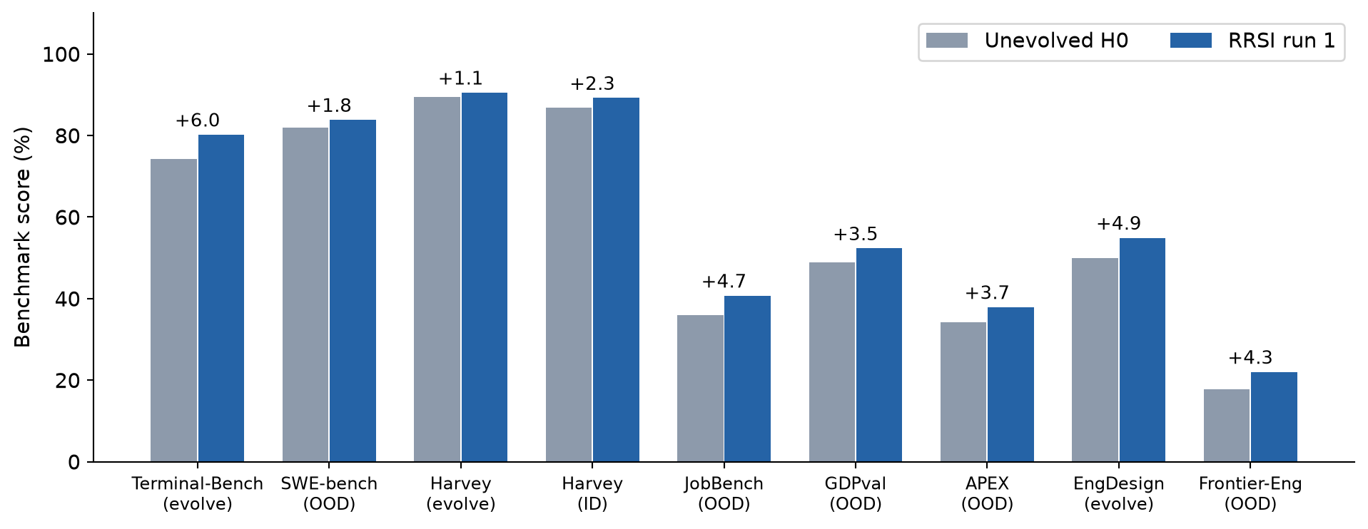
Figure 5. Redrawn from Figure 3 and Table 7. All bars retain their benchmark-specific score definitions. Labels are point gains; the zero-based axis avoids magnifying small improvements.

RRSI’s first main run improves all six splits not used for evolution. SWE-bench rises from 82.0 to 83.8, Harvey ID from 86.9 to 89.2, JobBench from 36.0 to 40.7, GDPval from 48.8 to 52.3, APEX from 34.2 to 37.9, and Frontier-Eng from 17.7 to 22.0. The evolve gains are 6.0 points in coding, 1.1 in workspace, and 4.9 in engineering.

The strongest direct baseline comparison is the workspace table. Meta-Harness, AHE, TTHE, and HarnessX all increase Harvey’s evolve score more than RRSI does. Their OOD outcomes vary sharply. AHE improves JobBench while worsening GDPval and APEX; TTHE worsens all three. This is why a single evolve score is a poor decision criterion and why even one OOD average should be accompanied by its component scores.

Method	Harvey evolve	Harvey ID	JobBench	GDPval	APEX
Initial harness	89.4	86.9	36.0	48.8	34.2
Meta-Harness	93.0	89.2	37.1	49.1	35.7
AHE	90.7	88.7	37.2	47.2	33.1
TTHE	91.1	88.5	35.2	47.0	31.7
HarnessX	91.8	89.1	36.3	48.5	34.3
RRSI	90.5	89.2	40.7	52.3	37.9

Table 2 reproduces the paper’s Table 1 numerical values. Harvey ID is a tie between RRSI and Meta-Harness at the displayed precision, so “strictly better on every held-out dataset” overstates the table. The distinguishing evidence is the OOD separation.

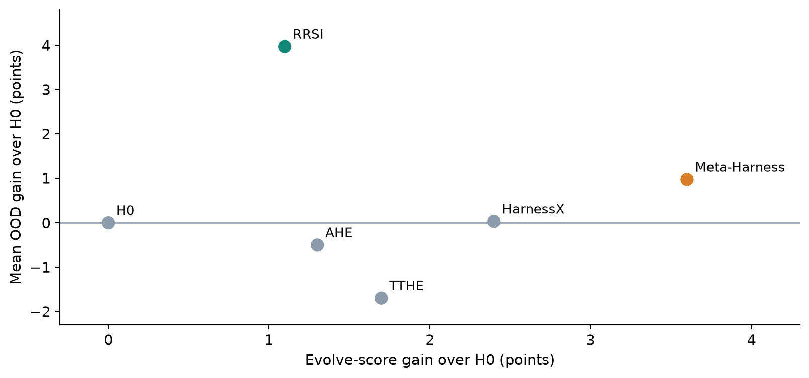
Figure 6. Computed from the displayed Table 1 values. The vertical axis is the unweighted mean gain over the three workspace OOD benchmarks; it is not a pooled success rate over their tasks.

The RRSI OOD mean computed from the rounded entries is $(40.7+52.3+37.9)/3=43.633\ldots$, compared with $39.666\ldots$ for the base. That is about 3.97 points, or 10.0% relative improvement. For Meta-Harness, the same calculation gives 40.633, roughly 0.97 point above the base. The paper’s summary uses rounded 43.6, 39.7, and 40.6, so differences computed only from those summaries may differ by a tenth.

Two headline numbers should not replace the detailed results. The abstract says OOD gains reach 4.3 points, while JobBench in Table 1 and Figure 3 gains 4.7. The engineering gain is indeed 4.3. Likewise, the abstract’s “30% fewer tokens” is not the exact reduction from the unregularized row in Table 2. These discrepancies do not reverse the comparison, but they make table-level attribution necessary.

8. Ablations and the price of a better harness

Table 2 of the paper removes groups of mechanisms, not one mechanism at a time. Without proposal regularizers, workspace OOD average falls from 43.6 to 41.9; without acceptance regularizers it falls to 41.0. Removing both yields 40.3, despite an evolve score of 92.8. The direction is consistent with the method’s motivation: looser search fits the immediate environment better and transfers worse.

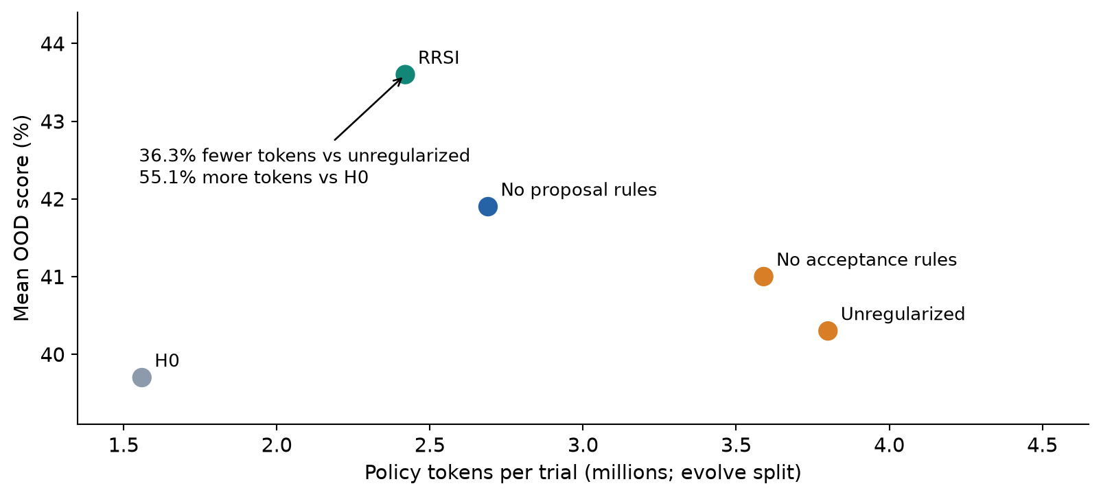
Figure 7. Paper Table 2. Horizontal values measure final-harness execution on the evolve split, not the total compute consumed by proposal, criticism, analysis, or all candidate evaluations.

The cost calculation needs both comparators. RRSI consumes 2.42 million policy tokens per trial, versus 3.80 million for unregularized evolution and 1.56 million for the unevolved harness. Therefore

$$1-\frac{2.42}{3.80}=36.3\%\quad\text{less than unregularized evolution}, \qquad \frac{2.42}{1.56}-1=55.1\%\quad\text{more than the initial harness}.$$

Both statements are true. RRSI restrains the cost of evolution; it does not make the agent cheaper than its starting point. The final harness still buys some capability with additional inference. A full deployment decision would need latency, tool cost, context size, failure recovery, and the amortized cost of searching for the harness. Policy tokens are an informative proxy but not a complete resource account.

The ablations do not establish that every subcomponent is necessary. The acceptance group combines screening, stability, and resource-related decisions; removing it changes several incentives simultaneously. Nor do the two group ablations identify an additive decomposition of benefit. A better proposal can change which candidates a selector ever sees, making their interaction central to the outcome.

The qualitative cases in Appendix F help interpret the numbers. Coding round 0-A adds bounded pre-completion verification and non-blocking polling guidance and is accepted with a 3.93-point gain. A similar round 0-B change gains 1.69 points but costs 26.1% more and is rejected. A round 8-B change saves 13.6% tokens yet loses 2.81 points and fails the floor. In engineering, a reusable recovery hint increases passes from 122/244 to 128/244 with only 1.6% token growth. These are author-reported examples, not a complete causal analysis of the retained harness.

The workspace case is especially instructive. The paper reports four accepted edits out of 32 evaluated candidates over 20 rounds. They augment an existing pre-finalization step with coverage checking and probes that read back the produced files. Compared with long standing instructions tailored to rubric or document conventions, these checks have a plausible transfer mechanism: they inspect what the agent actually produced. Plausibility strengthens the interpretation but does not show that the same four edits are optimal or sufficient on new workloads.

9. Reliability, repetitions, and model changes

9.1 A paired interval preserves the comparison

For task $i$, let $d_i$ be the difference between RRSI and the base under the benchmark’s appropriate aggregation. A paired bootstrap resamples task indices and evaluates both arms on the same resampled indices. For a simple equal-task mean, one bootstrap replicate has

$$\widehat\Delta^{*(b)}=\frac1n\sum_{j=1}^{n} \left(\bar r_{R,I_j^{(b)}}-\bar r_{0,I_j^{(b)}}\right),\qquad I_j^{(b)}\sim\operatorname{Uniform}\{1,\ldots,n\}.$$

Pairing keeps easy and difficult tasks aligned between arms. Resampling at the task level keeps a task’s correlated rollouts together. For criterion-weighted or other nonlinear benchmark statistics, the statistic must be recomputed on the resampled tasks rather than replacing it with this equal-task formula. The paper uses 10,000 resamples and the 2.5th and 97.5th percentiles.

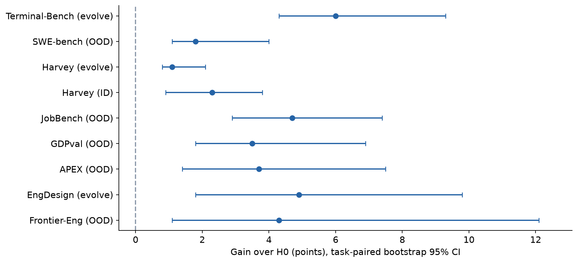
Figure 8. Exact gain and interval endpoints from Table 6. These are paired task-bootstrap intervals for evaluated harnesses; they are not confidence intervals over an unlimited population of evolutionary searches.

All reported intervals lie above zero. SWE-bench’s 1.8-point estimate has interval [1.1, 4.0]; Frontier-Eng’s 4.3-point estimate has a much wider [1.1, 12.1]. The latter is consistent with positive improvement but leaves substantial uncertainty about magnitude. A positive interval across a benchmark collection does not establish performance on every task family or protect against a new domain with a different failure mode.

Intervals on evolve-set gains are additionally conditioned on a harness selected using those tasks. A conventional task bootstrap does not undo adaptive selection. Even on held-out tasks, these intervals describe variation within the observed benchmark, not uncertainty over which future benchmark someone might choose. The protocol is considerably more informative than a single score, but it should not carry claims beyond that scope.

9.2 Two repetitions are useful, but still two

The authors repeat each main evolution run with changed proposer randomness. Both resulting harnesses improve all nine splits relative to the base. Workspace OOD average is 43.6 in the first run and 43.7 in the second. The largest split difference is 1.8 points on Terminal-Bench; the other eight differ by at most 0.6.

This directly addresses the worry that one fortunate proposal sequence produced the whole result. It does not estimate the tail probability of a harmful search, and two trajectories are insufficient to conclude generally that search variance is smaller than evaluation variance. The latter is a reasonable description of the observed pair, not a stable variance-component estimate.

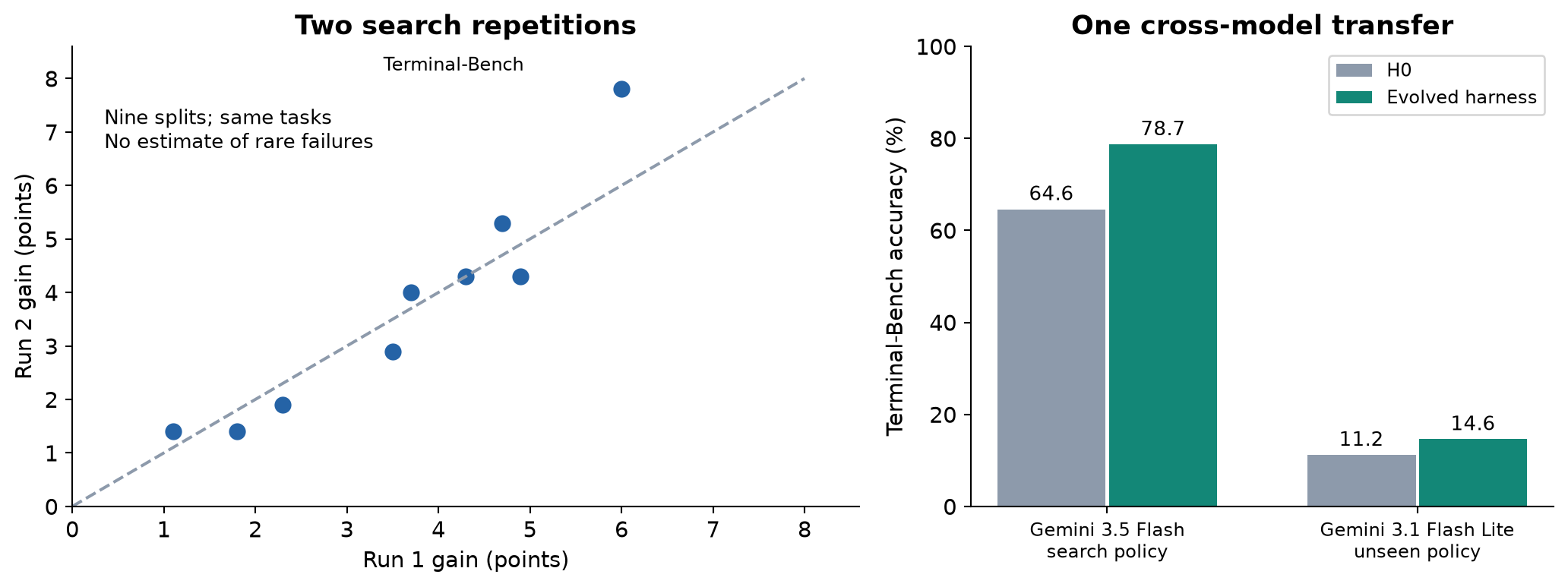
Figure 9. Left: gains from the two searches in Table 7, with the diagonal indicating equality. Right: Table 4’s one unchanged harness transferred from Gemini 3.5 Flash to Gemini 3.1 Flash Lite. These are different kinds of robustness tests.

The paper also performs independent coding searches with Claude Opus 4.8 and Gemini 3.5 Flash. Their OOD SWE-bench gains are 1.8 and 2.2 points, respectively. That tests whether the method can work with more than one fixed policy. A separate experiment runs the Gemini-evolved harness unchanged with Gemini 3.1 Flash Lite: Terminal-Bench improves from 11.2 to 14.6. That tests one particular cross-model transfer. It is neither a new OOD task test nor evidence of universal compatibility across models.

The 30.4% relative improvement for the smaller policy comes from $3.4/11.2$. Its absolute score remains 14.6. Both the denominator and absolute performance matter when judging usefulness. A small base score can make a modest absolute change sound much larger when expressed only as a relative percentage.

10. Design choices and where alternatives may be better

Decision	Why it can help	Alternative	Failure boundary
Decreasing edit budget	Improves attribution late in search	Fixed single edits	Coordinated repairs may require several changes
Full measured history	Retains negative evidence	Recent-window summaries	Old failures may be obsolete after dependencies change
Best-ever score floor	Blocks accumulated local regressions	Paired re-testing	A lucky high incumbent can anchor an excessive floor
Token-growth gate	Makes extra compute explicit	Cost-matched optimization	Tokens do not capture tool latency or search cost
Novel structural types	Encourages unused mechanisms	Behavioral diversity	Category labels are a coarse proxy for novelty
Pruning proposals	Challenges accumulated machinery	Controlled ablations	Shared candidate credit confounds component utility

The paper’s rules make most sense when task feedback is scarce and candidate evaluations are expensive. They spend less budget on elaborate causal attribution and rely on conservative acceptance plus transfer testing. In a cheap simulator, a larger factorial ablation design might identify useful combinations more reliably. In a changing production environment, a permanent negative-evidence record may need decay or contextualization, because a once-invalid hypothesis can become appropriate after a tool or model update.

A cost-matched baseline is another important alternative. If the initial harness received the same inference budget as the evolved one, perhaps through a generic retry or verification mechanism, how much of RRSI’s improvement would remain? Table 2 shows that RRSI beats more expensive unregularized evolution, which is meaningful. It does not by itself isolate the value of learned mechanism design from the value of allocating extra test-time computation well.

11. Limitations of the evidence

The authors restrict the study to frozen-backbone harness evolution. Jointly training weights and changing the harness would create additional feedback loops and invalidate some simple attribution. The results also cover a limited set of initial architectures, tool environments, and search horizons. Forty rounds of engineering evolution do not establish indefinite self-improvement.

The empirical noise band is a practical tolerance, not a sequential testing guarantee. The critic is a language-model judgment, not an oracle for distributional generalization. Component-level credit is inherited from bundled candidates, and the novelty vocabulary is manually defined. These are reasonable approximations, but their errors can interact: a misattributed gain can preserve a component, alter later proposals, and eventually reinforce a misleading explanation.

Reported execution tokens omit the full search bill. Equal candidate budgets also do not equalize proposer tokens, critic calls, analyst work, or aborted evaluations. Missing within-band weights and domain-guard details limit how precisely the paper alone specifies every decision. The cosine schedule’s endpoint and GDPval’s comparison count add further ambiguities. These are reasons to qualify the operational interpretation, not reasons to invent missing settings.

12. Critical analysis: the useful idea is a burden of evidence

My strongest reading of RRSI is that persistent harness changes should carry a burden of evidence. An edit should explain which failure it addresses, survive a score floor, justify its resource use, and remain useful outside the feedback that created it. This shifts attention from the quantity of proposed improvements to the quality of retained changes. That is a valuable engineering principle even if the particular cosine schedule or novelty categories are later replaced.

The evidence supports the combined procedure more strongly than its regularization analogy. There is no theorem relating the chosen edit count, pruning window, and cost slope to a bound on transfer risk. The observed OOD improvements are the substantive contribution. Calling the three controls $L_0$, $L_1$, and $L_2$ can make the method memorable, but borrowing these names should not import the mathematical guarantees of the corresponding estimators.

There is also an important gap between avoiding blatant leakage and avoiding benchmark adaptation. Appendix F itself notes that prior harnesses need not hard-code task names to fit a rubric or document genre. A semantically general-looking checklist can still be specialized. The held-out results are therefore essential evidence; the critic cannot replace them. If researchers repeatedly redesign the algorithm after seeing those held-out results, a fresh outer test collection becomes necessary for the next round of claims.

Several follow-up experiments would sharpen the conclusions. First, hold final inference cost approximately fixed and compare evolved mechanisms with generic additional verification. Second, run multiple independently randomized evolve splits and substantially more search seeds, reporting both average transfer and worst-case regressions. Third, separate the acceptance components and measure their interactions rather than only removing the entire group. Fourth, calibrate the critic on both deliberately specific changes and suspicious-looking but reusable changes. Fifth, test a longer horizon in which the initially untried component set has been exhausted.

These are proposals, not experiments performed for this review. Their purpose is to distinguish three explanations that current aggregate scores partly mix: better mechanisms, better compute allocation, and a favorable match between regularization choices and these benchmarks. RRSI provides encouraging evidence for the first while clearly improving the second relative to unregularized search. Establishing how often both survive new environments remains the harder question.

13. Conclusion

RRSI offers a concrete answer to when an agent should keep a self-proposed change: only after the change survives restrictions on specificity, stability, and resource growth, informed by a history that includes failures. Its strongest result is not a large increase on the evolve tasks. It is the preservation of useful gains on held-out tasks while accepting less evolve-set improvement than several baselines.

The practical lesson is to treat a self-evolving harness as an adaptive experiment with a finite evidence budget. Sparse edits improve interpretability, conservative selection restrains drift, and transfer tests reveal whether the resulting behavior travels. None alone proves generalization. Together, as reported in this paper, they produce a more convincing case for improvement than a rising search score would.

References and reading pointers

1. Peng Xia et al. RRSI: Regularized Recursive Self-Improvement of Agent Harnesses, v3. Method: Section 3 and Appendix D; benchmark definitions: Appendix B; hyperparameters and uncertainty: Appendix E; qualitative evidence: Appendix F.
2. RRSI authors’ project. A companion resource; numerical comparisons in this review use the versioned paper’s tables.
3. Official code resource. Provided as a resource entry.