SpecScale: Making Speculative Reasoning Search Work Under Serving Load

Review date: 2026-10-22
Paper: Taming Speculative Search for Test-Time Scaling in LLM Serving
Authors: Jinwoo Jeong, Woohyung Choi, Myeongjae Jeon, Jeongseob Ahn
Version: arXiv:2609.39334v1, 2026-09-30
Primary sources: versioned paper, full PDF

1. Why doing useful work early can still make a server slower

Imagine a reasoning service that explores four solutions to a mathematics problem. One candidate finishes its next step quickly; another is still producing a long derivation. A synchronous search waits for all four steps, scores them, and decides which candidates may continue. Speculative search lets the early finisher start its next branches immediately. For a single request, this looks like an obvious way to recover otherwise idle time.

The difficulty is that a busy server does not lack work. Other requests can already occupy the GPU. An early branch that is later discarded competes with useful work from those requests, consumes key-value cache space, and creates additional verification calls. The service may remove a barrier inside one request while making the shared queue longer for everyone. The paper’s central contribution is to treat this as a serving problem, with computation, verification, and memory coupled together.

SpecScale combines three techniques: early pruning (EP) removes descendants of candidates that can no longer survive selection; computation deduplication (CD) represents identical token prefixes once while retaining multiple independent sampling opportunities; lazy verification (LV) delays some scoring calls so that a process reward model can handle them in more efficient batches. These are complementary, but they are not interchangeable. Pruning changes how long losing branches remain alive, deduplication changes the physical work needed to represent a set of paths, and verification scheduling changes when the system learns which paths are losing.

The strongest reported throughput comparison is 2.18x over naive speculation and 1.87x over the evaluated FastTTS configuration. Those are not gains over the non-speculative baseline. In the corresponding eight-beam Qwen2.5-7B MATH setting, the labeled values are 466, 214, 249, and 327 output tokens/s for full SpecScale, naive speculation, FastTTS, and non-speculative search respectively. The gain over non-speculative search is therefore about 1.43x. Keeping the denominator visible is essential to understanding the result.

This review covers all 14 pages of v1, including the experimental details and references; that version has no separate appendix. Figures 1, 3, and 9 reproduce selected original panels. The other figures are explicitly labeled numerical redrawings or analytical illustrations. The probability, work, and queueing derivations below are explanatory analysis rather than additional measured results.

1.1 What is being speculated?

Here the speculative unit is a future reasoning branch whose parent has not yet survived a search decision. It is not necessarily a sequence of draft tokens checked against a target language model. The generator creates reasoning candidates and a process reward model, or PRM, scores their steps. Starting the next step early is useful only if that branch eventually belongs to the retained search frontier.

This also separates SpecScale from SpecReason. SpecReason asks whether a smaller model can supply a reasoning step that a larger model considers acceptable. SpecScale asks how to serve a branching search efficiently when generation and PRM evaluation share resources. Both operate above individual token acceptance, but their correctness questions differ: semantic acceptability in one case, search selection and redundant execution in the other.

2. Prerequisites: the search, the verifier, and the GPU

2.1 Beam size is a logical budget

The paper describes a search with beam size $N$, expansion width $M$, and $k=N/M$ retained candidates. At a selection boundary, $N$ candidate steps are evaluated; the best $k$ are retained and each is expanded into $M$ continuations. Thus the next frontier again contains $N$ logical candidates. For example, $N=8$ and $M=4$ means retaining two parents and exploring four continuations from each.

This terminology matters because the number of active physical sequences can exceed the beam size under speculation. Candidates from several unresolved levels can coexist. Conversely, deduplication can make the number of physical sequences smaller than the number of logical paths. A statement about eight beams therefore does not directly specify the actual decode batch size or the amount of allocated KV memory.

A PRM supplies a score for a completed reasoning step in its context. The paper uses scores in $[0,1]$. A score of one is the model’s maximum output, not a certificate that a mathematical argument is correct. Search quality depends on how these scores rank useful continuations. The paper also describes final answer selection using a weighted sum of step scores; it does not provide enough detail to reconstruct every weighting choice from that phrase alone.

2.2 Verification is a different computational phase

Autoregressive decoding adds tokens iteratively and repeatedly reads model weights and cached attention state. In this setting, PRM verification is a prefill-only forward computation over the reasoning context to be scored. It does not generate an autoregressive critique. Its preferred batch shape can therefore differ substantially from the generator’s preferred batch shape.

On a single GPU, invoking verification interrupts opportunities to advance generation. A small verification batch may pay scheduling and launch costs without using the GPU efficiently. Making every completed candidate trigger an immediate scoring call can fragment a workload that would otherwise have been processed in larger batches. The paper reports that naive speculation increases the number of verification invocations by roughly two to three times in its motivating comparison.

Continuous batching and prefix KV sharing help, but neither makes this conflict disappear. Continuous batching fills decode iterations with available sequences. Prefix sharing avoids storing or recomputing some existing attention history. Neither automatically merges independent forward computations over the same current prefix, and neither decides how long a completed step should wait for its PRM score.

2.3 Three different objectives

A throughput experiment asks how much work a saturated system can finish per unit time. A latency experiment asks how long a request spends from arrival to completion. Answer accuracy asks whether the result is correct. These objectives interact, and the paper measures them under different setups.

In particular, its normalized output latency is end-to-end latency divided by the number of generated output tokens. This is not inter-token latency, time to first token, or a percentile of raw request completion time. A system can change the denominator by changing the amount of generated work. A lower normalized value is informative, but cannot by itself establish a better user-visible tail latency at fixed answer quality.

3. A work-and-dependency model for the speculation trade-off

Consider an explanatory model with $W$ units of useful GPU work and a dependency-limited critical path of length $S$. Let $C$ be the effective processing capacity in matching work units per second. A necessary lower bound is

$$T \geq \max\left(\frac{W}{C},S\right). \tag{1}$$

This is a conceptual lower bound, not a performance model fitted to the paper. Real GPUs have phase-dependent capacity, memory constraints, and scheduling overhead. Still, it clarifies the opportunity: speculation may shorten $S$ by overlapping a future step with an unresolved current step, while adding wasted work $W_{\mathrm{waste}}$.

After speculation, a corresponding lower bound is

$$T_{\mathrm{spec}} \geq \max\left(\frac{W+W_{\mathrm{waste}}}{C},S_{\mathrm{spec}}\right), \qquad S_{\mathrm{spec}}\leq S\ \text{in the intended overlap scenario}. \tag{2}$$

The inequality on the critical path describes the intended dependency overlap, not a guarantee about elapsed time under resource contention. If the original request is dominated by $S$, some extra work can be worthwhile. If the server is already dominated by total work divided by capacity, that extra work is a direct liability. This is why results from a single active request can reverse as concurrency increases.

There is a second amplification mechanism. Suppose a losing branch generates at rate $r$ tokens/s and its rejection is learned $d$ seconds later. Its avoidable extra generation is approximately $rd$ tokens, before accounting for descendants. If speculative expansion creates descendants, the total waste can grow faster than this one-branch estimate. Verification delay therefore determines not only latency but also how much invalid work remains in flight.

The paper’s motivating experiments fit this picture. Waiting between steps accounts for a substantial fraction of single-request execution, with reported medians around 20-55% across configurations. Yet naive speculation creates more active candidates and becomes less attractive as concurrency rises. The key engineering question is not whether waiting exists, but whether eliminating that waiting improves the use of the shared resource.

4. Early pruning: one strict argument and one shortcut

4.1 The order-statistic argument

Fix one selection round and assume each candidate’s completed-step score is immutable. Let $V_t$ be the set of candidates already verified at time $t$. Once at least $k$ candidates have been scored, define the current threshold as the $k$-th highest verified score:

$$\tau_t=\operatorname{kthmax}\{s_i:i\in V_t\}. \tag{3}$$

When additional scores arrive, the set grows. Adding elements cannot lower the $k$-th largest value, so

$$V_t\subseteq V_{t+1} \quad\Longrightarrow\quad \tau_{t+1}\geq\tau_t. \tag{4}$$

Now consider a verified candidate $j$ with $s_j<\tau_t$. At least $k$ verified candidates already have strictly higher scores. Those candidates remain part of the final comparison for this round, regardless of the scores of candidates not yet verified. Therefore $j$ cannot enter the final top-$k$. Any speculative descendants of $j$ are unnecessary for this search decision and can be canceled.

The strict inequality is doing real work. A candidate with a score equal to the threshold may survive under the search’s tie-breaking rule. Likewise, an unverified candidate cannot be pruned simply because an ancestor had a low score: the proof concerns the score used at the present selection boundary, not a monotonicity claim about future reasoning quality. Neither a confidence estimate nor a predicted score is enough to substitute for the verified ordering in this argument.

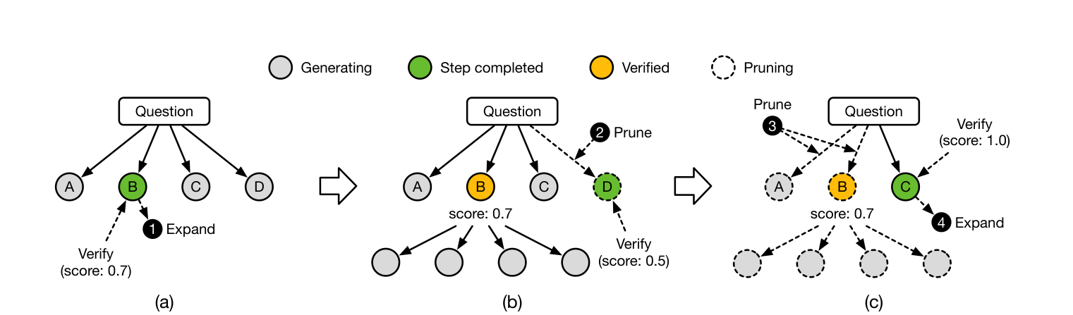
Figure 1. Original Figure 8 from v1, page 6, with $N=M=4$ and $k=1$. Candidate B receives 0.7, D receives 0.5 and is pruned, and C later receives 1.0. The final panel also uses the perfect-score shortcut discussed below.

4.2 A small proof example

Suppose $k=2$ and the first verified scores are 0.80 and 0.50. The threshold is 0.50. A candidate scored at 0.45 is already unable to survive. If later scores are 0.62, 0.74, and 0.40, the threshold rises first to 0.62 and then to 0.74, before staying there. Nothing about the final low score can restore the 0.45 candidate.

Notice what this proof does not require: the PRM need not be well calibrated, and a score of 0.80 need not correspond to an 80% chance of correctness. The pruning is exact relative to this fixed PRM ranking rule. It can faithfully preserve the choices of a poor search policy. Algorithmic equivalence and solution quality are separate properties.

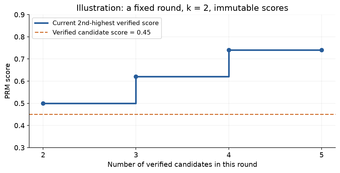
Figure 2. An illustrative trace for $k=2$, constructed for the proof rather than measured from a run. A score below the current threshold cannot recover a place in the top two as more candidates are verified.

4.3 Why a perfect score is different

SpecScale also finalizes selection when $k$ candidates have achieved the maximum score of 1.0. No unseen candidate can have a numerically higher score. However, unseen candidates can have the same score, and the ordinary search might choose different candidates after applying its tie-breaking rule. The paper explicitly acknowledges this distinction in its answer-quality discussion.

For a counterexample, let $k=1$. Candidate A finishes first with score 1.0. Candidate B would finish later with score 1.0 and would win the baseline’s deterministic tie-break. Early completion selects A and cancels B. The score of the selected parent is unchanged, but the selected reasoning history is different. Later expansions and final answers can consequently differ as well.

The shortcut is especially effective when the PRM produces many perfect scores. The paper observes more such scores for its Qwen configuration than for its Llama configuration. That distribution is an operational property of the particular generator-verifier pair. A verifier whose outputs rarely reach the exact maximum offers fewer opportunities for this shortcut, even if its ranking quality is excellent.

4.4 Algorithm 1: selection-aware cancellation

The following numbered pseudocode makes the two policies explicit. It is an explanatory formulation of the paper’s method; the choice of data structures is not a claim about a particular implementation.

Algorithm 1. Process a verified score within one search round
Input: candidate c, score s(c), retained count k, verified set V
1. Insert c and its immutable score into V.
2. If |V| >= k, compute the k-th largest verified score tau.
3. Cancel every verified candidate j with s(j) < tau,
   including its speculative descendants for this round.
4. Preserve candidates tied at tau until the tie policy resolves them.
5. Optional perfect-score shortcut:
   if at least k candidates in V have score 1.0,
   select k of them using the shortcut's tie policy;
   cancel the remaining candidates and close this round.
6. Otherwise, close the round after all required scores arrive,
   applying the baseline selection and tie policy.
7. Expand retained parents and release only unreferenced state.

Step 7 is a conceptual memory requirement: canceling a logical path does not imply that all its prefix storage is private. Other paths can still reference shared state. This becomes particularly important once deduplication is introduced. The attractive simplicity of the ranking proof should not hide the fact that cancellation, sampling multiplicity, and shared prefix ownership must describe the same logical search.

5. Computation deduplication: share logits, keep independent draws

5.1 A physical sequence can represent several paths

Suppose four logical candidates currently have exactly the same token prefix. Under the same model state and sampling settings, the next-token distribution is the same for all four. Executing four identical model forward passes is unnecessary: one pass can compute the logits, followed by four independent samples from the resulting distribution.

If three samples choose one token and the fourth chooses another, the next frontier needs two physical prefixes, with multiplicities three and one. The paper calls the number of logical paths represented by a physical sequence its potential size. At the next iteration, the size-three sequence again performs one forward pass and takes three independent samples. Branches are materialized only when their token histories diverge.

The word independent is crucial. Sampling one token and copying it four times would artificially correlate the paths and destroy search diversity. Sharing a deterministic computation of the distribution does not require sharing the random outcome. Computation deduplication relies on that separation.

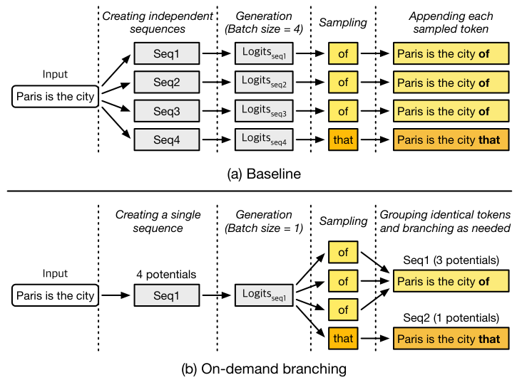
Figure 3. Original Figure 10 from v1, page 6. Four samples from the same logits produce three instances of “of” and one of “that.” The next physical frontier has two prefixes, but still represents four logical paths.

5.2 The multinomial view

Let a prefix induce a categorical next-token distribution $p_v$, and let $m$ logical paths share that prefix. The probability of a particular vector of token counts $(n_v)_v$, where $\sum_v n_v=m$, is

$$\Pr\{(n_v)_v\} =\frac{m!}{\prod_v n_v!}\prod_v p_v^{n_v}. \tag{5}$$

This is exactly the count distribution obtained by taking $m$ independent samples. Grouping the samples after drawing them changes their representation, not this distribution. Conditional on a group’s shared prefix, the same argument applies at the next token. Repeating it gives a natural induction argument for representing independent trajectories with grouped prefixes.

There are assumptions behind that reasoning. The paths must truly share their complete conditioning state, including the token history and relevant sampling configuration. Token-level penalties or constraints that differ across logical candidates must not be ignored. If later selection depends on candidate identity rather than only score and token history, those identities must remain meaningful even when the computation is grouped. These are semantic conditions for the argument, not evidence that the paper tested every possible sampler.

The proof also does not mean that an entire physical execution is bitwise identical to a baseline. Different batch shapes can affect floating-point arithmetic and random-number ordering. The useful claim is about the intended probabilistic computation: compute the same conditional distribution and retain the prescribed number of independent draws. It is stronger and more precise than saying that duplicated text merely “looks redundant.”

5.3 How much branching should we expect?

Define $I_v=1$ if token $v$ appears in at least one of the $m$ samples, and zero otherwise. The number of distinct next-token prefixes is $U=\sum_v I_v$. A token is absent with probability $(1-p_v)^m$, so linearity of expectation gives

$$\mathbb{E}[U] =\sum_v\mathbb{E}[I_v] =\sum_v\left[1-(1-p_v)^m\right]. \tag{6}$$

For a concrete teaching example, take two tokens with probabilities 0.75 and 0.25 and let $m=4$. Then

$$\mathbb{E}[U] =\left(1-0.25^4\right)+\left(1-0.75^4\right) =1.6796875. \tag{7}$$

Four logical continuations therefore produce about 1.68 distinct next-token prefixes in expectation. The ratio $4/1.6796875\approx2.38$ illustrates a potential reduction in the number of next-prefix computations. It is not a predicted 2.38x wall-clock speedup. Sampling, grouping, kernel shape, available batch work, and later divergence all affect elapsed time.

When the distribution is diffuse and $m$ is small relative to the effective vocabulary, most draws differ and $U$ approaches $m$. When probability mass is concentrated, many draws collide and physical work can be shared. The paper’s measurements report roughly 25-50% common tokens across candidates in the studied workloads at temperature 0.8. That empirical overlap supports the mechanism, but the overlap ratio alone is not a sufficient performance prediction.

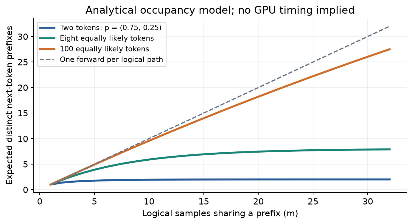
Figure 4. Reader-derived occupancy curves from Equation (6), using the distributions named in the legend. These are analytical examples, not model measurements. Diffuse distributions leave less redundancy to remove.

5.4 Algorithm 2: on-demand physical branching

Algorithm 2. Advance a group of identical logical prefixes
Input: shared prefix x, logical members C with |C| = m
1. Check that members share the same conditional distribution.
2. Evaluate the generator once on the physical prefix x.
3. Form the next-token distribution using the sampling settings.
4. Draw m independent next tokens, one for each logical member.
5. Partition C by the token selected in step 4.
6. For each nonempty partition C_v, create or retain prefix x + v;
   associate its members and multiplicity |C_v| with that prefix.
7. Continue each distinct prefix once in the next decode iteration.
8. Keep selection, termination, and cancellation consistent with
   the logical members represented by each physical prefix.

The paper groups sampling work by potential size to handle the different sample counts. This detail explains why deduplication is more than a cache lookup. It reorganizes the mapping between a batch of physical model inputs and the logical trajectories that those inputs represent.

5.5 Why prefix caching is not enough

Ordinary prefix KV sharing can let four candidates reference the same stored history. They can nevertheless remain four active decode inputs, each producing the same next-token logits. CD removes those duplicate forward computations while retaining four draws. Conversely, if the four candidates already differ by one token, common-prefix KV sharing can still save memory even when their current logits can no longer be merged.

The techniques address different redundancy. This distinction also suggests an important evaluation control: non-speculative search can benefit from CD too. Comparing full SpecScale only with non-speculative search without CD mixes the benefit of speculation management with a more general improvement in multi-path generation. A matched non-speculative-plus-CD baseline would clarify how much residual value comes specifically from executing ahead of selection.

6. Lazy verification: pay less per score, learn the score later

6.1 Why immediate feedback is not always cheapest

A completed reasoning step is ready for scoring, but the most efficient time to score it may be slightly later, together with other completed steps. The paper profiles PRM throughput and finds saturation around 2,048 input tokens in the relevant batch configuration on its A100. LV uses this observation to aggregate verification tasks across requests.

The policy has three alternative triggers. Verification runs when the accumulated input-token volume reaches the profiled threshold; when all siblings sharing a parent have completed their steps; or when an individual task has been deferred too many times. The paper uses an empirically chosen maximum deferral count of six. These conditions are joined by “or”: a sibling group can force progress without filling the token threshold.

A deferral count is not a duration in milliseconds. Six opportunities to postpone a task can represent different elapsed time under different batch lengths or competing work. The count cap provides a progress mechanism, but it does not establish a hard wall-clock response-time bound. This distinction matters when moving from a benchmark to a service with a strict latency requirement.

6.2 A simple amortization model

For intuition, let verification of $B$ input-token units cost $a+bB$, where $a$ is fixed overhead and $b$ is marginal cost. Then throughput in this simplified model is

$$q(B)=\frac{B}{a+bB}. \tag{8}$$

Differentiating gives

$$\frac{dq}{dB}=\frac{a}{(a+bB)^2}>0, \qquad\lim_{B\to\infty}q(B)=\frac{1}{b}. \tag{9}$$

Bigger batches amortize the fixed cost but deliver diminishing returns. Real PRM execution has more complicated shape dependence and memory behavior, so the paper profiles it rather than deriving an optimum from this toy model.

Now suppose input-token work arrives at a smooth rate $\lambda_v$. A threshold-only batch of size $B$ takes approximately $B/\lambda_v$ time to fill. Under an even-arrival approximation, the average accumulation wait is roughly

$$\mathbb{E}[D]\approx\frac{B}{2\lambda_v}. \tag{10}$$

Equation (10) deliberately ignores the other two triggers, burstiness, and discrete request sizes. Its role is to expose the competing cost: larger batches can improve GPU efficiency while delaying the information used to cancel losing branches. Combining this with the earlier $rd$ estimate shows why a throughput-optimal verifier batch in isolation need not be optimal for the complete search.

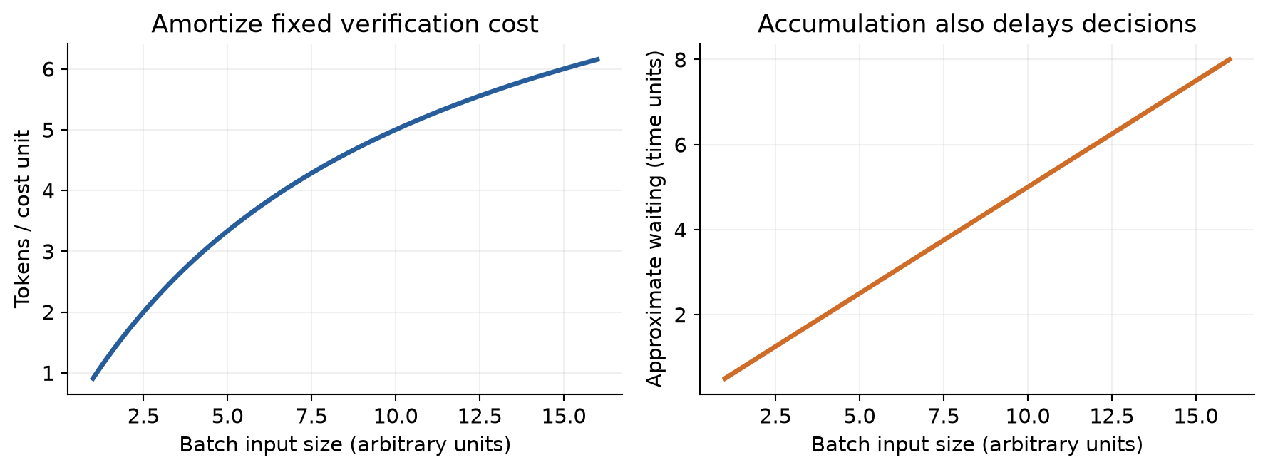
Figure 5. A hypothetical illustration with $a=1$, $b=0.1$, and arrival rate one input unit per time unit. Units are arbitrary. The curves are not the paper’s PRM profile and do not imply that the actual system follows a linear cost model.

6.3 Algorithm 3: a progress-aware verification queue

Algorithm 3. Decide whether to run a PRM batch
Input: pending completed steps Q, token threshold B_max,
       deferral limit d_max, search sibling relationships
1. Add newly completed steps to Q with their scoring contexts.
2. Count the total verification input-token volume in Q.
3. Check whether any sibling group has fully completed its step.
4. Check whether a pending task has reached its deferral limit.
5. If the token threshold, sibling condition, or count limit fires,
   run a verification batch including eligible pending tasks.
6. Deliver scores to the appropriate selection rounds;
   apply Algorithm 1 and remove canceled pending work.
7. Otherwise retain tasks and update their deferral bookkeeping.
8. Repeat while generation and search continue.

This pseudocode expresses the policy, not a specific scheduler API. Exact queue accounting and inclusion rules affect batch composition. In particular, counting verification input tokens is different from counting generated output tokens, because each scoring context can include substantial prior reasoning and formatting.

The sensitivity experiment gives a practical warning against treating 2,048 as a universal constant. The paper varies the threshold from 256 to 4,096 in the stated study and finds the best reported operating point at 2,048. Increasing it to 4,096 reduces throughput below the EP+CD baseline without LV. The gain from aggregation has a limit, after which delayed pruning and other waiting costs dominate.

7. How the three mechanisms interact

It is tempting to read EP, CD, and LV as three independent speedup multipliers. That is not a good mental model. They change each other’s operating conditions. Early pruning reduces the number of live speculative paths; CD reduces the number of physical decode inputs for the surviving logical paths; LV changes when the information needed for pruning becomes available.

Consider a candidate that has completed a step but has not yet received a PRM score. Its speculative descendants may continue decoding. Some descendants can share physical prefixes with other logical paths. A later low score should cancel only the descendants that are logically attached to this losing parent. Removing shared state too aggressively would affect unrelated paths; retaining it indefinitely would erase the memory benefit. The search frontier, the physical batch, and prefix ownership therefore need coordinated bookkeeping.

There is also a batching interaction. CD can reduce the number of generator inputs, which may improve efficiency by removing redundant work but can also make a small workload less able to occupy the GPU. The paper finds different incremental benefits for different model sizes. A smaller model with unused compute capacity does not necessarily get the same elapsed-time gain from removing one duplicate path as a larger model in a constrained batch.

Finally, a score can be valuable before it is cheap. A nearly full KV cache or a rapidly expanding set of uncertain branches increases the cost of postponing verification. The paper’s fixed triggers are a practical design, but the broader policy question is state dependent: how much invalid work or memory pressure is the system willing to tolerate in exchange for a more efficient PRM batch? This is a natural place for future adaptive scheduling, provided its control overhead remains small.

8. What the experiments actually compare

The main platform is one NVIDIA A100 with 80 GB of memory and an Intel Xeon Gold 6326 host. The paper specifies PyTorch 2.9 and CUDA 12.8, and uses a shared serving framework with continuous batching, paged attention, prefix KV sharing, and FlashInfer. These common mechanisms matter because otherwise a speedup could simply reflect a stronger underlying serving engine.

The generator-verifier pairs include Qwen2.5-3B and Qwen2.5-7B with Qwen2.5-Math-PRM-7B, plus Llama3.2-3B and Llama3.1-8B with a Llama3.1-8B PRM. The main workloads are 1,000 sampled GSM8K problems, MATH-500, and OlympiadBench as described in the paper. Search uses beam sizes four and eight, expansion width four, at most 40 expansion steps, and temperature 0.8. The main maximum concurrency is 32; separate experiments vary concurrency and beam size.

For saturated throughput, requests are issued together. For serving behavior, the paper uses Poisson request arrivals and measures normalized end-to-end output latency as the request rate increases. The former tests capacity under abundant work; the latter exposes queueing effects. A claim from one setup should not silently be substituted for a claim from the other.

The FastTTS comparison needs qualification. The authors reimplement its speculative candidate selection and lookahead verification inside their common framework, explaining that the released version used in their comparison supports batch size one. They omit preemptible scheduling and dynamic prefix-aware scheduling, which they describe as targeting constrained-device settings. They report a batch-one consistency check with Qwen2.5-7B on MATH across several beam sizes, while omitting detailed numbers for that check.

This is a reasonable attempt to compare relevant mechanisms under common batching support. It is nevertheless a comparison against the evaluated configuration, not proof that every FastTTS deployment would have the same performance gap. Reading the headline with that qualifier preserves what the experiment establishes without dismissing the engineering work needed to construct the comparison.

9. Throughput and ablations: keep the denominator in view

Figure 6 redraws the paper’s labeled MATH bars for Qwen2.5-7B. At four beams, full SpecScale reaches 786 output tokens/s compared with 558 for non-speculative search. At eight beams, the corresponding values are 466 and 327. Throughput decreases with the larger search budget for all these configurations, even though the relative benefit remains substantial.

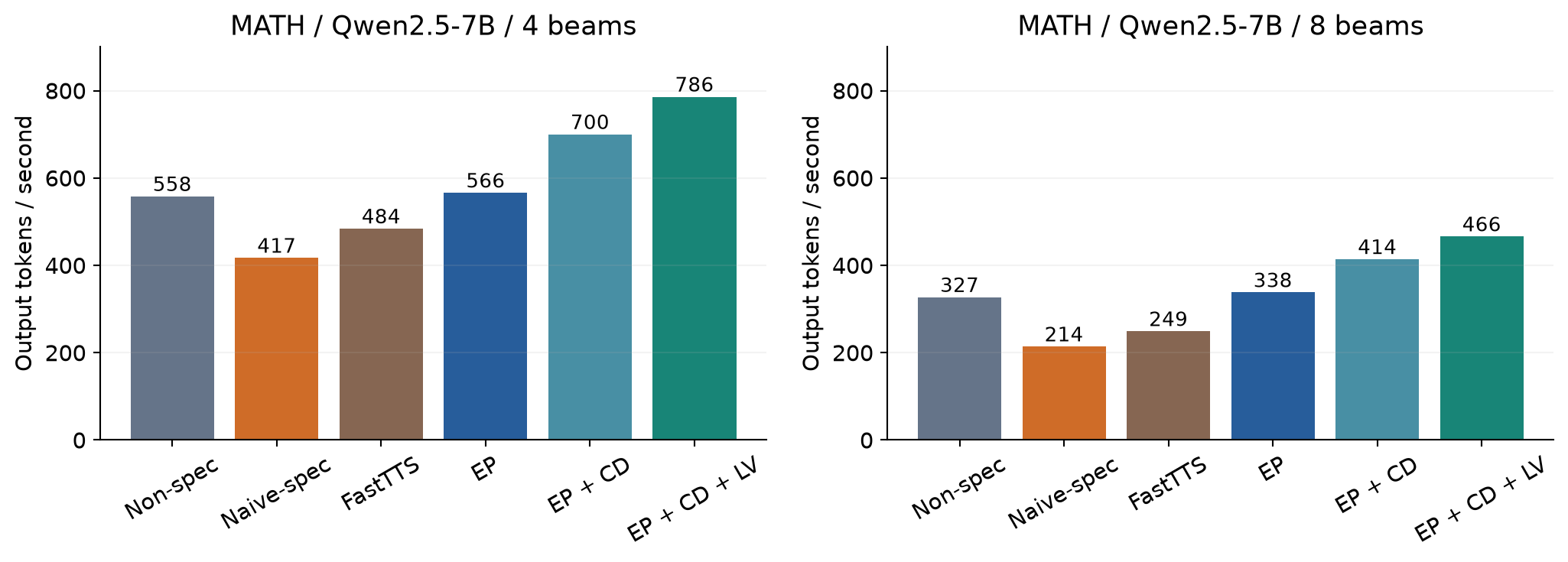
Figure 6. Redrawn from the labeled bars of original Figure 13(b), v1 page 9. EP, CD, and LV are added cumulatively. The model pair is Qwen2.5-7B-Instruct and Qwen2.5-Math-PRM-7B on one A100 80 GB.

For the eight-beam case, the arithmetic is

$$\frac{466}{214}\approx2.18,\qquad \frac{466}{249}\approx1.87,\qquad \frac{466}{327}\approx1.43. \tag{11}$$

The first two comparisons recover the paper’s headline against naive speculation and FastTTS; the third is the gain over non-speculative search. These ratios are compatible because the baselines have very different costs. Naive speculation is only $214/327\approx0.65$ of non-speculative throughput in this setting. Much of the full system’s value comes from repairing that regression and then going beyond the original baseline.

The ablation also shows that EP alone is not the whole result. At eight beams, throughput moves from 338 with EP to 414 with EP+CD and 466 with all three. The incremental CD factor is $414/338\approx1.22$, while the LV factor is $466/414\approx1.13$. These factors describe that configuration; they should not be generalized to every model and workload.

For Qwen2.5-3B on MATH with eight beams, the paper reports 317, 375, 411, and 479 output tokens/s for non-speculative search, EP, EP+CD, and the full system. CD adds about 1.10x over EP there. The different increment is consistent with the paper’s explanation that redundant computation has a different opportunity cost for different generator sizes.

The Llama results are particularly useful because they prevent an overly simple story. In some MATH and Olympiad configurations, EP alone remains below the non-speculative baseline. The authors connect this to fewer perfect PRM scores and hence fewer opportunities to finish a selection round immediately. CD and LV are needed to produce the full benefit. The method’s success depends on the joint distribution of branch overlap, completion times, and verifier scores, not just the existence of a search tree.

10. Accuracy, latency, and memory require separate readings

10.1 Accuracy is comparable, not identical

Table 2 evaluates Qwen2.5-3B search accuracy. With four beams, the non-speculative results are 92.99% on GSM8K, 74.03% on MATH-500, and 27.18% on OlympiadBench. Full SpecScale gives 93.49%, 75.43%, and 27.94%. With eight beams, the baseline gives 94.70%, 76.24%, and 30.40%, while the full system gives 94.09%, 76.82%, and 31.48%.

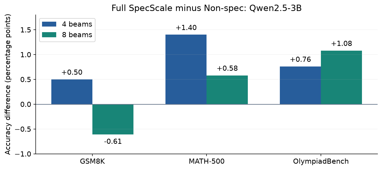
Figure 7. Full-system minus non-speculative differences from Table 2, in percentage points. The evaluated generator is Qwen2.5-3B. These are point estimates; the table does not supply confidence intervals or run-to-run variability.

These results support the paper’s description of comparable answer quality on the measured tasks. They do not demonstrate exact answer preservation. In particular, the GSM8K eight-beam difference is -0.61 percentage points, while the MATH four-beam difference is +1.40 points. A system with approximate tie handling and stochastic sampling can move in either direction.

The intermediate ablations reinforce that point. EP alone changes MATH eight-beam accuracy from 76.24% to 79.21%, a +2.97-point difference, while its Olympiad eight-beam difference is -1.01 points. This is not a monotonic accuracy ladder as more optimizations are added. Without paired seeds and uncertainty estimates, it is difficult to disentangle changed candidate choices, stochastic variation, and any interaction with the search budget.

The quality table also covers a different generator size from the headline Qwen2.5-7B throughput case. That does not invalidate either result, but it limits how tightly they can be joined into a claim about a single quality-throughput operating point. A matched table covering the exact same model, budget, and workload for both metrics would make that interpretation stronger.

10.2 Less waiting is not the final objective

Figure 15 breaks down time for Qwen2.5-7B on MATH with four beams. In the non-speculative baseline, generation occupies 65.0% of total time and verification 27.8%. Under naive speculation, these components rise to 76.2% and 43.8% of the baseline’s total time. Those numbers use a common reference denominator; they are not percentages that must sum to 100 within each method.

With EP+CD, generation and verification account for 46.7% and 32.8% of baseline time. Adding LV changes them to 48.9% and 20.5%. Generation time increases slightly, while verification time drops substantially. This is precisely the trade-off expected when the system waits longer to obtain pruning information but runs the verifier more efficiently.

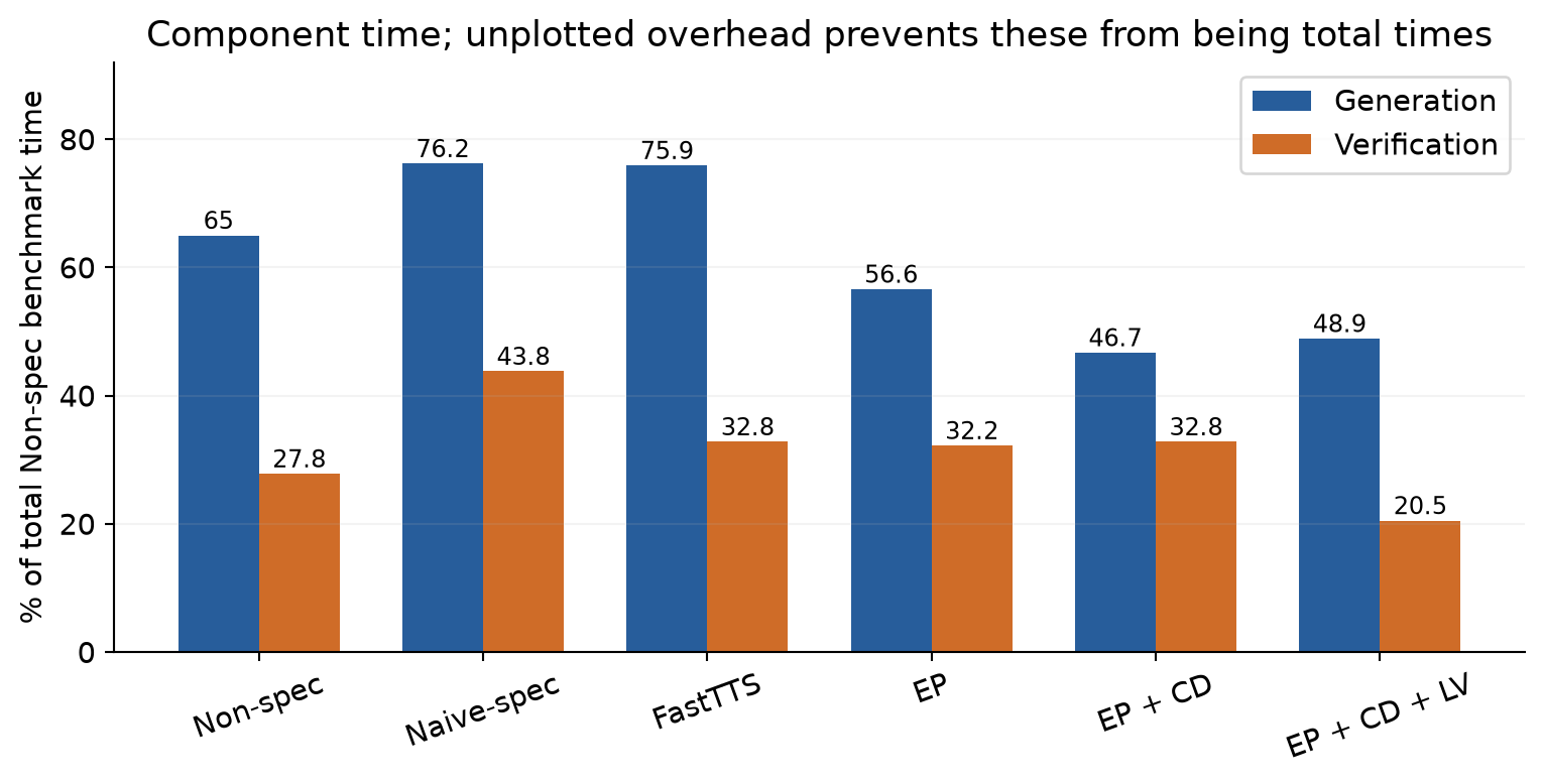
Figure 8. Exact labeled generation and verification components from original Figure 15(a), page 11. Miscellaneous overhead is not plotted, so adding these bars does not recover the full normalized execution time.

The paper separately discusses residual costs such as tokenization for the verifier’s prompt format. Tokenization is reported to account for about 40% of an approximately 7% “other” component in the baseline. Even after improving the GPU phases, host-side work can become a meaningful fraction of the remaining runtime. This is another reason to avoid predicting end-to-end speedup from a single kernel-level saving.

The threshold sensitivity plot tells the same story from a different angle. In the Qwen2.5-3B MATH-500 study, 2,048 tokens produces roughly 1.09x and 1.14x throughput over EP+CD without LV for four and eight beams respectively. At 4,096 tokens, both are below that no-LV baseline. Delaying a score has a measurable opportunity cost; larger verification batches are useful only while their efficiency gain exceeds that cost.

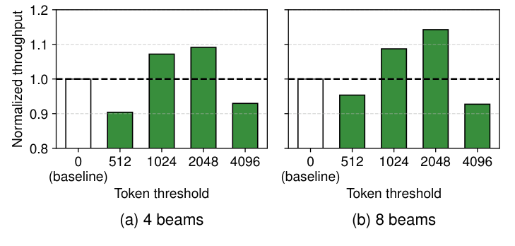
Figure 9. Original Figure 16 from v1, page 11. The dashed reference is EP+CD without lazy verification. The 2,048-token operating point belongs to this hardware, model, and workload study; it is not a portable default established by theory.

10.3 Serving curves and scaling

In the serving plots, full SpecScale sustains higher request rates before normalized latency rises sharply. For the Qwen2.5-7B four-beam case, the paper discusses an operating region around 75 ms per generated output token at approximately 1.6 requests/s for SpecScale, compared with roughly 0.8 requests/s for FastTTS at a similar normalized latency. These are plot-level comparisons, not a measurement of a guaranteed request deadline.

The broader concurrency experiment varies the maximum concurrent requests from 16 to 128. In the four-beam setting, the baseline and FastTTS saturate around 64, while SpecScale continues to benefit over the reported range. Reduced speculative waste and memory use can leave room for more requests, but this observation is still specific to the evaluated single-device workload and admission pattern.

When the beam size reaches 32 in the reported Qwen2.5-7B MATH scaling experiment, normalized latency is approximately 330 ms for non-speculative search and 195 ms for SpecScale, with about 22% lower KV memory. The latency ratio is approximately $330/195\approx1.69$; the reduction relative to the baseline is about 41%. Those are two different ways to describe the same approximate values. Neither should be confused with a 69% latency reduction, and neither establishes an energy saving because energy was not the measured quantity.

11. Limitations and failure boundaries

The workload is PRM-guided mathematical search. The main evidence comes from GSM8K, MATH-500, and OlympiadBench. A tool-using agent with external side effects has additional constraints: speculative actions may not be cancelable, and completing a branch can change the environment observed by other branches. The paper’s benefits should not be transferred directly to such a workflow merely because both involve reasoning trees.

Strict pruning preserves a local ranking decision, not truth. It assumes fixed completed-step scores and a fixed selection round. A search that updates earlier scores, uses diversity penalties, or applies global path constraints may not satisfy the same order-statistic argument. An unseen candidate tied at the threshold also requires a defined tie policy. The perfect-score shortcut explicitly relaxes candidate identity preservation.

Deduplication depends on exact conditional equivalence. Similar text is insufficient. Prefixes with different tokens, hidden conditioning state, or sampling constraints may induce different distributions. If the generator produces highly diverse continuations, little physical work can be merged. Grouping overhead then has less computation to offset it.

A verifier is part of the performance workload. Its score distribution determines early-stop opportunities; its input formatting and context length determine prefill cost; its batch curve determines useful aggregation thresholds. Changing the PRM can change all three. Better ranking quality does not automatically mean a more favorable serving profile.

Deferral is bounded by count rather than elapsed time. Under low traffic, unusual branch lengths, or competing long verification work, the count limit is not a documented wall-clock guarantee. The paper’s observed serving curves do not supply a formal fairness or tail-latency bound for every request class.

The hardware evidence is single-GPU. There is no direct experimental basis here for claims about multi-node communication, disaggregated generation and verification, or heterogeneous device placement. A distributed system could make batching easier by pooling work, or more expensive by adding transfer and synchronization overhead. Both are possibilities rather than results of this paper.

The quality uncertainty is not fully quantified. The reported accuracy table gives useful point estimates but no confidence intervals, and it does not match every throughput model configuration. Comparable measured accuracy is a narrower statement than a guaranteed quality-preserving transformation. The paper is most persuasive when its claims are kept at that empirical level.

12. Critical analysis: what would make the evidence more decisive?

12.1 Separate the exact pruning rule from perfect-score termination

I would first compare three policies under paired logical sampling: no early pruning, strict-below-threshold pruning only, and strict pruning plus the perfect-score shortcut. The first comparison isolates cancellation that should preserve the fixed-round top-$k$ result. The second measures the additional benefit and quality effect of ending before ties are fully known.

This matters because arrival order can become an implicit preference. Shorter or faster candidates are more likely to supply the first perfect scores. If reasoning length correlates with difficulty or solution style, the shortcut may favor particular trajectories even when their scores are tied. A useful experiment would report which candidates change, how their lengths differ, and whether the final accuracy effect is stable across seeds. Merely counting perfect scores does not reveal this selection bias.

12.2 Include non-speculative search with deduplication

CD is a general way to reduce repeated computation across identical logical paths. A complete factorial comparison would include non-speculative+CD, speculative+CD, speculative+EP+CD, and the full system, all with the same prefix caching and sampler semantics. This would separate “speculation is useful after controlling its waste” from “multi-path generation was doing duplicate forwards.”

The distinction is practically important. If non-speculative+CD captures much of the gain for a workload with little barrier waiting, it may offer a simpler operating point. If full SpecScale still wins substantially under the same logical search, that strengthens the case for the additional scheduling machinery. The paper’s current ablations explain how its components help the speculative system, but do not fully answer this alternative-design question.

12.3 Measure completed correct answers under a latency budget

A deployment-facing comparison should match the generator, PRM, search budget, and accuracy target, then report raw end-to-end request latency and the number of completed correct answers per unit time. One possible metric is

$$G_{\mathrm{correct}}(L) =\frac{\#\{\text{correct completed requests with latency}\leq L\}} {\text{measurement duration}}. \tag{12}$$

This is a proposed evaluation metric, not one reported in the paper. It avoids treating extra output tokens as useful by definition and makes the latency requirement explicit. It should be accompanied by accuracy, completion rate, and latency percentiles, since a single aggregate can conceal which requests are being delayed or dropped.

For stochastic search, paired evaluation is particularly valuable. Reporting an average over seeds with uncertainty estimates would distinguish a consistent quality-performance improvement from one favorable realization of the sampled paths. The same evaluation should stratify easy and hard problems, because high-overlap, high-perfect-score workloads may benefit disproportionately.

12.4 Adapt the verification threshold to the cost of uncertainty

The observed failure of a 4,096-token threshold suggests a useful control variable: not just pending verifier tokens, but the expected cost of leaving branches unresolved. A candidate surrounded by many active descendants or substantial KV usage has a higher cost of delayed rejection than an isolated candidate with no speculative descendants.

An adaptive design could flush verification when a combination of waiting time, uncertain descendant work, and memory pressure exceeds a budget. It would still retain the sibling completion condition to avoid unnecessary barriers. Such a policy would need a careful comparison against the simple fixed threshold; a complicated predictor that costs more than it saves would defeat the purpose.

I would treat a wall-clock age cap as a separate safeguard from a deferral-count cap. The former relates to a service promise, while the latter relates to scheduler opportunities. Distinguishing them makes both the operational semantics and the evaluation easier to explain.

12.5 The most useful general lesson

The paper is strongest as a study of when information arrives relative to the work that depends on it. A PRM score is valuable because it can stop future computation. Delaying that score may make its own computation cheaper, but also increases the amount of work performed without knowing whether it is useful. Shared-prefix execution reduces that uncertainty cost by making several possible paths cheaper to keep alive.

This framing is more durable than any one throughput multiplier. It suggests measuring the lifetime of losing branches, the physical-to-logical sequence ratio, the distribution of verifier batch sizes, and the memory attached to unresolved decisions. Together, those quantities explain why a policy succeeds or fails as load changes. They also offer a clearer guide for extending the method than assuming that more aggressive speculation is always better.

13. Conclusion

SpecScale makes speculative reasoning search more plausible under serving load by addressing three sources of inefficiency together: losing branches that live too long, identical prefixes that are evaluated repeatedly, and verification calls that are too small to run efficiently. Its throughput and ablation results provide concrete evidence that removing search barriers is insufficient unless the extra work is controlled.

The important qualifications are equally concrete. Strict early pruning has a local order-statistic justification; perfect-score termination can change tied candidate choices. Deduplication shares model computation while preserving independent draws under explicit assumptions. Lazy verification trades immediate knowledge for batch efficiency and has an empirically finite useful range. The measured accuracy is comparable, while exact candidate or answer preservation is not established for the full system.

My takeaway is to optimize the cost of an unresolved search decision, rather than merely the speed at which the next branch can start. SpecScale demonstrates how much that distinction matters on a busy single GPU, and leaves a clear set of questions about matched baselines, tail latency, and adaptive verification for future work.

References

Jeong et al. Taming Speculative Search for Test-Time Scaling in LLM Serving. arXiv:2609.39334v1, 2026-09-30 (PDF).