SpecReason: When Can a Small Model Take the Next Reasoning Step?

Review date: 2026-10-21
Paper: SpecReason: Fast and Accurate Inference-Time Compute via Speculative Reasoning
Authors: Rui Pan, Yinwei Dai, Zhihao Zhang, Gabriele Oliaro, Zhihao Jia, Ravi Netravali
Version: arXiv:2504.07891v2, revised 2025-05-16; first submitted 2025-04-10
Paper and resources: versioned paper, PDF, official code entry

1. The question I take from this paper

A large reasoning model may need considerable capacity to choose a useful mathematical formulation, yet much less capacity to carry out the next substitution once that formulation is already present. SpecReason turns this imbalance into an inference policy: let a smaller model propose one reasoning step, ask the large model to assess it, and regenerate that step with the large model only when the proposal is rejected. The interesting unit of optimization is an intermediate step with useful meaning, rather than an exact sequence of tokens.

My main takeaway is that verification can be a cheaper use of an expensive model than generation. That statement has two conditions. The verifier must distinguish useful continuations from damaging ones, and its cost must be low enough to pay for both the successful and unsuccessful draft attempts. Neither condition follows merely from calling the larger model a verifier. The paper offers an empirical design that makes both plausible for its evaluated model pairs.

The reported headline is a 1.4-3.0x reduction in end-to-end latency relative to vanilla base-model inference, with positive changes in pass@1 across the main configurations. This is an empirical result on specified reasoning workloads. It is not a proof that semantic acceptance preserves the base model’s output distribution. Indeed, a system that changes verbosity, trajectories, and final accuracy is intentionally changing the computation that produces an answer.

I read all 12 pages of the versioned paper, including Appendix A.1-A.2. This review distinguishes measurements reported there from my explanatory derivations. The latency model, risk bound, numerical break-even example, and suggested evaluation controls below are analysis, not additional experiments. Figures include two cropped original plots, three redrawings of explicitly stated numerical results, and four teaching diagrams or analytical plots. No model runs were performed for this review.

1.1 A useful miniature example

The paper uses a walking-time problem to show where model capacity matters. A nine-kilometer walk and a coffee stop take four hours at speed $s$, but 2.4 hours at speed $s+2$. The coffee stop lasts $t$ minutes. A sound formulation keeps units consistent:

$$\frac{9}{s}+\frac{t}{60}=4,\qquad \frac{9}{s+2}+\frac{t}{60}=2.4. \tag{1}$$

Subtracting eliminates the stop duration. The left-hand difference is $18/[s(s+2)]$, so $s(s+2)=11.25$. The positive root is $s=2.5$ km/h, and substituting back gives $t=24$ minutes. At speed $s+0.5=3$, the final duration is $9/3\times60+24=204$ minutes. Choosing the time units and equations is strategically important; many subsequent arithmetic steps are comparatively routine.

The candidate expression $240-t=9/s$ is different. Its left side is in minutes and its right side in hours. The problem is not that the expression uses unfamiliar tokens; it changes the mathematical relationship. By contrast, introducing $u=t/60$ and writing $9/s+u=4$ is fine if the definition stays available in the context. A verifier therefore needs contextual semantic judgment, including variable definitions, rather than a preference for familiar-looking sentences.

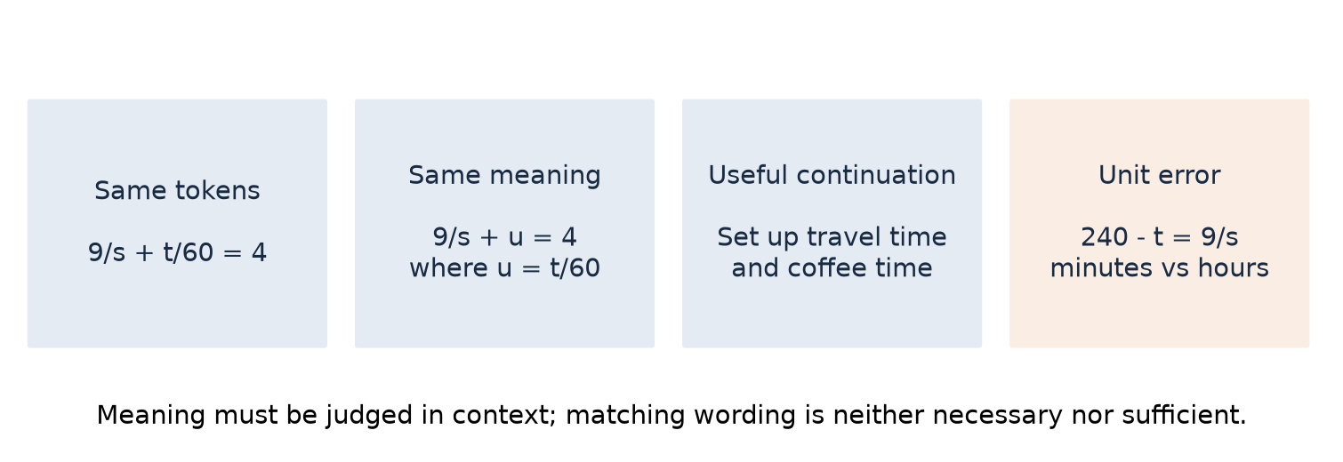
Figure 1. Teaching diagram adapted from the paper’s Figures 1-2. The first three examples illustrate different textual relationships to a valid formulation; the last contains a unit error. A high semantic-utility score is a model judgment, not a mathematical certificate.

2. Prerequisites: what exactly is being accelerated?

2.1 Sequential decoding and reasoning length

For a model producing $N$ reasoning tokens, a simple first approximation is a prefill cost plus $N$ successive decode steps. If the mean decode time is $c_B$, then the reasoning component costs roughly $Nc_B$. Real decode time depends on context length, batch size, hardware, and parallelism. Nevertheless, a long dependency chain gives a clear reason to avoid using the largest model at every position.

This matters because prefill and decode have different economics. Prefill processes a block of already-known tokens, while autoregressive decode must wait for each newly generated token before continuing. A short prefill may cost much less than generating a complete step token by token. It is not free: it still reads weights and attends to the prefix, and its advantage depends on the operating regime.

A reasoning step is also not a fixed number of tokens. It could be a sentence, a calculation, a plan, or an explicit case split. Step boundaries affect how much work is proposed before the system receives feedback. A long step amortizes a verification request but increases the amount of potentially wasted or harmful reasoning. A short step makes feedback frequent but risks turning verification itself into the bottleneck.

2.2 Token speculation and its stronger contract

In standard exact speculative sampling, let $p(x)$ be the target distribution and $q(x)$ the draft distribution at a common prefix. A sampled draft token $x$ can be accepted with probability

$$\alpha(x)=\min\!\left(1,\frac{p(x)}{q(x)}\right). \tag{2}$$

The accepted probability mass for token $x$ is then $q(x)\alpha(x)=\min(p(x),q(x))$. On rejection, sampling from the normalized positive residual $[p(x)-q(x)]_+$ restores the missing target mass. The two contributions add to $p(x)$. This is the intuition behind the distribution-preserving contract; handling the autoregressive prefix correctly extends it through a sequence.

That contract does not mean two independent random runs must emit identical text. With sampling, it means the resulting distribution matches the target distribution under the required algorithmic assumptions. Greedy variants use a different, deterministic agreement criterion. I make this distinction explicit because the paper often summarizes exact speculation as token-level equivalence, which can be read too literally.

SpecReason uses a different acceptance rule. A base-model utility score determines whether to keep an entire small-model step. There is no residual probability correction that restores the base distribution. Consequently, its appropriate quality claim is measured task accuracy under a stated budget, not lossless sampling. Exact token speculation can still operate inside a later base-model regeneration stage, but that does not make the complete outer system exact.

2.3 A score is not a probability

The paper prompts the base model for a single utility-score token, exemplified by an integer from zero to nine. A score of seven does not mean a 70% probability of correctness unless that interpretation has separately been calibrated. It is an ordinal or task-dependent judgment produced by the model. The score can reflect perceived usefulness, familiarity, local validity, or instruction following; those properties need not coincide.

This distinction becomes operational when choosing a threshold. Raising the threshold means accepting fewer candidates judged weak by that scoring setup. It does not analytically enforce a specified error rate. Nor does a maximum score imply exact token agreement. The paper’s spectrum is a helpful conceptual picture, but a semantic scoring threshold cannot by itself enforce movement toward a token-equality guarantee.

3. Method: draft, judge, and fall back

Let $h_t$ denote the question and the committed reasoning prefix before step $t$. The small model proposes $d_t$, and the base model assigns utility $u_B(h_t,d_t)$. With threshold $\tau$, a compact abstraction of the decision is

$$a_t=\mathbf{1}\{u_B(h_t,d_t)\geq\tau\},\qquad z_t=\begin{cases}d_t,&a_t=1,\\b_t\sim B(\cdot\mid h_t),&a_t=0.\end{cases} \tag{3}$$

The next prefix is $h_{t+1}=h_t\mathbin{\|}z_t$. Importantly, the fallback $b_t$ starts from the committed prefix, not from a prefix that has silently retained the rejected step. The notation abstracts away stopping tokens and task-specific output handling; it describes the paper’s step-level procedure rather than claiming a particular code interface.

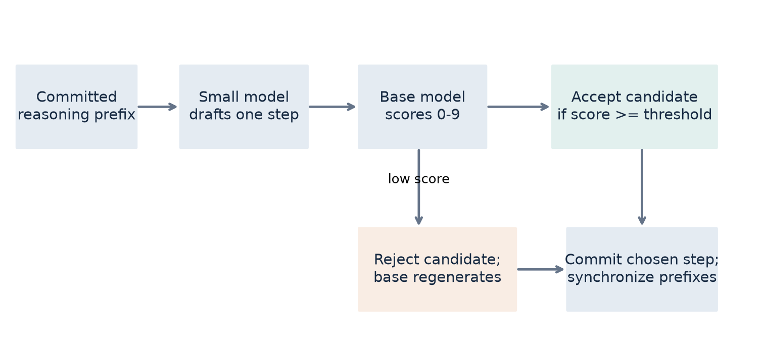
Figure 2. My schematic of Sections 4.1-4.2. The models share the logical sequence of accepted text, not hidden states or KV tensors. A rejected proposal must not remain part of the committed context.

Algorithm 1. Step-level speculative reasoning

Input: question q, small model S, base model B,
       utility threshold tau, reasoning budget K
01  h <- question q and the initial reasoning context
02  while reasoning has not terminated and budget remains:
03      remember the committed prefix h
04      d <- S generates one complete candidate reasoning step
05      u <- B scores d conditioned on the committed prefix
06      if u >= tau:
07          z <- d
08      else:
09          discard the rejected candidate's temporary state
10          z <- B regenerates a step from the committed prefix
11      append z to h and update the remaining budget
12      align each model's logical context with committed h
13  complete the answer using the chosen termination policy
Output: final answer and the committed reasoning trajectory

This pseudocode makes two bookkeeping obligations visible. First, the assessment prompt is a temporary judge view; its instructions and score must not accidentally become part of the reasoning continuation. Second, accepting text and synchronizing model state are distinct operations. A model that did not generate the accepted step still needs a consistent representation of the new prefix. These are consequences of alternating models, not extra capabilities demonstrated in the paper.

3.1 Why the base model can be a relatively cheap judge

Section 4.1 says the verification prompt reuses most of the existing chain-of-thought prefix and requires prefilling about 70 new tokens per assessment. The cost is reported as comparable to decoding one or two tokens in the studied setting. That comparison is the economic foundation of the method: the system pays for a short assessment to avoid a much longer generation.

The important phrase is “in the studied setting.” The number 70 is not a general upper bound on every candidate, context, or tokenizer. Prefix caching must actually hit, and the temporary evaluation suffix must be handled consistently. With long contexts, cache misses, a different attention architecture, or a large batch, the relation between short prefill and decode can change. It is safer to measure judge cost directly than to treat it as a universal constant.

The paper colocates the small and base models, partitions their KV-cache memory statically, and alternates execution sequentially. They do not share internal model state. The main experiments use two GPUs with tensor parallelism of two for both models; “colocation” therefore should not be misread as requiring the complete 32B model to fit on one device. The essential point is that both models occupy the same GPU resources and take turns, avoiding simultaneous kernel interference in the evaluated design.

3.2 An additional control: protect the opening plan

The paper also forces the first $n$ reasoning steps to use the base model. This protects the part of a solution where the problem is interpreted and a plan is chosen. It is a reasonable heuristic because later arithmetic may be easy only after a good decomposition exists.

However, step index is only a proxy for difficulty. A late contradiction, a difficult case split, or a tool result can require more capacity than the first few sentences. Conversely, a verbose model may spend many initial steps restating the question. I would interpret this knob as a low-cost scheduling heuristic, not a theorem that the first $n$ steps are always the important ones.

4. Deriving the latency conditions

The paper’s measurements tell us that the method can work. A small cost model helps identify when to expect it to stop working. The following equations are my analysis and assume one candidate per step, sequential execution, and an equivalent baseline step for comparison.

Let $D_t$ be draft cost, $V_t$ assessment cost, $F_t$ fallback-generation cost when rejection occurs, and $H_t$ other bookkeeping cost. Then

$$\mathbb{E}[C_t]=\mathbb{E}[D_t+V_t+H_t] +\Pr(a_t=0)\,\mathbb{E}[F_t\mid a_t=0]. \tag{4}$$

The conditioning matters. Rejected steps may be harder and longer than accepted ones. Replacing the fallback term with an unconditional average can systematically underestimate cost. Similarly, high acceptance does not imply that accepted steps save much time: they might be very short steps that the base would also produce cheaply.

For an illustrative constant-cost case, set baseline generation cost to $B$, draft cost to $D$, assessment cost to $V$, and acceptance probability to $a$. Ignore bookkeeping only for this simplified example and assume fallback costs $B$. Defining $r=D/B$ and $v=V/B$ gives

$$\frac{C}{B}=r+v+1-a,\qquad S=\frac{B}{C}=\frac{1}{r+v+1-a}. \tag{5}$$

The speedup exceeds one precisely when

$$a>r+v. \tag{6}$$

This is a useful break-even rule. A draft is not worthwhile just because it is smaller than the base. Its cost plus assessment cost must be recovered through enough accepted work. At $a=0$, the system pays for the entire failed attempt and then performs the original generation anyway. At $a=1$, the maximum speedup in this simplified model is $1/(r+v)$, so verification creates a ceiling even with perfect acceptance.

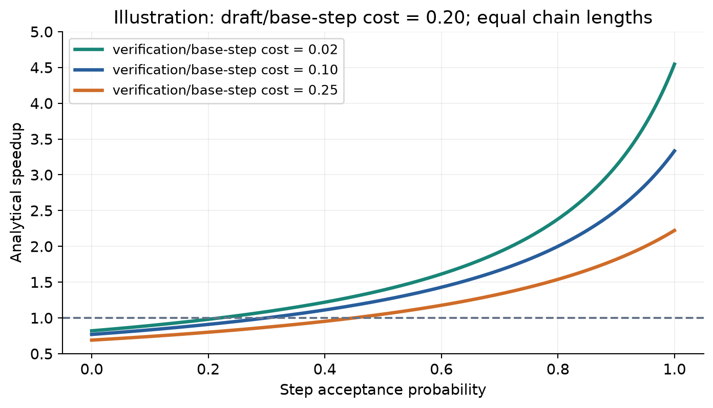
Figure 3. An illustrative calculation from Equation (5), not measured SpecReason performance. Draft cost is 0.20 of a base step; assessment cost varies. A more expensive verifier shifts the acceptance rate required for a net gain.

4.1 A concrete cost example

Suppose a base step costs 200 ms, a draft costs 40 ms, and assessment costs 10 ms. At an acceptance probability of 0.60, expected step cost is $40+10+0.40\times200=130$ ms. The speedup is about 1.54x. At acceptance 0.20, cost becomes 210 ms and the same architecture is slower than the baseline. These are hypothetical numbers chosen to expose the mechanism, not measurements from the paper.

The threshold that maximizes acceptance is therefore not necessarily the best threshold for useful service. Low thresholds may accelerate individual steps while increasing the probability of a wrong final answer or causing later backtracking. A system should optimize latency subject to an independently checked quality constraint. Optimizing the score itself would reward whatever the judge happens to approve.

4.2 Chain length changes the comparison

SpecReason also changes reasoning length, so a step-for-step comparison is incomplete. If it produces $k$ times as many roughly comparable steps as the baseline, and $f$ is the fraction of baseline latency that remains unaffected, a teaching approximation is

$$S_{\mathrm{total}}\approx \frac{1}{f+(1-f)k(r+v+1-a)}. \tag{7}$$

The approximation assumes a meaningful correspondence between average step costs. It should not be used to fit a benchmark without checking actual lengths. Its purpose is to separate two sources of speedup: using a cheaper path for a given amount of reasoning, and changing how much reasoning is generated. If $k<1$, concision helps. If the approximate trajectory causes additional reflection and $k>1$, apparent local savings can disappear.

This also explains why equal output-token budgets do not imply equal compute budgets. Assessment tokens, rejected candidate tokens, and synchronization work consume resources even when they do not appear in the final retained chain. A clear accounting should report both the final trajectory length and total work performed across models.

4.3 Step granularity is a real optimization variable

To see the trade-off, suppose a step has $m$ tokens, small-model cost per token is $c_S$, base-model cost is $c_B$, and verification has fixed cost $v_0$ plus per-token cost $v_1m$. A simplified expected cost per retained token becomes

$$\frac{C(m)}{m}=c_S+v_1+\frac{v_0}{m} +[1-a(m)]c_B. \tag{8}$$

Larger steps reduce $v_0/m$, but acceptance $a(m)$ may fall because longer proposals contain more opportunities for a consequential mistake. For the purely illustrative model $a(m)=(1-e)^m$, where $e$ is an independent per-token failure proxy, differentiating shows a balance between a negative amortization term $-v_0/m^2$ and a positive rejection term $-c_B(1-e)^m\log(1-e)$. This is not a realistic semantic-error model; reasoning errors are highly correlated. It is enough to show why neither infinitesimal steps nor arbitrarily long steps are automatically optimal.

An operational step boundary should preserve enough meaning to judge the candidate. Breaking in the middle of a variable definition can make a valid continuation look wrong; waiting until a whole paragraph is generated may hide several logical dependencies behind one score. The paper motivates complete sentences or logical units, leaving room for a more principled boundary policy.

5. Combining semantic and token speculation

The most useful compositional idea is to accelerate the fallback path as well. If the outer semantic test rejects a step, the base model regenerates it. That regeneration can use standard token-level speculative decoding. The two techniques then work at different levels: an outer decision chooses whose reasoning step to retain, and an inner mechanism accelerates generation from the chosen base model.

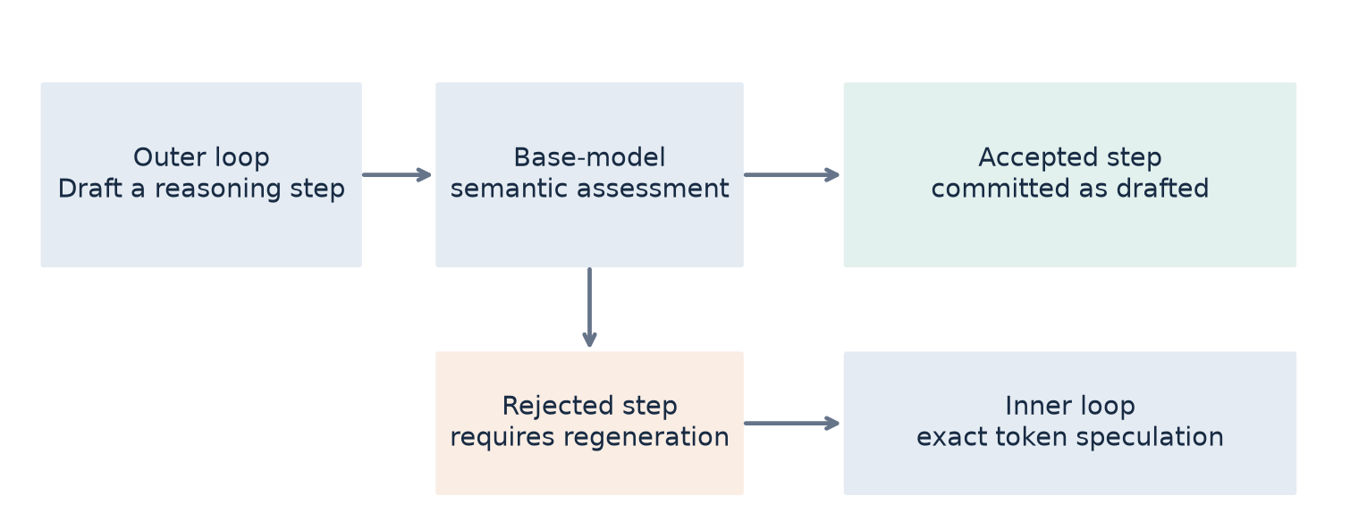
Figure 4. Teaching diagram of the paper’s hierarchical design. Token-level speculative decoding speeds up base-model regeneration after semantic rejection. It does not remove the outer draft or judge costs, and it does not restore an exact target distribution to the overall system.

Algorithm 2. Hierarchical fallback

Input: committed prefix h, candidate step d, threshold tau
01  u <- base model assesses semantic utility of d given h
02  if u >= tau:
03      commit d and return
04  restore the committed prefix before candidate d
05  initialize exact token speculation for base regeneration
06  while the replacement step has not ended:
07      draft a short token block under the current prefix
08      target model evaluates the block in parallel
09      apply the chosen exact acceptance/correction procedure
10      append only accepted or corrected target-consistent tokens
11      discard invalid speculative suffix state
12  commit the replacement step and align model prefixes

If exact token speculation speeds up fallback generation by a factor $s$, the constant-cost model becomes

$$\frac{C_{\mathrm{hier}}}{B}=r+v+\frac{1-a}{s}. \tag{9}$$

The incremental speedup over semantic speculation alone is therefore

$$\frac{C}{C_{\mathrm{hier}}} =\frac{r+v+1-a}{r+v+(1-a)/s}. \tag{10}$$

This expression is generally smaller than $s$ because only part of the outer computation is accelerated. As $a$ approaches one, there is almost no fallback left to improve. When a stricter semantic threshold increases the fallback share, exact token speculation can become more valuable. Thus the two techniques are complementary, but multiplying their standalone speedups without accounting for the remaining work is not justified.

There is also a shared-resource caveat. The same small model may serve different roles at different stages, and both models have memory footprints. A batch-serving system cannot assume that these roles consume independent spare capacity. A deployment with limited KV space may lose concurrency after adding the draft model, even while isolated-request latency improves. The paper’s sequential design establishes one operating point; a pipeline or multi-request scheduler would need its own evaluation.

6. Reading the experiments without flattening their conditions

6.1 Experimental setup and the meaning of pass@1

The main experiments combine two 32B base models, QwQ-32B and Skywork-OR1-Preview-32B, with two 1.5B models, DeepSeek-R1-Distill-Qwen-1.5B and Zyphra ZR1-1.5B. This yields four model pairs. The benchmarks are MATH500, AIME, and GPQA Diamond, spanning mathematics and graduate-level science questions. The main hardware is two NVIDIA A6000 GPUs with 48 GB each; the engine is vLLM 0.8.2 with prefix caching and tensor parallelism of two for both models.

The paper samples 16 responses per question at temperature 0.6 and averages correctness, using an 8192-token budget. This estimates single-sample success, not the probability that at least one of 16 attempts succeeds. If $c_i$ of 16 samples solve question $i$, the relevant average is

$$\widehat{\mathrm{pass@1}}=\frac{1}{M}\sum_{i=1}^{M}\frac{c_i}{16}. \tag{11}$$

A best-of-16 success metric would answer a different question and typically be much higher. Also, samples from the same problem are not 16 independent problem identities. Confidence intervals should account for this clustering. The version I read provides point comparisons but does not establish a comprehensive uncertainty analysis for every claimed small gain.

Five schemes appear in the main plot: the base model alone, the small model alone, exact speculative decoding with five draft tokens, SpecReason, and SpecReason plus token speculation. Comparing only the base and the combination would conceal how much each level contributes. The small-only baseline is equally important: it shows whether the system achieves a useful compromise beyond simply replacing the model.

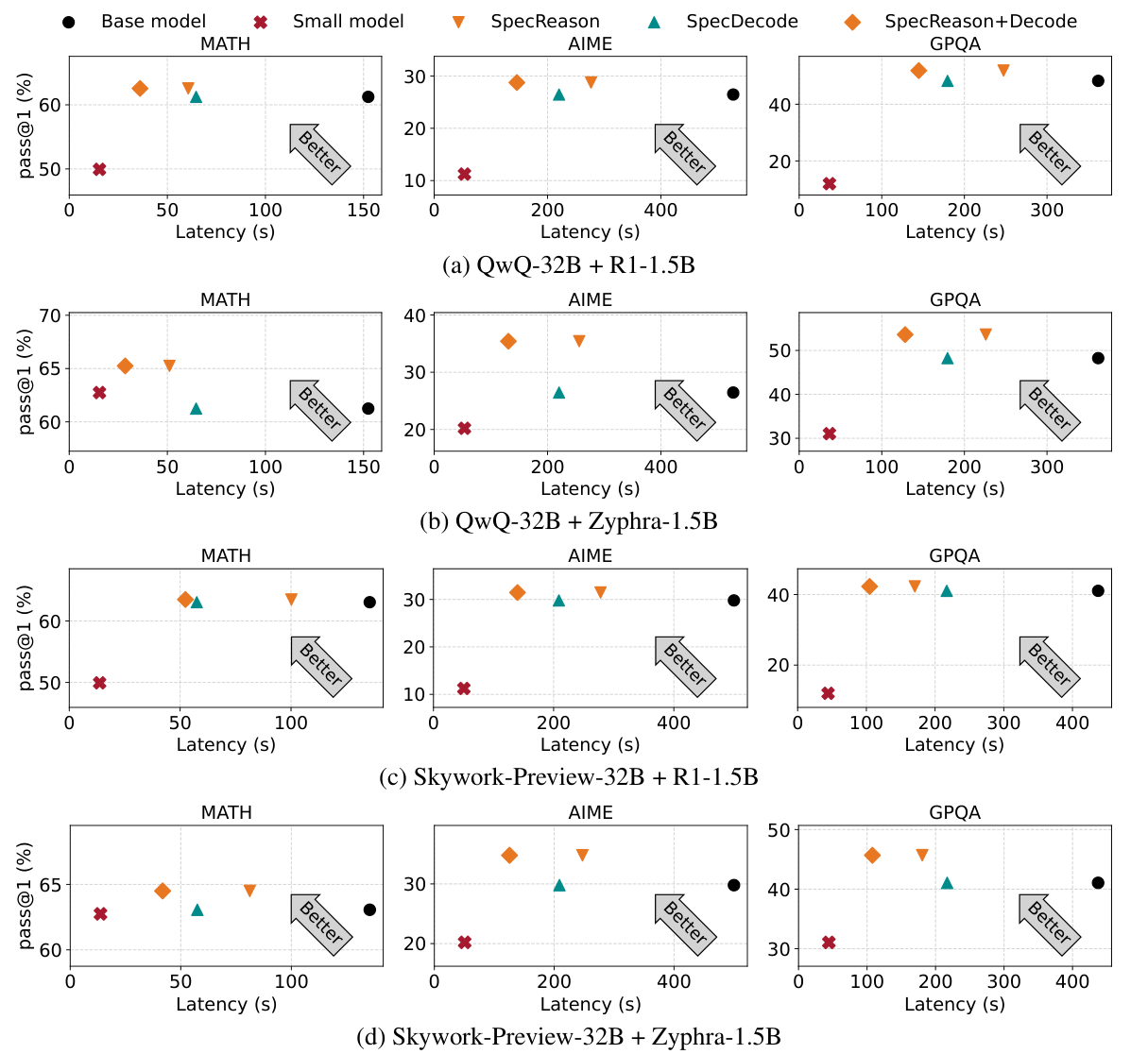
Figure 5. Original Figure 3 from SpecReason v2, page 7, cropped with its legend and all four model-pair rows. Each column is a different dataset. Upper-left is preferable within a panel. I preserve the original marks rather than infer precise values from plot pixels.

6.2 The headline ranges and what they do not mean

Section 5.2 reports the following latency-speedup ranges across the three workloads. The ranges are minima and maxima across datasets, not confidence intervals and not averages across all model combinations.

Base / small model	SpecReason versus base latency speedup	Extra latency reduction of hierarchy versus token speculation
QwQ-32B / R1-1.5B	1.5-2.5x	19.4-44.2%
QwQ-32B / ZR1-1.5B	1.6-3.0x	30.8-58.0%
Skywork-Preview-32B / R1-1.5B	1.4-2.5x	8.8-52.2%
Skywork-Preview-32B / ZR1-1.5B	1.7-2.4x	25.1-51.8%

The reported shares of steps handled by the small models are 38.1-80.0%, 36.5-71.3%, 39.3-70.2%, and 41.4-66.6% for those pairs. These are fractions of steps, not fractions of token generation time or total GPU work. A large fraction of short accepted steps can coexist with substantial fallback cost on a few difficult, long steps.

The distinction between a latency reduction and a speedup factor also matters. If a method reduces latency by fraction $\delta$, its speedup is

$$S=\frac{1}{1-\delta}. \tag{12}$$

An additional 58.0% latency reduction corresponds to about 2.38x relative to that particular comparator; 8.8% corresponds to about 1.10x. These conversions do not create new benchmark measurements. They simply prevent the mistaken interpretation that a 58% reduction means 1.58x speedup, or that two percentage reductions can be added directly.

6.3 The threshold changes quality as well as latency

The threshold sweep uses representative randomly selected subdatasets and QwQ-32B with R1-1.5B. Section 5.3 gives exact endpoint values for moving from threshold three to seven. MATH latency rises from 35.7 to 69.2 seconds and accuracy rises from 59.4% to 63.7%. AIME rises from 109.4 to 261.9 seconds and 22.3% to 39.3%. GPQA rises from 72.7 to 223.0 seconds and 33.1% to 50.7%.

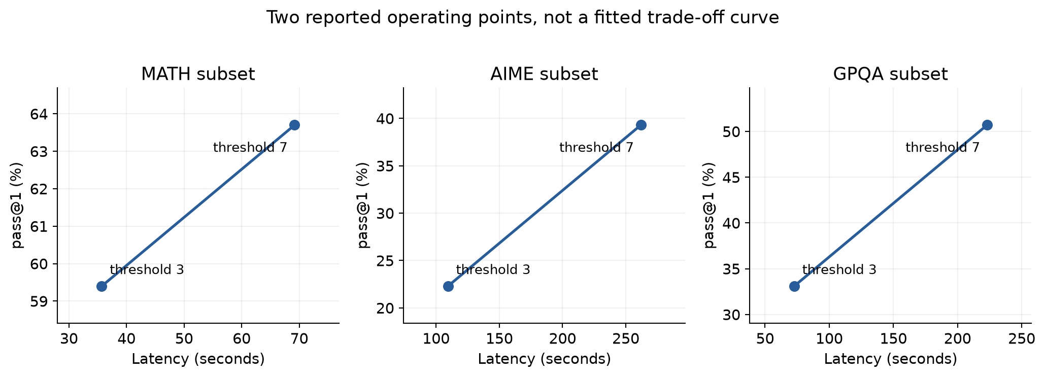
Figure 6. Redrawing of the two endpoints explicitly stated in Section 5.3. Lines connect measured endpoints only; they do not assert linear behavior between thresholds. These subdataset results should not be substituted for the full-dataset main experiment.

I find the AIME and GPQA changes particularly informative. They show why a speedup achieved by accepting almost every draft can be misleading. The small model’s capability gap is larger on those workloads, and relaxing the threshold loses accuracy much more sharply. A threshold tuned on relatively easy arithmetic therefore has no obvious right to transfer to advanced science questions.

The first-$n$-steps control offers a second operating adjustment. On the reported AIME experiment, increasing $n$ from zero through 10, 20, 30, and 40 moves accuracy from 33.2% to 37.3%, while latency moves from 270.4 to 292.6 seconds. The endpoint gain is 4.1 percentage points for 22.2 additional seconds. It is a modest, interpretable control, but these numbers do not isolate the effect of planning quality from the effect of performing more expensive-model computation.

6.4 Why a smaller model can improve a budgeted answer

The authors connect the accuracy gains partly to concision. Small models often generate shorter thinking traces, and adopting those steps can help the combined system reach a final answer before exhausting the output budget. In the QwQ-32B plus ZR1-1.5B case, the main discussion reports a 1.2-2.0x reduction in thinking-token consumption. Appendix A.2 reports pair-specific ranges of 1.0-1.3x, 1.2-2.0x, 1.0-1.8x, and 1.1-2.3x.

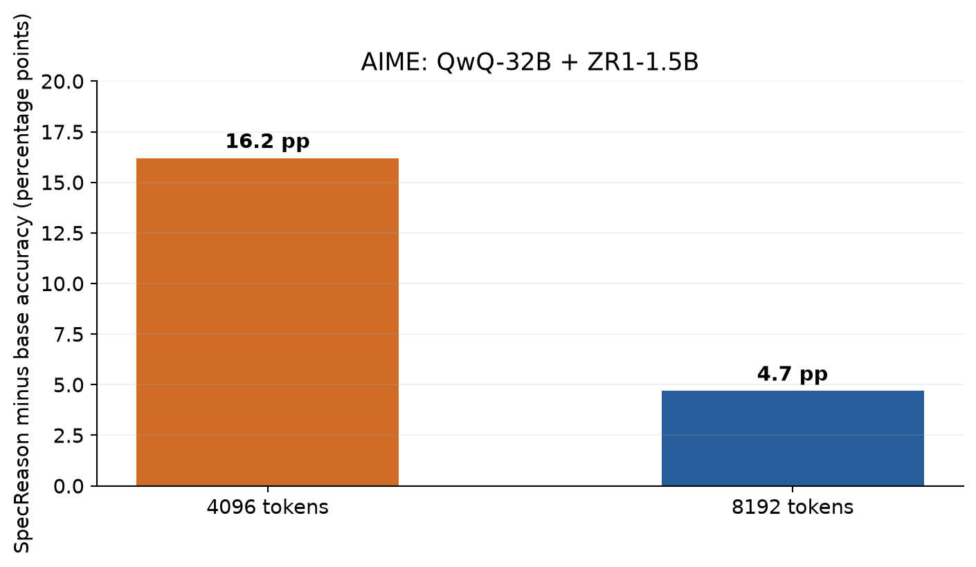
Figure 7. Reported AIME accuracy gaps for QwQ-32B plus ZR1-1.5B: 16.2 percentage points at 4096 tokens and 4.7 points at 8192 tokens, from the Section 5.2 discussion of Figure 4. These are differences on the accuracy scale, not multiplicative improvements.

This supports a budget-aware interpretation: the hybrid policy may use an imposed output allowance more effectively. It does not by itself prove that the small model contributes a superior reasoning algorithm. Explicit judgment, shorter traces, a changed path distribution, and better termination behavior can all contribute. An equally concise base-model control would help separate those explanations.

The budget effect is also a warning about causal language. A plot of fewer tokens alongside better accuracy establishes an association under the method, not a complete mediation analysis. The paper plausibly attributes part of the gain to less verbosity and part to structured assessment. The evidence is consistent with those explanations, but does not quantify each mechanism’s independent contribution.

6.5 What the judge comparison establishes

The paper compares the base model’s utility judgments with Math-Shepherd process-reward scores on small-model AIME steps. It groups the PRM scores into bins and plots the average base-model utility in each bin. Lower PRM scores generally align with lower utility scores, and the curve rises before flattening. This is useful evidence that the base model is not assigning entirely arbitrary numbers.

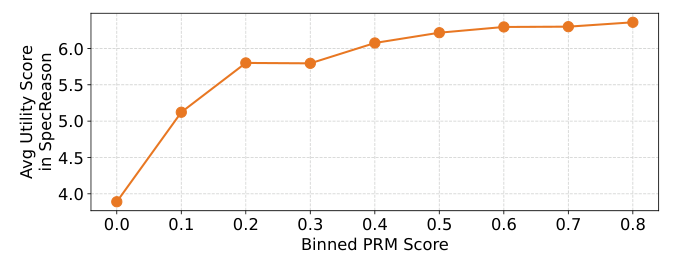
Figure 8. Original Figure 7 from SpecReason v2, page 9. The horizontal axis bins a separate PRM’s score; the vertical axis averages the base-model utility score. Binned association does not provide step-level calibration, false-acceptance rates, or a guarantee of final-answer correctness.

There are several limits to that evidence. The PRM is another learned judge, rather than ground truth. A bin average can hide a mixture of very good and very bad judgments. The plot does not show the number of observations or dispersion in each bin. Finally, both judges may miss the same systematic error, such as a globally inconsistent assumption that looks locally fluent. I treat the figure as support for discriminative usefulness, not proof of verification reliability.

6.6 Portability: a larger base model is not automatically a better setting

Appendix A.1 replaces the 32B base with R1-70B on four A100-80GB GPUs using tensor parallelism of four. On the representative AIME subdataset, the reported speedup is 1.5x, below the 1.9x QwQ-32B comparison. The base model’s time per token improves by about 1.5x on the stronger hardware, while the small model improves by only about 1.1x. The relative cost advantage of drafting narrows.

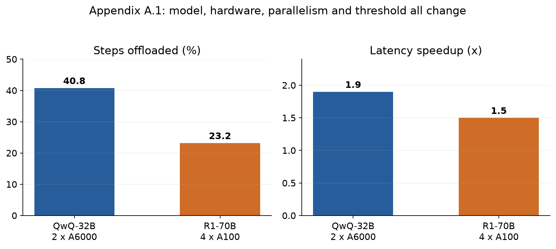
Figure 9. Redrawing of Appendix A.1’s reported offloading shares and speedups. Model family, hardware, parallelism, and acceptance threshold change together. This comparison is evidence of hardware and model dependence, not an isolated experiment on parameter count.

The appendix also uses a stricter threshold for R1-70B to preserve quality, reducing the offloaded step share from 40.8% to 23.2%. Two effects therefore work in the same direction: the baseline gets relatively faster, and less work is delegated. This is exactly the kind of situation captured by the break-even model. The number of parameters alone is a poor predictor of the resulting speedup.

7. Design alternatives and failure boundaries

7.1 A separate PRM versus the base model as judge

A dedicated process reward model can make verification more specialized, potentially smaller, and easier to calibrate for a narrow domain. Its disadvantages include another resident model, another context representation, and possible domain shift. The base-model judge reuses a model already present for fallback and can exploit its understanding of the task. Its weakness is that good generation ability does not guarantee robust critique or score instruction following.

The paper’s choice is sensible as a minimal system, particularly when a short cached assessment is cheap. It should not be generalized into a claim that a generic base model always dominates a trained PRM. The relevant comparison includes latency, memory, failure correlation, and final-answer accuracy at matched budgets.

7.2 Routing before drafting versus judging afterward

A pre-step router could choose the small or large model without paying for a rejected draft. That seems cheaper, but predicting the difficulty of a step before seeing its content is harder than assessing a concrete proposal. SpecReason pays the draft cost to obtain evidence for its decision. The cost model makes this price explicit.

A hybrid policy could route obvious hard transitions directly to the base model and use proposal-and-judge on uncertain or routine work. Such a policy is a plausible extension, not an evaluated feature of this version. It would need a comparison against the existing threshold system with routing overhead included.

7.3 Why local validity is not enough

An intermediate statement can be mathematically true yet strategically useless. It can also be locally consistent with a mistaken earlier premise. Accepting it may consume the budget without moving toward an answer, or reinforce an error that should have triggered a change of plan. A utility judge ideally needs to assess contribution to downstream success, which is harder than checking grammar or one calculation.

Self-reflection may repair some accepted mistakes, but it is not a free recovery mechanism. Repairs cost tokens, can arrive too late, and are themselves fallible. This matters when a relaxed threshold appears to preserve average accuracy: the same average can hide a different distribution of failures, longer tails, or more severe errors on a subset of tasks.

7.4 A simple risk bound clarifies the missing measurement

Let $E_t$ be the event that a harmful candidate is accepted at step $t$, and let $u_t=\Pr(E_t)$. Without assuming independence, the union bound gives

$$\Pr\!\left(\bigcup_{t=1}^{n}E_t\right)\leq\sum_{t=1}^{n}u_t. \tag{13}$$

This is a bound on at least one harmful accepted step, not on final-answer error. Recovery can make the final answer correct despite such an event; base-model mistakes can make an answer wrong even with no such event. Still, it shows why a low-looking per-step error rate can become consequential over a long trajectory. To use the bound operationally, one would need actual harmful-acceptance estimates, not raw ordinal scores.

If $q_t$ is the probability that a draft is harmful and $\beta_t$ the probability that the judge accepts it conditional on that harm, then

$$u_t=q_t\beta_t. \tag{14}$$

This decomposition separates draft quality from verifier behavior. Improving either can help, but the two may be correlated through shared training or blind spots. It also shows why overall acceptance rate alone is insufficient: a system can accept many safe routine steps while still letting through the few mistakes that determine the answer.

8. Limitations of the evidence

The strongest supported conclusion is that the tested models and workloads contain enough cheap, useful intermediate steps for a base-model judge to deliver a favorable accuracy-latency trade-off. The evidence is narrower than a universal reasoning accelerator. Most experiments involve mathematical or science question answering, and the main pairs share the Qwen lineage. The 70B appendix broadens the evidence, but also changes hardware and parallelism.

The threshold sweeps use subdatasets. A configuration chosen after looking at benchmark outcomes risks overstating how well the same threshold will generalize. A held-out calibration set, a separately locked test set, and confidence intervals for quality differences would make the operating-point claim stronger. In particular, the smallest reported accuracy changes deserve uncertainty estimates rather than categorical interpretations.

The paper does not establish a comprehensive throughput, tail-latency, or energy result for a saturated multi-tenant server. Sequential alternation simplifies interference, but introduces switching and memory-partition consequences. The headline speedup should not be silently repurposed as a claim about GPU cost per thousand user requests under arbitrary load.

Finally, a single-token judge can be brittle to candidate length, style, task language, or instructions embedded in the candidate text. The paper does not provide a full adversarial robustness study of that interface. For benign numerical benchmarks this may not dominate; in agentic settings with untrusted external text, the semantic boundary would need additional scrutiny. This is a boundary of applicability, not a claim that the reported experiments used hostile inputs.

9. Critical analysis

9.1 The real contribution is a changed optimization objective

I find SpecReason compelling because it asks what must be preserved. If users care about the final answer under a latency budget, preserving every internal token is often more restrictive than necessary. The paper makes that freedom operational with a concrete small-model proposal and a cheap large-model judgment. This is a substantive change in the inference policy, not merely a faster implementation of the original sampler.

The trade-off is that correctness becomes an empirical property of a composed system. Exact sampling provides a clean contract independent of a particular benchmark’s answer metric. Semantic acceptance offers more freedom but must earn its quality claim on each relevant task distribution. Both contracts are useful, and conflating them would make deployment decisions worse.

9.2 A high score should be tested against outcomes it did not define

The judge controls which trajectories survive. If evaluation also uses the same judge’s preference, the system can appear to improve by becoming more judge-friendly. The paper’s final-answer benchmarks reduce this problem because answer correctness is evaluated separately from the step utility score. The binned PRM agreement is supplementary evidence, not the core quality target.

For future work, I would preserve that separation. Calibrate a threshold on one set of problems, then report final success and harmful-acceptance behavior on independent problems. Analyze cases where both judges agree but the final answer is wrong. Those cases reveal shared blind spots that a correlation plot cannot expose.

9.3 The most informative next comparison is matched compute

At a fixed output-token budget, shorter drafts may improve completion rates. That is a valuable practical result. To understand the mechanism more deeply, I would compare systems at matched wall-clock time and matched total GPU work, while retaining the fixed-token-budget result as a separate view. The relevant work includes discarded proposals and judging, not only the accepted reasoning trace.

A suitable decision objective is a latency minimization constrained by independently measured final quality:

$$\min_{\tau,n,\mathcal{G}}\;\mathbb{E}[T] \quad\text{subject to}\quad \mathrm{Accuracy}(\tau,n,\mathcal{G})\geq A_{\min}, \tag{15}$$

where $\mathcal{G}$ denotes a step-boundary policy. This is my formulation, not an optimization solved by the paper. It makes clear that threshold, protected-prefix length, and granularity interact. It also encourages reporting a family of operating points rather than selecting a single favorable headline after seeing the test results.

9.4 What would change my assessment

I would gain confidence from a study that isolates four mechanisms: drafting with a smaller model, shortening the base model’s own trace, adding explicit judgments, and changing fallback generation. A matched-budget comparison with a concise base-model control would show whether semantic delegation adds value beyond brevity. A separate judge ablation would show whether generation capability or calibration matters more.

I would become more cautious if accuracy gains vanished when truncation was removed, if harmful-acceptance rates rose sharply with context length, or if the draft model’s memory footprint erased throughput gains under load. None of these outcomes is established here. They are discriminating tests suggested by the paper’s design and current evidence.

The broader research direction is attractive: treat intermediate reasoning as structured work that can be scheduled across models, while keeping verification cost and error propagation visible. SpecReason provides an accessible first system for that idea. Its enduring lesson is to optimize useful reasoning progress per unit of total work, with a quality contract that is stated honestly.

10. Conclusion

SpecReason delegates individual reasoning steps to a small model and uses the large model for inexpensive assessment and selective fallback. Its measured gains depend on meaningful step boundaries, low assessment cost, adequate acceptance quality, and a real speed gap between the models. Token-level speculative decoding can further accelerate the fallback branch, but only that branch’s share of the work.

My practical reading is to begin with the cost inequality, then inspect the final-answer evidence under the actual budget. A fast local draft is useful only if acceptance and subsequent reasoning recover its cost without unacceptable errors. The paper demonstrates that this can happen; it also makes clear why threshold calibration, workload transfer, and honest compute accounting are the next important questions.

References and figure notes

1. Rui Pan, Yinwei Dai, Zhihao Zhang, Gabriele Oliaro, Zhihao Jia, Ravi Netravali. SpecReason, arXiv:2504.07891v2, 2025-05-16. Primary source for all reported measurements, Sections 4-5 and Appendix A.
2. Yaniv Leviathan, Matan Kalman, Yossi Matias. Fast Inference from Transformers via Speculative Decoding, 2023. Background for the exact speculative-sampling contract.
3. Peiyi Wang et al. Math-Shepherd: Verify and Reinforce LLMs Step-by-step without Human Annotations. The PRM used in SpecReason’s judgment comparison; the comparison itself is reported in SpecReason Section 5.4.

Figures 5 and 8 reproduce cropped plots from the primary paper with attribution. Figures 6, 7, and 9 redraw values explicitly stated in its prose. Other figures are explanatory constructions. Equations (2) and its probability-mass explanation describe the standard background algorithm; Equations (4)-(10) and (13)-(15) are this review’s conditional models or analysis. They should not be mistaken for new benchmark results or guarantees claimed by SpecReason.