EvoRubric: Who Teaches a Model to Write Its Own Grading Criteria?

Review date: October 20, 2026
Author: Zhongzhu Zhou
Paper reviewed: EvoRubric: Self-Evolving Rubric-Driven RL for Open-Ended Generation
Paper authors: Xin Guan, Xiaomeng Hu, Shen Huang, Zhenyi Wang, Bo Zhang, Zijian Li, Pengjun Xie, Bo Liu, Jiuxin Cao
Paper: arXiv:2605.29847v2, revised October 8, 2026

1. The question behind the method

When a model writes an answer to an open-ended question, a single reference answer is often an inadequate teacher. A useful answer can be concise or expansive, organize evidence in different orders, and make different but defensible choices about emphasis. Yet reinforcement learning still needs a numerical signal. Rubrics provide one bridge: replace an opaque overall impression with a collection of explicit conditions, apply those conditions to the answer, and aggregate their scores.

The difficult part is deciding which conditions should exist. A fixed checklist can become easy to satisfy while missing newly emerging failure modes. An external model can keep inventing new criteria, but it is not necessarily learning which criteria actually improve the policy being trained. EvoRubric makes criterion construction a trained behavior of the same policy that produces answers. Its central question is how to reward that behavior when final-answer correctness cannot provide an unquestionable reference.

My reading is that the contribution is a particular decomposition of supervision. Validity, discrimination, and agreement are treated as different signals. A criterion should be defensible, distinguish some current answers, and participate in a scoring pattern supported by other rubric samples. These properties are complementary; none alone establishes that the final answer is correct.

This distinction matters because the framework retains fixed external anchors. The answer-producing policy and rubric-producing policy share trainable parameters, but the Meta-Verifier is a frozen copy of the initial policy. A separate frozen Grader applies criteria to answers. The system discovers new descriptions of quality inside boundaries partly supplied by those frozen models. It does not create an independent source of truth.

Figure 1 (paper Fig. 1). The paper distinguishes expert-written, model-written static, externally evolving, and shared-policy evolving rubrics. The meaningful difference is which criterion-generation behavior receives training feedback.

1.1 What this review covers

I read the complete 22-page v2, including Appendices A-J. The equations below restate its reward construction and add explicitly identified derivations and toy examples. Replotted benchmark and audit figures use the paper’s reported numbers. I have not trained these models or independently reproduced their benchmark scores.

EvoRubric, singular, is arXiv 2605.29847. It should not be confused with the separately authored EvoRubrics paper, arXiv 2606.23038. Similar names do not imply a shared method or interchangeable resources.

2. Prerequisites: from text to a learning signal

2.1 A criterion is a conditional scoring rule

Consider a non-medical explanatory task: explain a result and identify supporting evidence. A positive criterion might reward covering the main result. A negative criterion might penalize inventing a supporting claim. The grader decides whether the condition occurs; the sign of the criterion’s weight determines whether occurrence is good or bad.

Let $w_c$ be the signed weight of criterion $c$, and let $z_c(o)\in\{0,1\}$ indicate whether output $o$ exhibits that criterion. For a negative criterion, $z_c(o)=1$ means the undesirable behavior actually occurs. It does not mean the answer successfully avoids that behavior. Keeping this convention straight is essential when reasoning about filtering and saturation.

The raw score and total positive and negative weight masses are

$$A(o;C)=\sum_{c\in C}w_cz_c(o),\qquad P(C)=\sum_{c\in C}\max(w_c,0),\qquad N(C)=\sum_{c\in C}\max(-w_c,0). \tag{1}$$

These are sums over the entire criterion set. The denominator used below is shared across answers, rather than being recomputed using only criteria an answer happens to satisfy. A response therefore cannot improve its normalized score merely by causing a difficult criterion to vanish from its own denominator.

2.2 Why the normalization stays bounded

Appendix C normalizes the signed sum by the larger weight mass:

$$F(o;C)= \begin{cases} A(o;C)/\max\{P(C),N(C)\},&\max\{P(C),N(C)\}>0,\\ 0,&\text{otherwise}. \end{cases} \tag{2}$$

To see the bound, split the raw sum into its positive and negative parts. Binary indicators imply that the positive contribution lies between zero and $P$, and the negative contribution lies between $-N$ and zero. Consequently $-N\leq A\leq P$. Dividing by a number at least as large as either mass yields $-1\leq F\leq1$.

The bound does not imply a symmetric attainable range. If all criteria are positive, possible scores lie in $[0,1]$. If they are all negative, they lie in $[-1,0]$. A zero score in the latter case can mean that no penalized behavior occurred. Empty sets and sets with only zero weights also receive zero, but for an entirely different reason: they supply no scoring information.

In the constructed example in Figure 2, the weights are $+4,+2,-3$, so $P=6$, $N=3$, and the common denominator is 6. Answer A satisfies both positive conditions and avoids the error, obtaining 1. Answer C satisfies both positive conditions but commits the error, obtaining 0.5. Answer D earns no positive points and commits the error, obtaining -0.5. These are illustrative calculations, not outputs sampled from a model.

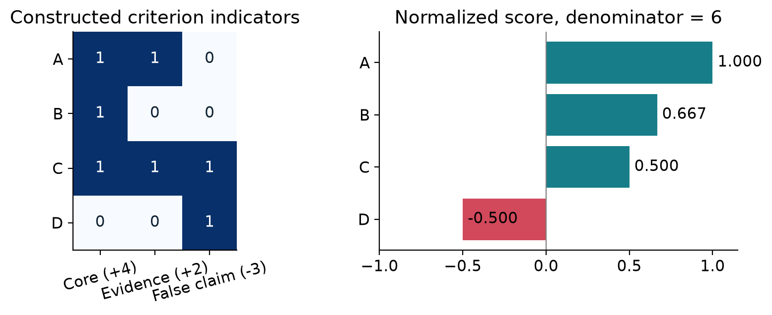
Figure 2. Original toy calculation of Appendix C’s normalization. A negative criterion is activated by the error itself. All four answers share the same denominator.

2.3 Group-relative learning needs differences

GRPO compares multiple samples for the same input. EvoRubric computes advantages separately for each query and each role:

$$\widehat A_i=\frac{r_i-\mu}{\sigma+\varepsilon}. \tag{3}$$

If all eight answers receive the same reward, the numerator is zero for every answer. The numerical stabilizer avoids division by zero but cannot manufacture a useful direction. This explains why discrimination matters. A criterion can be perfectly valid yet give no relative learning signal for the current group.

For example, rewards $[1,0.5,0.5,0]$ have mean 0.5. Ignoring a negligible stabilizer and using population standard deviation, the advantages are approximately $[1.414,0,0,-1.414]$. The update favors the first sample relative to the fourth. The two middle samples carry no direct advantage in this group, although they still affect the group’s statistics.

Validity and usefulness are therefore distinct. A requirement that every answer already meets may be worth retaining for evaluation or regression prevention, but it does not help this particular group-relative update. EvoRubric treats that distinction differently in its fixed base rubric and its changing memory.

3. Four roles, two trainable behaviors

The architecture is easier to follow if the word “judge” is avoided until the roles are separated.

Role	Parameters during RL	Main responsibility
Reasoner	Shared trainable policy	Produce answers
Rubric Generator	Same trainable policy	Propose missing criteria
Meta-Verifier	Frozen initial policy	Screen criterion validity
Grader	Frozen GPT-OSS-120B	Apply retained criteria to answers

The policy uses Qwen3-8B or Qwen3-14B. Role-specific prompts determine whether it generates an answer or a rubric. Sharing parameters makes improvements transferable between the two behaviors, but also makes them interfere. A change learned from answer generation can alter rubric generation even when no explicit Generator loss is applied.

For each query, the Reasoner first generates eight responses. The Generator sees the query, sampled responses within its input budget, fixed base criteria, and historical criteria. It produces four candidate rubric sets. This ordering is important: the candidates are grounded in differences among actual current responses, rather than being generic lists invented before observing the policy.

Each query has its own memory, capped at ten evolved criteria. The base criteria are stored separately and remain fixed. Appendix D reports between two and eight base criteria per prompt, with six being the most common count. Memory is thus an extension of a persistent anchor, not a replacement for that anchor.

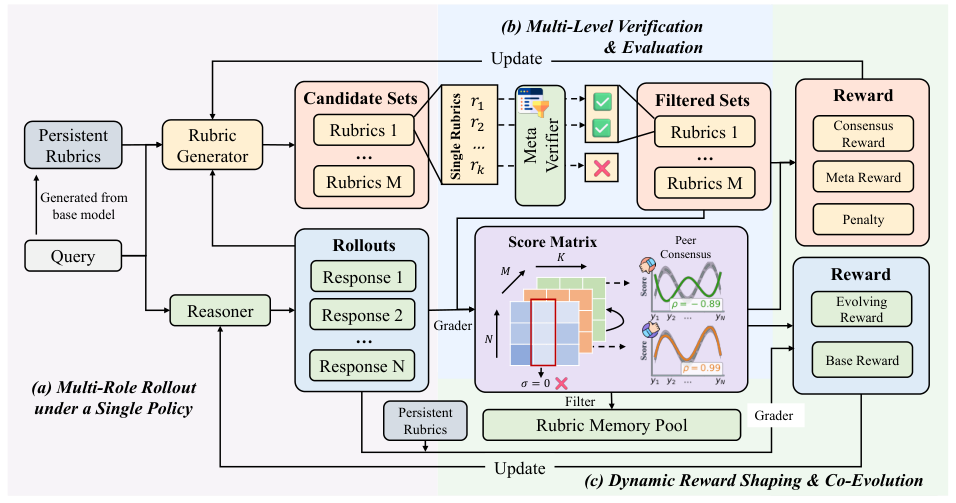
Figure 3 (paper Fig. 2). Response sampling precedes criterion discovery. Validity checks and criterion grading generate role-specific rewards; selected criteria persist into the next visit to the query.

3.1 Why freeze the validity check?

A moving validity checker and a moving criterion generator could reinforce each other’s mistakes. Freezing the initial policy gives the generator a relatively stable acceptance boundary. Freezing the Grader likewise avoids changing the rule-execution mechanism at the same time as the rules.

The tradeoff is that a frozen initial model may misunderstand a sophisticated but valid criterion discovered later. It can also consistently accept a familiar false criterion. Stability makes drift easier to interpret; it does not guarantee correctness or unlimited headroom.

The method still relies on a much larger training Grader, GPT-OSS-120B. The statement that criterion learning happens inside an 8B policy should therefore not be interpreted as a complete 8B-only training stack. The learned component and the total supervisory resources are different quantities.

3.2 What the prompts actually encourage

Appendix J asks the Generator to identify observable differences missing from existing criteria, prefer sparse nonredundant rules, and return an empty list when there is no meaningful gap. Positive rules describe desirable properties; negative rules describe active errors. That last choice makes the sign convention in Equation 1 operational.

The Meta-Verifier uses domain-specific screening categories. In Medical, these include factual conflict, unmeasurable conditions, duplication, generic criteria, and unsupported length or style requirements. In Writing and Science, explicit task constraints and factuality also matter. These checks define an intended boundary around learned criteria, but their reliability must be evaluated rather than inferred from the strength of the prompt wording.

4. Learning to propose useful criteria

4.1 Validity is measured before filtering

Suppose a candidate batch proposes $K_m$ criteria and $V_m$ pass verification. The validity reward is

$$a_m=\frac{V_m}{\max(1,K_m)}. \tag{4}$$

The denominator includes rejected proposals. Otherwise a batch that proposes ten invalid rules and one acceptable rule could appear as valid as a batch that proposes only the acceptable rule. An empty batch receives zero validity reward.

Let $D_m$ count verified criteria whose score vectors across the answers are nonconstant. Combining the description in Appendix C gives the discriminative contribution

$$d_m=a_m\frac{D_m}{\max(1,V_m)}. \tag{5}$$

For $V_m>0$, this simplifies to $D_m/K_m$. Thus invalid proposals dilute the reward even when the surviving rules separate responses well. This simplification is my algebraic restatement of the paper’s “verified fraction scaled by validity fraction,” not an additional training mechanism.

The filter asks whether standard deviation is strictly positive, not whether the variance exceeds a robustness margin. With binary criterion judgments, one exceptional response can make a rule discriminative. That is useful for discovering rare errors, but also makes the signal vulnerable to a single mistaken grading decision.

4.2 Peer consensus evaluates score patterns

For each verified batch, construct a vector of normalized scores across the same $N$ answers:

$$\mathbf v_m= \big[F(o_1;\widetilde R_m),\ldots,F(o_N;\widetilde R_m)\big]^\top. \tag{6}$$

The peers used for batch $m$ are the other batches with nonconstant score vectors. Their average and the resulting Pearson correlation are

$$\overline{\mathbf v}_{-m} =\frac{1}{|\mathcal P_m|}\sum_{j\in\mathcal P_m}\mathbf v_j, \qquad \rho_m=\operatorname{corr} (\mathbf v_m,\overline{\mathbf v}_{-m}). \tag{7}$$

Pearson correlation compares centered scoring patterns. Multiplying one vector by a positive constant or adding a constant offset does not change its correlation with another vector. It therefore rewards agreement about relative variation across answers, rather than agreement about absolute score levels.

When there is no nonconstant peer, or the mean peer vector is constant, consensus is set to zero. Two individually nonconstant peers can cancel when averaged, so checking individual variances is insufficient. A verified candidate batch becomes eligible for current supervision and memory selection only when its own score vector is nonconstant and its LOO correlation is greater than 0.2.

The contribution to Generator reward is the positive correlation scaled by validity:

$$\widetilde\rho_m=a_m\max(0,\rho_m). \tag{8}$$

Eligibility and reward contribution should not be collapsed into a single concept. The paper describes a threshold for which batches contribute to the Reasoner’s current rubric supervision. It separately describes positive consensus as part of the Generator reward, alongside validity and discrimination.

4.3 Why exclude the batch itself?

If a vector contributes to the reference against which it is compared, agreement can be inflated mechanically. Figure 4 uses centered vectors $u=(-1,-1,1,1)$ and $v=(-1,1,-1,1)$. They are orthogonal, so their correlation is zero. Yet the correlation between $u$ and $(u+v)/2$ is $1/\sqrt{2}$, approximately 0.707.

An even sharper example compares $u$ with $-u/2$. True peer correlation is -1. Including $u$ in the average gives $u/4$, which correlates perfectly with $u$. Leave-one-out removes this self-contribution. It does not remove common errors shared by different samples of the same model.

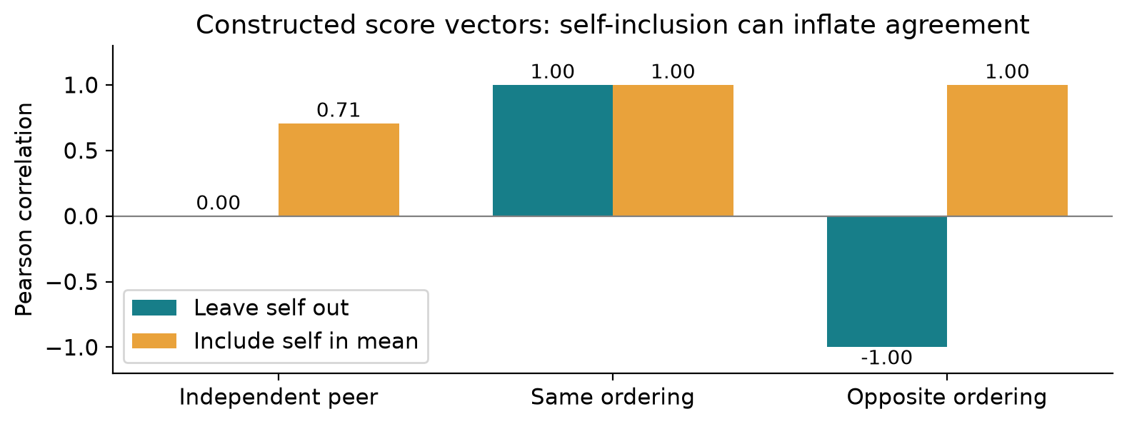
Figure 4. Original constructed examples showing self-inclusion bias. These correlations are algebraic illustrations, not estimates of the paper’s observed training behavior.

4.4 Why consensus is not a correctness test

All four rubric sets are sampled from the same current policy, see related input, and are evaluated by the same Grader. Their errors need not be independent. A shared preference for a particular style can create high agreement even when that style is irrelevant. A novel, valid minority criterion can disagree with the majority and fail the eligibility threshold.

The Meta-Verifier is intended to reduce this problem by checking criterion meaning before scores enter consensus. The fixed base rubric supplies another anchor. The empirical question becomes whether those anchors are strong enough to prevent peer agreement from amplifying plausible mistakes. The human audit later in the paper is directly relevant to that question.

5. Rewards, memory, and the joint update

5.1 The Generator has more regularization than the headline equation

The main text combines consensus, validity, and discrimination with count and length penalties. Appendix C adds a point-concentration penalty. For a well-formed rubric output, the complete description is therefore

$$R_{\mathrm{gen},m} =\widetilde\rho_m+a_m+d_m -p_{\mathrm{num}}-p_{\mathrm{len}}-p_{\mathrm{conc}}. \tag{9}$$

The count penalty is zero up to ten proposed criteria and then rises linearly to a cap of one:

$$p_{\mathrm{num}} =\min\!\left(1,\max\!\left(0,\frac{K-10}{10}\right)\right). \tag{10}$$

For at least three criteria, let $f$ be the fraction sharing the most frequent absolute weight. The point-concentration penalty is $0.5\max(0,(f-0.6)/0.4)$; it is zero for fewer than three criteria. This discourages assigning the same magnitude to almost every criterion. It is a heuristic about weight diversity, not a proof that varied weights reflect better calibrated importance.

Both roles receive an overlong-output penalty. With the reported settings,

$$p_{\mathrm{len}}(y) =\max\!\left(0,\frac{\ell(y)-4096}{4096}\right). \tag{11}$$

The penalty is zero at 4096 tokens, 0.5 at 6144, and 1 at 8192. It depends on token length, not characters or words. A model may consequently learn brevity partly because of this explicit shaping, rather than because its criteria alone discover that shorter answers are better. Malformed Generator outputs receive a format reward of -2; empty or fully rejected batches add no criteria.

5.2 Current evidence and persistent memory are different

Let $H$ contain historical criteria that distinguish the current response group, and let $\mathcal E$ index eligible current batches. Then

$$S_{\mathrm{current}}(o)= \begin{cases} \frac{1}{|\mathcal E|}\sum_{m\in\mathcal E}F(o;\widetilde R_m), &|\mathcal E|>0,\\ 0,&|\mathcal E|=0. \end{cases} \tag{12}$$

The pool contribution and final Reasoner reward are

$$S_{\mathrm{pool}}(o)=\tfrac12F(o;H)+\tfrac12S_{\mathrm{current}}(o), \qquad R_{\mathrm{rea}}(o)=F(o;C_{\mathrm{base}})+S_{\mathrm{pool}}(o)-p_{\mathrm{len}}(o). \tag{13}$$

The coefficients remain one half when one source is absent. On the first visit to a query, historical memory is empty, so the current batches contribute at half strength. The remaining half is not reassigned to current feedback. Likewise, if no current batch qualifies, historical supervision stays at half strength.

As an illustrative calculation, a response with base score 0.6, historical score 0.2, current score 0.8, and no length penalty receives $0.6+0.1+0.4=1.1$. On a first visit with the same base and current scores, its reward is 1.0. If only historical feedback is available, it is 0.7. These examples show why memory availability changes the effective scale of supervision.

Current supervision averages every eligible batch. Persistent memory, however, accepts new criteria only from the eligible batch with the highest LOO consensus. Confusing those two paths would change both the immediate reward and the future curriculum.

5.3 Zero variance is not always mastery

A historical positive criterion is saturated when all responses satisfy it. A negative criterion is saturated when all responses avoid the penalized behavior. Those entries can be retired from memory.

An equally important opposite case is unanimous failure: all responses miss a positive requirement, or all commit a negative error. Such a criterion also has zero variance, and therefore does not enter the historical score for the current group. But it is not saturated in the desired-behavior sense. The paper’s distinction permits it to remain in memory rather than treating collective failure as success.

This is a boundary of relative learning. A group of uniformly poor answers provides no internal contrast on that dimension. The fixed base score and other variable criteria may still drive learning, but the hard dimension itself offers no direct ordering until some sampled answer behaves differently.

Memory insertion checks exact textual duplication against retained entries. The validity checker also considers semantic overlap with base criteria. Neither fact means that the persistent pool is perfectly semantically deduplicated. The human audit explicitly measures a stronger notion of distinctness.

Algorithm 1. One query’s scoring and memory transition

01  Read fixed base criteria B and snapshot historical memory H_old.
02  Sample N = 8 answers using the rollout policy.
03  Sample M = 4 rubric sets conditioned on answers, B, H_old.
04  Screen each proposed criterion with the frozen Meta-Verifier.
05  Grade answers against B, H_old, and verified new criteria.
06  Form batch score vectors; compute validity and discrimination.
07  Compute LOO correlations using other nonconstant batch vectors.
08  Identify eligible new batches: nonconstant vector and rho > 0.2.
09  Compute Generator and Reasoner rewards from this snapshot.
10  Remove truly saturated historical entries from persistent memory.
11  If any batch is eligible, choose the highest-consensus batch.
12  Add its criteria after duplicate checks against retained memory.
13  Evict oldest entries until the per-query pool has at most 10.
14  Keep fixed base criteria unchanged for all future visits.

The snapshot at line 1 matters. Newly admitted memory is for a later visit, while current criteria already contribute through Equation 12. Updating memory before scoring without preserving the historical snapshot could count the same discovery through both paths.

5.4 Shared parameters do not imply shared advantage statistics

For each query, the eight Reasoner samples form one advantage group and the four Generator samples form another. Their rewards have different meanings and scales, so they are standardized separately. The combined batch then updates the shared policy with a token-averaged clipped objective.

Writing $r_{b,t}(\theta)$ for the token likelihood ratio to the rollout policy, Appendix B specifies

$$J(\theta)=\mathbb E\!\left[ \frac{\sum_{b\in\mathcal B}\sum_{t=1}^{|y_b|} \min\{r_{b,t}\widehat A_b, \operatorname{clip}(r_{b,t},0.8,1.28)\widehat A_b\}} {\sum_{b\in\mathcal B}|y_b|} \right]. \tag{14}$$

The asymmetry of the reported clipping bounds is intentional: the lower deviation is 0.2 and the upper deviation is 0.28. The reported KL loss coefficient is zero. Clipping constrains the update relative to the rollout policy locally; it should not be mistaken for a separate penalty that keeps the model close to its initial checkpoint indefinitely.

The denominator counts output tokens across both roles. Eight versus four samples therefore does not guarantee a two-to-one loss weighting. If answers are substantially longer than rubrics, their token contributions can dominate. This observation follows from the objective’s form; the paper does not report a full role-gradient attribution analysis.

Algorithm 2. Joint policy learning

01  Freeze initial-policy Meta-Verifier and the external Grader.
02  For each training minibatch, collect query-level scoring records.
03  For every query, standardize its eight Reasoner rewards.
04  Separately standardize its four Generator rewards.
05  Give constant-reward groups zero advantages.
06  Combine both roles' prompted inputs, sampled outputs, advantages.
07  Evaluate token likelihood ratios against the rollout checkpoint.
08  Apply the asymmetric clipped objective and token averaging.
09  Update shared policy parameters with AdamW.
10  Begin the next rollout using the updated policy and memory.

The shared model is trained independently for each of the three domains. That detail prevents an easy misreading of the five-benchmark table as the performance of one jointly trained universal checkpoint.

6. What the experiments establish

6.1 The controlled comparison

The paper trains on 3,000 queries per domain: Medical, Writing, and Science. It evaluates on five benchmarks across those domains. Both backbone scales use domain-specific policies. RL scores average three training seeds, while Base entries average three response-sampling runs.

The main comparisons hold the backbone, data, and policy-side configuration matched. Static Rubric-RL uses a rubric prepared before RL. External Evolving-RL uses a separate frozen same-scale generator to adapt criteria. EvoRubric adds learned criterion generation inside the shared policy and the described verification, agreement, and memory mechanisms.

Final evaluation uses benchmark protocols with a different-family model judge, Claude Sonnet 4.6, rather than the training Grader. That reduces direct judge coupling. It does not eliminate all shared preferences between language-model evaluators, and it does not turn open-ended model judgment into a deterministic correctness label.

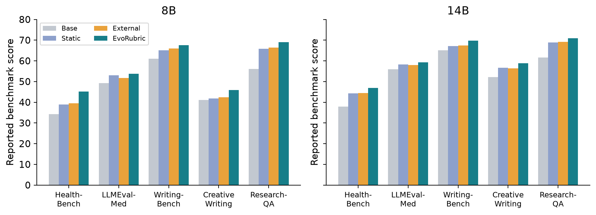
Figure 5. Replot of paper Table 1 means. The bars omit uncertainty for readability; the source table reports standard deviations over three runs. Five bars per method span three separately trained domain policies.

At 8B, the reported macro-average rises from 53.19 for the strongest matched average baseline to 56.28, a 3.09-point gain. At 14B, it rises from 59.07 to 61.13, a 2.06-point gain. EvoRubric has the highest reported mean in each benchmark at both scales.

The largest 8B gain over the strongest baseline in the corresponding column is HealthBench: $45.13-39.53=5.60$ points. LLMEval-Med gains $53.75-52.95=0.80$ points, where the strongest comparator is the static baseline. Picking the strongest comparator independently for each column is different from comparing every column only to External Evolving-RL.

The standard deviations matter. For instance, 8B LLMEval-Med is $53.75\pm0.84$ versus $52.95\pm0.47$. A consistent ranking of means is encouraging, but three training seeds and these summary statistics do not justify declaring every column statistically decisive. Prompt-level dependence and evaluation noise also need attention.

6.2 What the macro-average weights

The average is an unweighted average over five benchmarks. Two are Medical, two are Writing, and one is Science. It therefore implicitly assigns 40%, 40%, and 20% to those domains. A domain-balanced average would answer a different question.

This weighting does not invalidate the reported result, but it shapes how to use it. An application dominated by scientific questions should inspect ResearchQA separately. A system that must preserve comprehensive explanations should examine the human completeness dimension rather than relying on a macro-average of benchmark scores.

6.3 Component ablations

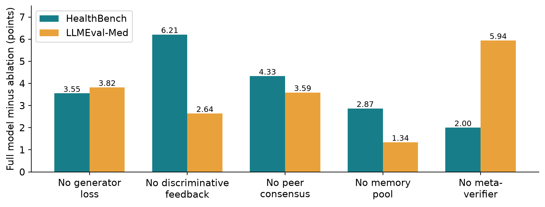
Figure 6. Full-model score minus each ablation, recomputed from paper Table 2. These are conditional removal effects, not additive allocations of the total improvement.

Removing the Generator loss drops HealthBench by 3.55 points and LLMEval-Med by 3.82. Rubric sampling, verification, grading, memory, and selection remain active. Because the parameters are shared, rubric behavior can still change indirectly through Reasoner updates. The ablation therefore supports the value of explicit Generator optimization beyond that indirect change.

Removing discriminative feedback produces the largest HealthBench drop among the listed variants, 6.21 points. Removing the Meta-Verifier produces the largest LLMEval-Med drop, 5.94 points, taking the result below the untrained base score on that benchmark. Removing consensus or memory also lowers both means.

It would be incorrect to add those drops and call the sum a contribution budget. Each intervention changes the environment seen by the other mechanisms. For example, consensus over unverified criteria is a different signal from consensus over screened criteria. The ablations show that the assembled design benefits from each part under the tested setup; they do not isolate globally independent causal effects.

6.4 A stronger external generator

In Medical, replacing the frozen same-scale external generator with GPT-4.1 improves HealthBench from 39.53 to 42.25 and LLMEval-Med from 51.73 to 52.92. EvoRubric still reaches 45.13 and 53.75. This suggests that learning criterion generation can outperform simply increasing external generator capability in this controlled setting.

The comparison is a DR-Tulu-style criterion-generation strategy transplanted into the paper’s setup. It is not a comparison against the complete DR-Tulu search-and-citation system. Appendix A explicitly preserves that boundary.

Appendix H reports 81.20 million input tokens and 2.91 million output tokens per run for the GPT-4.1 generator variant, approximately $185.70 under the experiment’s pricing. That is generator API expenditure only. It excludes other grading, training, hardware, and operational costs, so it cannot establish an end-to-end cost advantage by itself.

7. Do the criteria and answers improve in the same way?

7.1 A successful safeguard still has residual drift

Three annotators with medical-rubric experience audited the same twenty Medical prompts over four epoch-end snapshots. At the final 8B snapshot, eight of 157 pool entries are invalid; without the verifier, 75 of 192 are invalid. The relative reduction computed from the integer counts is

$$1-\frac{8/157}{75/192}\approx0.8696. \tag{15}$$

This is an 86.96% relative reduction in invalid-entry rate, not an 86.96 percentage-point improvement. It is also a comparison between two evolving pools with different denominators, rather than a paired set of exactly the same criteria screened in two ways.

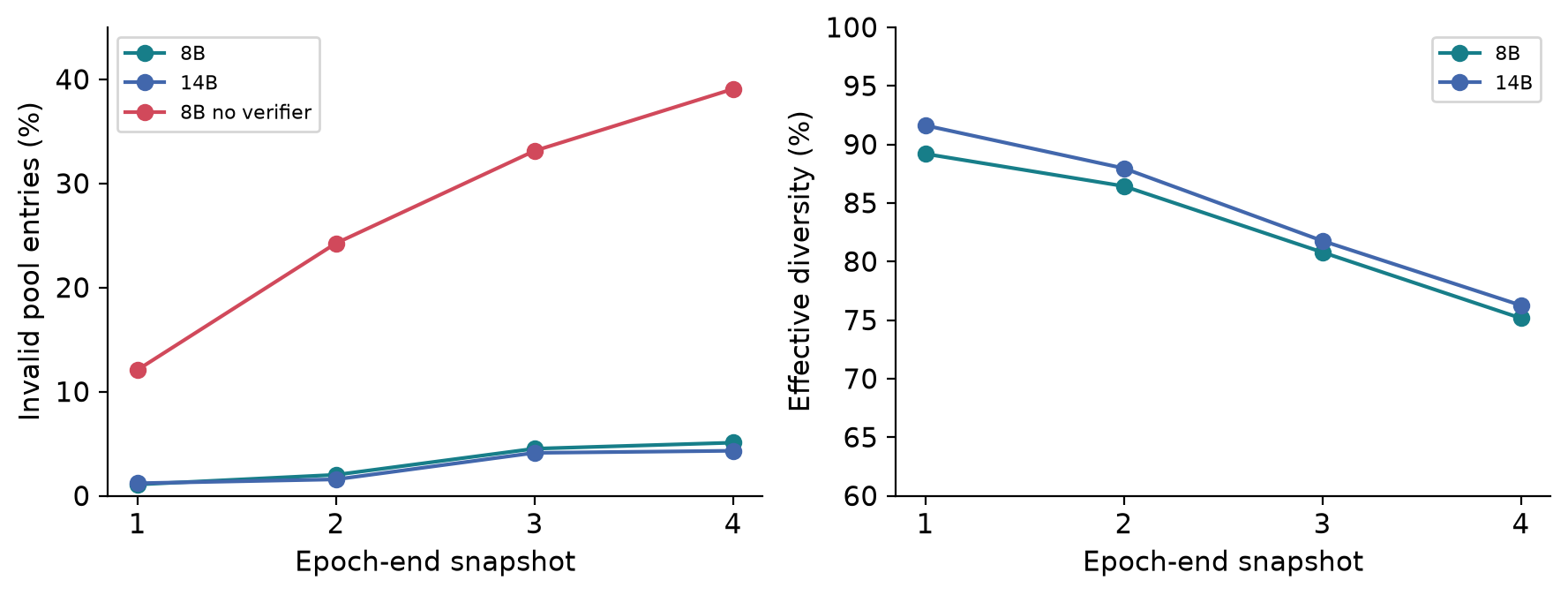
Figure 7. Ratios recomputed from paper Tables 9 and 10. Invalidity rises and effective diversity falls across training even with the verifier. The changing denominators are retained in the calculations.

With verification, the 8B invalid rate still rises from 2/185 at the first snapshot to 8/157 at the fourth. The 14B trajectory also ends above its initial rate. The relevant conclusion is that verification substantially limits error accumulation in this audit, not that it eliminates it.

Effective diversity is the number of human-valid, semantically distinct dimensions beyond base criteria, divided by all entries in the pool. Equivalence is resolved within each prompt; criteria across different prompts are not globally deduplicated. At 8B it falls from 165/185, or 89.19%, to 118/157, or 75.16%. A final pool can remain mostly valid while its novelty and diversity decline.

The final 8B pool contains 149 valid entries but only 118 distinct valid dimensions beyond the base. Those counts measure different things. “Valid” does not imply “new,” and “new” does not imply that every valid entry contributes a separate dimension. Reporting only validity would miss that distinction.

7.2 Human preferences reveal a tradeoff

The blind response comparison uses fifty Medical prompts and three annotators. Majority judgments determine prompt-level wins, ties, and losses; a three-way split is recorded as a tie. The same-scale external comparison gives overall quality 42/30/28, and the GPT-4.1-generator comparison gives 48/14/38.

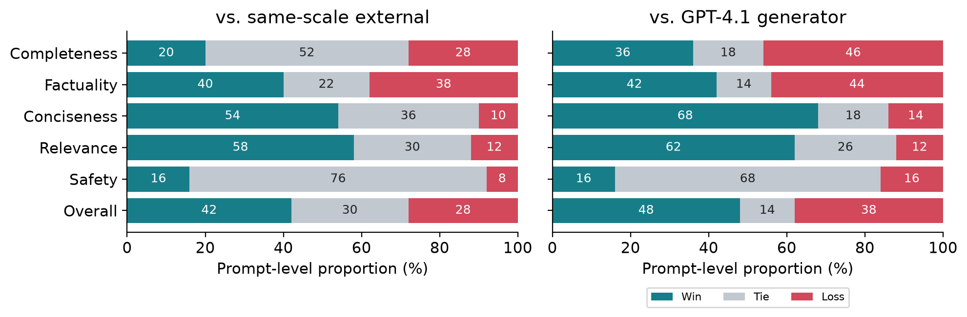
Figure 8. Paper Table 6, including ties. Wins favor EvoRubric. The clearest advantages are conciseness and relevance; completeness more often favors the comparators.

Removing ties yields $42/(42+28)=60\%$ and $48/(48+38)\approx55.8\%$. These are non-tie win rates, not the fraction of all prompts won. In counts, the overall outcomes are 21 wins, 15 ties, 14 losses against the same-scale external model, and 24 wins, 7 ties, 19 losses against the stronger generator variant.

The dimension-level pattern is more informative than the headline. Conciseness and relevance favor EvoRubric strongly. Completeness favors the baselines more often. Factual correctness is nearly balanced, and safety is mostly tied. The paper consequently supports a quality tradeoff with modest overall preference gains, not an across-the-board human judgment of superiority.

The length penalty makes this pattern especially interesting. It may help remove redundant text while also discouraging useful elaboration. The paper does not isolate how much of the human preference profile comes from length shaping versus criterion learning. A matched response-length analysis would help distinguish these explanations.

7.3 Controlled rubric quality and initialization

On one hundred fixed query-response groups, the model-based evaluator prefers EvoRubric’s criteria 72% of the time over the same-scale external generator’s 28%. Holding responses fixed is a useful control: a generator cannot win this comparison simply because it was shown better answers. However, the judgment still reflects the chosen evaluator’s notions of professionalism, granularity, and discrimination.

Expert initialization raises static-rubric HealthBench from 38.89 to 41.83. Applying co-evolution with expert rubrics raises it further to 44.64. Model-initialized EvoRubric reaches 45.13. The small 0.49-point difference between those two evolving variants is not grounds to dismiss expert priors generally.

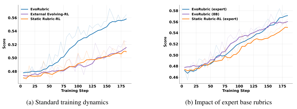
Figure 9 (paper Fig. 3). Training trajectories are scored by GPT-OSS-120B using base rubrics held fixed within each initialization setting. They are not the independent final-evaluator scores in Table 1.

A fixed scoring target makes the trajectory interpretable as progress against that target while memory changes. It remains possible to improve against a fixed grader’s blind spots, however. The separate final evaluator and human judgments therefore add evidence that the training curve alone cannot supply.

8. Practical reading of the training specification

Appendix E reports four epochs, batch and minibatch size 64, microbatch size 16 per GPU, learning rate $10^{-6}$ with a constant schedule, AdamW, and eight NVIDIA H20 GPUs. Sampling uses temperature 0.7, top-p 0.8, and top-k 20. Maximum prompt length is 12,288 and maximum response length 8,192.

The Generator prompt can include eight answers, base criteria, and historical memory. Eight answers near the maximum response length cannot all fit unabridged within the stated prompt limit. The main text explicitly qualifies access to sampled answers by the input budget. The precise treatment of that budget can affect which differences the Generator observes and deserves explicit reporting in future comparisons.

A useful estimate of scoring work is proportional to $N$ times the total number of base, historical, and verified current criteria. With eight answers and four proposed rubric sets, grading work can exceed answer rollout work in ways a simple “one shared policy” description conceals. Batching calls may improve throughput, but does not change the logical amount of answer-criterion evaluation.

Memory is keyed by query, which makes repeated visits valuable. If every training query is encountered only once, the historical channel cannot provide the same benefit. If prompts are slightly paraphrased and treated as separate keys, knowledge need not transfer through memory even when the policy generalizes. This is a property of the design, not evidence that the reported four-epoch setting is ineffective.

For a faithful empirical comparison, I would record criterion proposals before and after screening, batch eligibility rates, constant-score groups, memory survival times, role-specific token counts, and all evaluator identities. Those records would reveal whether a gain reflects richer criteria, different sample lengths, or a changing proportion of informative groups. They are suggested experimental measurements, not claims of measurements performed here.

9. Limitations

The principal limitation is epistemic: agreement among self-generated evaluators cannot by itself establish correctness. The frozen validity checker is an imperfect anchor. The twenty-prompt audit demonstrates residual errors and declining effective diversity even under the full method.

The strongest human evidence is limited to fifty Medical prompts. Writing and Science are assessed through benchmarks and model judgments, without the same reported human response audit. Domain-specific training also limits claims about a single general model acquiring broad transferable rubric expertise.

Only three training seeds are summarized. Some benchmark differences are small relative to reported variation. The audit pools criteria within prompts, so treating all entries as independent observations would overstate precision. A broad claim about reliability would need more prompts, independent annotator cohorts, and explicit uncertainty.

The base rubric remains fixed, which is helpful as an anchor but can preserve omissions or errors. An evolved memory capped at ten entries may forget useful rare requirements, while exact-match insertion does not fully prevent semantic redundancy. FIFO replacement is simple but does not explicitly optimize long-term coverage.

Finally, the study does not establish end-to-end efficiency at equal total supervisory compute. The external generator cost is only one component. Shared policy training, large-model grading, meta-verification, and evaluation all consume resources. Performance improvements and resource savings should be established separately.

10. Critical analysis: the next experiments I would prioritize

10.1 Test disagreement that is correct

LOO consensus rewards alignment with peer score patterns. I would construct a held-out set where one valid minority criterion identifies a consequential error overlooked by the other batches. The central measurement would be the probability that the minority criterion survives screening, crosses the eligibility threshold, and reaches memory.

A useful alternative is to retain a small disagreement budget: preserve one valid, high-impact dissenting criterion alongside the consensus winner. That would sacrifice some noise reduction to protect novel discoveries. It should be judged by held-out error detection and human validity, not merely by increased rubric diversity.

10.2 Test whether retired skills regress

Saturation is estimated from eight current samples. If a failure has probability $p$ and samples were independent, the probability of seeing no failures would be $(1-p)^8$. For $p=0.1$, this is about 0.43. A failure mode could therefore look mastered in a small group even when it remains material. Real samples can be correlated, so this independence calculation is illustrative rather than a guarantee.

I would retain a compact archive of retired criteria and periodically reevaluate them on fresh responses. Regression-triggered reactivation would preserve memory capacity for new distinctions while preventing retirement from becoming irreversible forgetting. Compare it with FIFO at equal active capacity and equal evaluation budget.

10.3 Separate criterion importance from ease of discrimination

A rule can split responses because it measures a meaningful error, or because it measures an irrelevant stylistic detail. Meta-verification screens the latter in principle, but the scoring incentives still favor detectable variation. Important rules that all answers fail can remain silent under group-relative learning.

One possible extension is a two-channel objective: retain relative reward for discriminative criteria, and add a separately calibrated signal for severe unanimous failures. Such a signal would require stronger external grounding and could introduce its own bias. Its purpose would be to address a specific weakness of relative comparison, not to claim that any additional reward is automatically beneficial.

10.4 Measure the complete quality-cost frontier

I would compare fixed, external evolving, and shared-policy rubrics at matched total grader tokens, meta-verifier tokens, rollout tokens, and accelerator time. Report performance against cost rather than only against training steps. Include a condition that spends saved Generator resources on more diverse response samples.

The same experiment should stratify human judgments by response length. If conciseness gains remain after length matching while completeness no longer drops, that would strengthen the argument for improved criteria. If the gains disappear, the method may primarily be learning a useful but narrower presentation preference.

10.5 Audit meaning, not only acceptance

The audit already exposes a gap between validity and effective diversity. I would extend it to track criterion lineages: which new rule replaced which retired rule, whether it introduced a genuinely new failure dimension, and whether its downstream effect transferred to unseen prompts. That would connect the memory mechanism to learning rather than treating memory growth as progress.

The most persuasive evidence would be a blind held-out error taxonomy created independently of the training criteria. Improved coverage of that taxonomy, coupled with stable or improved human answer quality, would make “self-evolving supervision” a more concrete empirical claim.

11. Conclusion

EvoRubric offers a coherent way to train criterion discovery when open-ended tasks lack a definitive final-answer target. The same policy learns to answer and to articulate missing standards, while frozen validity checking, grading, peer agreement, and per-query memory constrain the feedback loop.

I find the separation of validity, discrimination, and consensus more useful than the broad label of self-evolution. It makes the design inspectable: one can ask which criteria are acceptable, which distinguish current answers, which agree with peers, and which survive into future training.

The reported gains across five benchmarks are supported by ablations and additional audits. The human results and pool dynamics also prevent an overly simple success story. Better relevance and conciseness coexist with weaker completeness preferences, residual invalid criteria, and decreasing effective diversity. The next step is to show that adaptive standards continue to improve independently measured quality as their own feedback becomes increasingly optimized.

References

1. Xin Guan et al. EvoRubric: Self-Evolving Rubric-Driven RL for Open-Ended Generation, v2. Main source for all reported results and method details; Sections 3-4, Tables 1-10, and Appendices A-J.
2. Zhihong Shao et al. DeepSeekMath: Pushing the Limits of Mathematical Reasoning in Open Language Models. Background reference for GRPO, as cited by EvoRubric.
3. Rulin Shao et al. DR Tulu: Reinforcement Learning with Evolving Rubrics for Deep Research. Related-method pointer; the comparison discussed here is EvoRubric’s controlled external-generator variant.
4. Leheng Sheng et al. Reinforcing Chain-of-Thought Reasoning with Self-Evolving Rubrics. Related-method pointer for correctness-referenced rubric learning discussed in EvoRubric Appendix A.