Dobi-SVD: What Changes When We Compress Activations Before We Compress Weights?

Review date: 2026-10-16
Paper reviewed: Dobi-SVD: Differentiable SVD for LLM Compression and Some New Perspectives
Paper authors: Qinsi Wang, Jinghan Ke, Masayoshi Tomizuka, Yiran Chen, Kurt Keutzer, Chenfeng Xu
Identifier and version: arXiv:2502.02723v1, 2025-02-04
Resources: Paper and appendices · Author project page · Official resource entry

1. Three decisions hidden inside one compression ratio

The useful question in low-rank model compression is not simply how many singular values to discard. It is which space supplies those singular values, how a single set of weights can serve many inputs, and how much precision each retained component deserves. Dobi-SVD puts all three decisions into the same framework. It first learns where to truncate the activations of different linear layers, then constructs fixed weights from the resulting subspaces, and finally lowers the storage precision of selected factor blocks so that more rank fits into the same byte budget.

This ordering explains both the strength and the difficulty of the paper. The best rank-constrained approximation of one activation matrix has a clean mathematical answer. A deployable language model, however, cannot store a separate weight matrix for every calibration example. It needs one fixed approximation that continues to work on unseen prompts. Moving from the first statement to the second introduces an aggregation problem that the local optimality theorem does not settle. Likewise, doubling the number of retained components at a given storage budget is possible only after changing another resource: numerical precision.

My reading is that Dobi-SVD is a useful proposal for jointly choosing rank and representation, with an especially instructive distinction between calibration-time activation truncation and inference-time factorized weights. Its strongest evidence concerns the quality of the combined method on the evaluated models. Its broader claims about optimal weight reconstruction and universal superiority require more qualification. Those qualifications are not peripheral: they explain which parts can transfer to a new compression design and which parts must be established again.

Throughout this review, a smaller retained ratio means more compression. A retained ratio of 0.4 means a nominal 40% resource budget, or 60% removed. Before remapping, the paper counts factor entries relative to dense entries. After remapping, the equivalent expression counts bit storage relative to the original precision. I will keep these meanings separate. All experimental numbers below come from the paper; the small matrices and analytical plots are constructed explanations, not measurements on a language model.

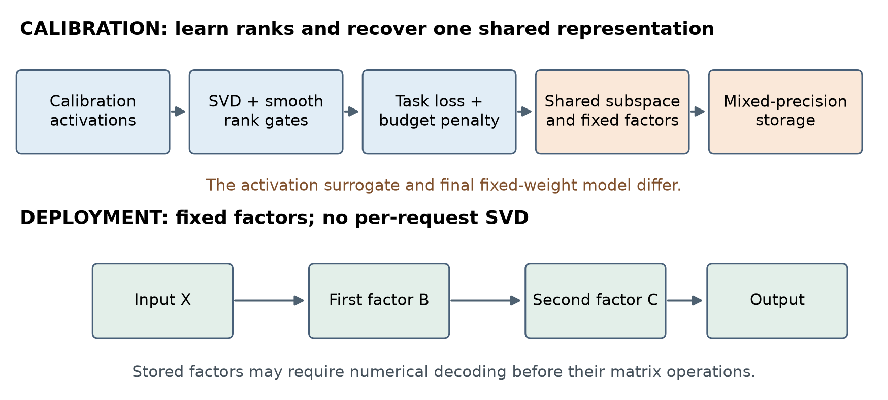
Figure 1. Original conceptual overview of Sections 3.1–3.3. Calibration uses activation decompositions and task feedback; deployment uses recovered fixed factors. The diagram separates these phases without prescribing a particular runtime kernel.

2. Prerequisites: rank, activations, and the metric that matters

2.1 Fix the dimensions before interpreting the decomposition

Use row-oriented inputs. Let $X\in\mathbb{R}^{t\times m}$ contain token representations, let $W\in\mathbb{R}^{m\times n}$ be a linear layer, and let $A=XW\in\mathbb{R}^{t\times n}$ be its output. A rank-$k$ factorization stores $B\in\mathbb{R}^{m\times k}$ and $C\in\mathbb{R}^{k\times n}$, so inference computes $(XB)C$. This convention makes the right singular vectors of the activation matrix directions in the output feature space. It also prevents confusing a token-space projection with an output-channel projection.

For a thin singular value decomposition, $A=U\Sigma V^\top$, the columns of $U$ and $V$ are orthonormal. This is orthogonality, not a claim that either rectangular factor is a positive-definite matrix. The singular values are nonnegative and ordered. Rank counts independent directions, while the magnitude of a singular value measures how much energy appears along one direction under the chosen matrix norm.

The Frobenius norm sums squared entry errors. It treats every coordinate in the matrix being approximated equally. That last phrase matters: treating errors in $W$ equally is different from treating errors in $XW$ equally. Inputs can amplify a small weight direction or almost never excite a large one. A low-rank method therefore needs an explicit error metric before any claim of optimality has meaning.

2.2 Why a weight-optimal approximation can be activation-poor

Let $E=W-\widehat W$. The squared activation reconstruction error expands as

$$\begin{aligned} \|X(W-\widehat W)\|_F^2 &=\operatorname{tr}(E^\top X^\top X E)\\ &=\|H^{1/2}E\|_F^2,\qquad H=X^\top X. \end{aligned}\tag{1}$$

The first line follows by substituting $XE$ into the definition of the Frobenius norm and collecting the middle factors. The second line uses a positive-semidefinite square root of the input Gram matrix. This derivation shows exactly what ordinary weight SVD neglects: the geometry imposed by $H$. If $H$ is proportional to the identity, the two objectives agree up to scale. With strongly anisotropic inputs, they can disagree sharply.

Consider an illustrative two-dimensional layer with $W=\operatorname{diag}(3,1)$ and $X=\operatorname{diag}(1,10)$. Weight SVD at rank one preserves the first coordinate because 3 exceeds 1. But $A=\operatorname{diag}(3,10)$, so activation SVD preserves the second. The weight-selected output has squared reconstruction error 100; the activation-selected output has error 9. No language-model training is involved in this example. It simply exposes why a model’s weight spectrum alone need not identify the directions most useful on its inputs.

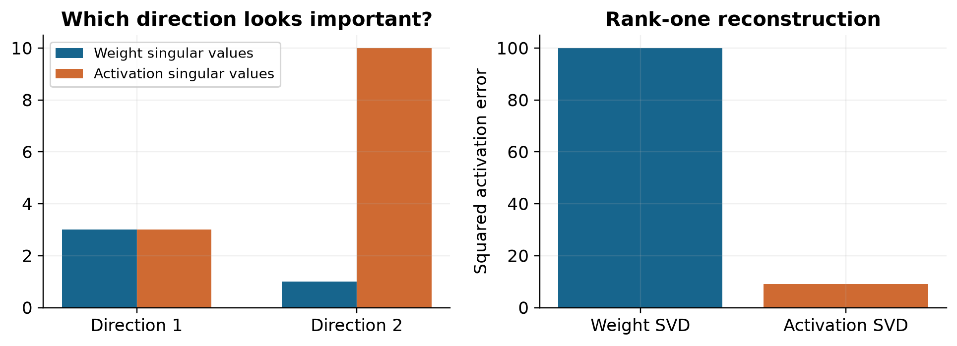
Figure 2. Analytical example with diagonal $X$ and $W$. The bars show squared activation errors, not model benchmark results. Weight SVD minimizes a different objective from activation SVD.

An important alternative follows directly from Equation (1): if the input Gram matrix can be handled stably, one can whiten the input-weight geometry, truncate in that space, then map back. Thus activation truncation is not the only route to an activation-aware objective. The practical comparison involves covariance conditioning, calibration cost, the chosen approximation family, and how rank is allocated across layers. It is too strong to conclude that all methods operating through weights are inherently unable to minimize activation error.

2.3 A norm guarantee is not a task-loss guarantee

The Eckart–Young–Mirsky theorem identifies a best rank-$k$ approximation under the Frobenius or spectral norm. It does not say that the same approximation minimizes next-token cross-entropy, code-generation failures, or a robot’s task failure rate. A coordinate with small activation energy can still have a large downstream loss derivative. This distinction will reappear in the critique of the paper’s model-level argument.

There is still a good reason to use reconstruction error. It is measurable with modest calibration data and gives a controlled local target. The caution is about interpretation: reconstruction is a surrogate for behavior. Gradient-guided rank selection can make that surrogate more responsive to the task, but the eventual fixed-weight reconstruction and quantization introduce additional approximation stages after rank learning.

3. The exact bridge from one activation to one weight matrix

Let $V_k$ contain the top $k$ right singular vectors of $A$, and define $P_k=V_kV_k^\top$. This is an orthogonal projector in $\mathbb{R}^n$. Multiplying on the right by this projector retains precisely the selected output directions:

$$\begin{aligned} A_k&=U_k\Sigma_kV_k^\top=AV_kV_k^\top\\ &=XWV_kV_k^\top=X\widehat W_k,\\ \widehat W_k&=WV_kV_k^\top,\qquad \operatorname{rank}(\widehat W_k)\le k. \end{aligned}\tag{2}$$

The key step is associativity. We never invert $X$. Even when there are fewer calibration tokens than input channels, or when $X$ is rank-deficient, this construction reproduces $A_k$ on that batch. The factorization is already available: $B=WV_k$ and $C=V_k^\top$. These factors can be stored and applied to future inputs using two ordinary linear maps.

For this fixed $X$, any rank-$k$ weight matrix produces an activation of rank at most $k$. Equation (2) supplies a feasible weight matrix that achieves the best rank-$k$ activation. Therefore it attains the minimum activation reconstruction error over this weight family. If the activation has enough nonzero singular directions and the retained singular values are positive, the constructed weight has rank $k$; the safe general statement is rank at most $k$.

This result is stronger than merely saying that activation SVD is a useful heuristic. It is an exact statement about a particular batch, a particular linear map, and a particular norm. Its limits are equally precise. The weight matrix need not be unique: any component in the input null space is invisible on the calibration batch. More importantly, the projector depends on the input distribution. A projector that is ideal for one batch need not be ideal for another.

3.1 Why activation SVD is a calibration device

A reader might initially imagine recomputing an SVD at every inference token. That would be a different method with a very different cost profile. In Dobi-SVD, the activation-side operation supplies calibration signals and candidate subspaces. The final deployment object is a set of fixed factors. The expensive activation decomposition should therefore be assessed as part of compression cost, while the two factor multiplications and any precision conversion belong to inference cost.

This separation matters when an experiment reports only a small number of trainable parameters. Learning one scalar rank control for each matrix saves optimizer state relative to updating billions of weights. It does not eliminate forward activations, matrix decompositions, or backward propagation through the network. The size of the trainable vector and the cost of finding it are related only indirectly.

3.2 A stacked-data alternative clarifies the target

If all calibration activations could be stacked into $A_{\mathrm{stack}}=[A_1;\ldots;A_N]$, an SVD of this matrix would find an energy-weighted output subspace for their joint reconstruction. Equivalently, the right directions come from the leading eigenspace of $\sum_i A_i^\top A_i$. This observation does not prescribe materializing a huge stack. It clarifies that averaging batch subspaces, retaining activation magnitudes, and minimizing original task loss are three different objectives.

In particular, a subspace-only summary gives a weakly excited batch the same directional vote as a strongly excited one if both contribute the same number of basis vectors. That can be a deliberate robustness choice, but it is not automatically the optimizer of the activation-energy objective. A good compression analysis should say which information has been discarded between the original activations and the stored summary.

4. Learning the truncation boundary

4.1 Replace a discrete cutoff with a smooth gate

Integer rank cannot be optimized by an ordinary derivative. Dobi-SVD attaches a scalar cutoff $k$ to each matrix and replaces the hard keep/drop decision by a hyperbolic-tangent gate. For a singular component indexed by $i$,

$$g_i(k)=\frac{1+\tanh(\beta(k-i))}{2},\qquad \widetilde\sigma_i=\sigma_i g_i(k). \tag{3}$$

When $i$ lies well below $k$, the gate approaches one; well above $k$, it approaches zero. At the boundary it is one half. The positive parameter $\beta$ controls transition width. The paper uses $\beta=10$. A large value resembles a hard cutoff, but it also concentrates useful derivatives into a narrow region. A small value sends gradient information across more components while making the forward representation less like the eventual discrete rank.

Differentiating the gate gives

$$\frac{\partial\widetilde\sigma_i}{\partial k} =\frac{\beta\sigma_i}{2}\operatorname{sech}^2(\beta(k-i)). \tag{4}$$

The derivative is largest near the cutoff and is scaled by the singular value itself. This provides an intuitive reading of the update: rank moves when retaining or suppressing nearby spectral components helps the task enough to justify their storage cost. It does not independently select an arbitrary subset of components. The gate preserves a monotone spectral ordering and learns a boundary within that ordering.

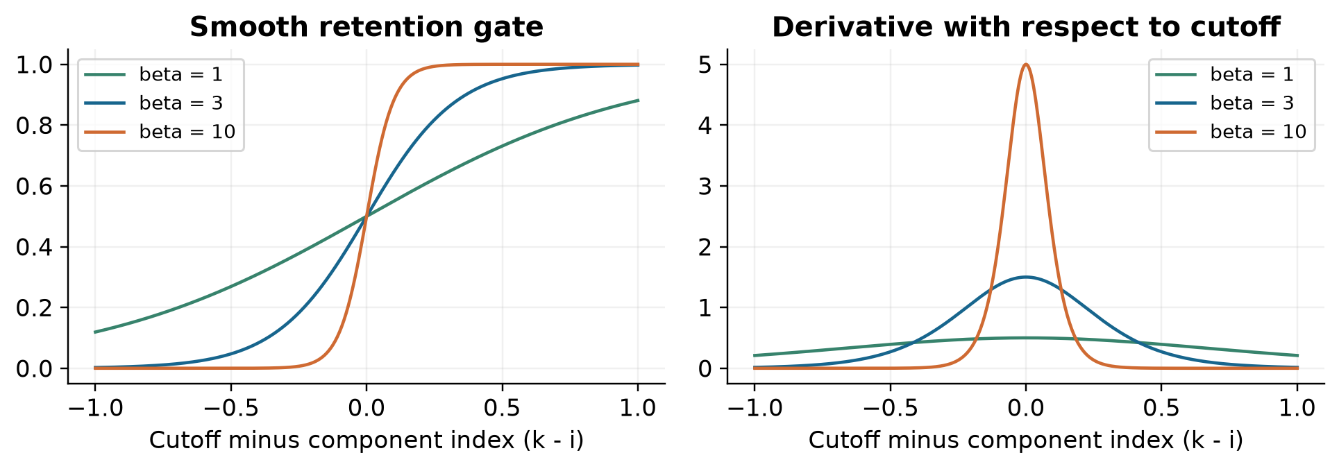
Figure 3. Analytical plots of the gate and its derivative for several smoothing strengths. These show the tradeoff between a sharp rank decision and a broad region with useful gradients.

4.2 Task loss and the global budget

For rank controls $\{k_\ell\}$, the training objective combines task loss with a penalty for departing from the target retained ratio:

$$\mathcal L=\mathcal L_{\mathrm{task}} +\lambda\left|R(\{k_\ell\})-R_{\mathrm{target}}\right|. \tag{5}$$

I use $\lambda$ for this penalty coefficient because the paper also uses $\gamma$ in its numerical-stability discussion. They are different roles and should not be treated as one hyperparameter. If the unquantized factor cost of matrix $\ell$ is $c_\ell k_\ell$, where $c_\ell=m_\ell+n_\ell$, a natural aggregate ratio is $\sum_\ell c_\ell k_\ell/\sum_\ell m_\ell n_\ell$. A byte-aware remapped objective must use its corresponding storage costs instead.

This makes a useful resource-allocation interpretation possible. Increasing a rank is worthwhile when its marginal reduction in task loss exceeds its marginal budget penalty. Equal ranks or equal rank percentages cannot generally satisfy that balance across matrices of different shapes and sensitivities. The learned cutoff gives each matrix a continuous way to negotiate for capacity.

The penalty is not a hard feasibility guarantee. Finite optimization, nonsmooth absolute value at the target, and later rounding can leave a mismatch. For an actual compression result, one must distinguish the continuous target from the discrete model’s achieved byte count. A rank rounded up in a large feed-forward matrix can cost more than the same numerical increment in a smaller attention matrix. Merely preserving the sum of ranks does not always preserve storage.

Algorithm 1. Conceptual differentiable rank selection

Input: fixed model weights, calibration data, target budget
1. Give each compressed matrix a continuous rank control k.
2. For each calibration batch, compute layer activations.
3. Decompose each selected activation and gate its singular values.
4. Propagate the gated activations through the remaining model.
5. Form task loss plus a penalty for the current representation cost.
6. Backpropagate through the activation path; update only rank controls.
7. Repeat, then obtain feasible integer ranks for fixed-weight recovery.
Output: one target rank per compressed matrix

This pseudocode summarizes the paper’s optimization idea. The feasibility check in the last step is an explicit practical requirement of using integer factors, rather than a claim that the source provides a complete budget-rounding algorithm. The distinction matters because the learned continuous representation is only an intermediate object.

4.3 Few variables can still mean substantial work

The paper reports 224 trainable rank parameters for LLaMA-7B and an eight-GPU-hour training statement. Appendix A.3 specifies 256 WikiText-2 samples of 2,048 tokens, batch size 32, 320 epochs, Adam, a cosine schedule, and learning rate 0.1. Those details make clear that this is an optimization procedure using data, even though the original weights are frozen. Describing it simply as having no training would conceal the dominant calibration process.

A distinction worth preserving is that the later weight reconstruction stage does not require additional weight fine-tuning. That is compatible with rank learning having a nonzero training cost. When comparing with a method that computes a single covariance and truncates once, the meaningful quantities include total compression time, peak memory, calibration size, and the quality of the final model at the same storage target. Trainable-parameter count alone is not an adequate cost comparison.

5. Stable SVD differentiation: a controlled approximation

Singular vectors become poorly determined when two singular values nearly coincide. A rotation within the almost-degenerate subspace can change the individual vectors substantially while changing their spanned subspace very little. Derivatives written in terms of those individual vectors therefore contain inverse spectral gaps. This is a structural issue, not merely an optimizer taking an overly large step.

For two positive singular values $a>b$, consider the positive magnitude of the gap kernel:

$$\begin{aligned} C(a,b)&=\frac{1}{a^2-b^2} =\frac{1}{a^2}\frac{1}{1-q^2},\qquad q=b/a,\\ C_N(a,b)&=\frac{1}{a^2}\sum_{j=0}^{N-1}q^{2j}. \end{aligned}\tag{6}$$

The geometric expansion is valid for $|q|<1$. Keeping a finite number of terms prevents the expression from diverging as $q$ approaches one: its limit is $N/a^2$. The omitted tail for distinct values is

$$C-C_N=\frac{q^{2N}}{a^2(1-q^2)}. \tag{7}$$

This is a useful way to understand what stabilization purchases. It bounds the near-collision response at a given scale, but it deliberately biases the exact inverse-gap expression near that collision. If both singular values are close to zero, even $N/a^2$ is large. A separate small-value treatment is therefore needed. Dobi-SVD discusses thresholding and special handling for this case; the appendix lists a small-value parameter of $10^{-10}$ and ten Taylor terms.

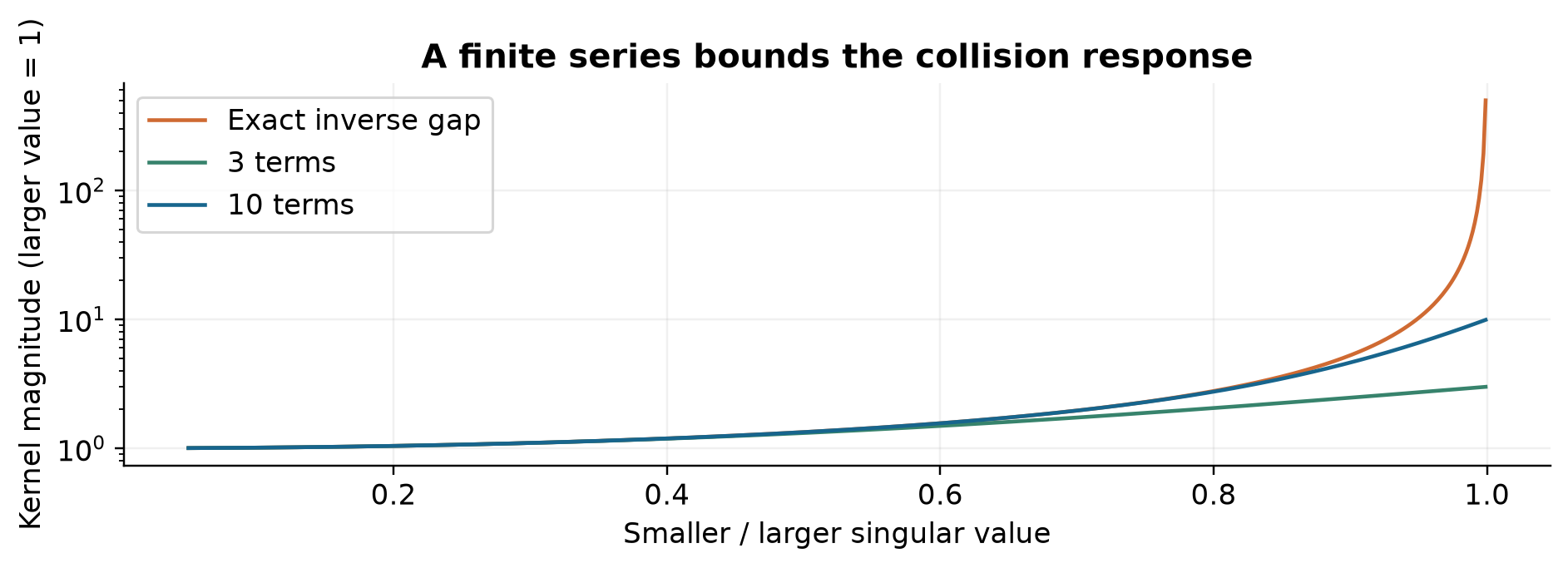
Figure 4. Analytical illustration with the larger singular value normalized to one. A finite series limits the collision response; it is not an exact derivative at repeated singular values.

The main text and Appendix Algorithm 5 express the expansion in different forms. The sign convention for the printed gap also changes between the main equations. Equation (6) above deliberately uses a positive magnitude so that its convergence and approximation error are unambiguous. A full matrix derivative must additionally respect the antisymmetric ordering of index pairs, orthogonal-complement terms for rectangular factors, and the special treatment of zero values. The scalar derivation should not be copied as if it were a complete backward rule.

An alternative is to optimize a quantity defined directly on a projector or a spectral function, where arbitrary rotations inside a repeated-value subspace may cancel. That can improve the mathematical representation of the objective, but it does not by itself solve rank changes at a cutoff. Another alternative is a search over discrete ranks, avoiding differentiation through the SVD while paying for candidate evaluations. Dobi-SVD’s choice is attractive when task-guided continuous optimization provides enough quality to justify the decomposition and stabilization cost.

The important failure boundary is a cutoff through a cluster of near-equal singular values. In that region, a tiny perturbation can change which individual vector is counted as the last retained component. A stable numerical update is useful, but it does not prove that a particular discrete basis is intrinsically meaningful. A careful interpretation should emphasize the resulting subspace and task behavior, rather than attaching too much significance to an individual singular vector.

6. Many inputs require a shared subspace

6.1 What is being aggregated?

For calibration batch $i$, let $V_i$ denote the retained activation basis and $P_i=V_iV_i^\top$ its projector. Each batch suggests the weight matrix $WP_i$. A deployed layer needs a common projector $P=VV^\top$. A direct objective would retain the input weighting:

$$J_X(V)=\sum_i\|X_iW(P_i-VV^\top)\|_F^2, \qquad V^\top V=I_k. \tag{8}$$

This expression measures the discrepancy between each batch’s desired truncated activation and the shared weight’s output on that batch. Removing $X_i$ changes the metric. Removing $W$ as well changes it again. The main paper’s Equation (5) writes a matrix outside a norm in a way that should not be read as a scalar norm identity. In general, $\|X_iE\|_F$ cannot be replaced by $X_i\|E\|_F$.

Appendix A.4.1 instead studies a weight-space discrepancy and upper-bounds it by an unweighted projector discrepancy. The useful, well-defined surrogate is

$$J_P(V)=\sum_i\|P_i-VV^\top\|_F^2. \tag{9}$$

For rank-$k$ orthogonal projectors, $P_i^2=P_i$, $P^2=P$, and each trace is $k$. Expanding the norm therefore gives

$$\begin{aligned} J_P(V) &=2Nk-2\sum_i\operatorname{tr}(P_iVV^\top)\\ &=2Nk-2\operatorname{tr}(V^\top S V), \qquad S=\sum_iP_i. \end{aligned}\tag{10}$$

Minimizing this surrogate is equivalent to maximizing the last trace over orthonormal columns of $V$. The leading $k$ eigenvectors of $S$ solve that problem. If $Z=[V_1,\ldots,V_N]$, then $ZZ^\top=S$, so the leading left singular space of this horizontal stack gives the same answer. This is the concrete connection to principal-subspace estimation.

6.2 Why the bound does not transfer the optimizer

For the weight-space version, submultiplicativity supplies the bound

$$\sum_i\|W(P_i-P)\|_F^2 \le \|W\|_2^2\sum_i\|P_i-P\|_F^2. \tag{11}$$

The paper uses a Frobenius-norm bound, which is also valid but can be looser. Neither version says that the minimizer on the right minimizes the expression on the left. A constant upper bound on a family of functions does not establish equality of their optimizers. If $W$ stretches different output directions by very different amounts, a directional vote alone can give capacity to the wrong part of the space.

Here is a small counterexample to that transfer of optimality. Set $W=\operatorname{diag}(1,\sqrt{10},\sqrt{10})$ and retain one shared direction. Seven desired projectors point along coordinate axes: two along $e_1$, three along $e_2$, and two along $e_3$. The unweighted objective selects $e_2$, the most frequent direction, with cost 8; the other two choices each cost 10. The weight-space objective instead has costs 55, 62, and 82 for $e_1,e_2,e_3$, so $e_1$ is better.

This is not merely a comparison among three arbitrary candidates. For any unit direction $v$, the unweighted objective is $10v_1^2+8v_2^2+10v_3^2$, whereas the weight-space objective is $55v_1^2+62v_2^2+82v_3^2$. Since the squared coordinates sum to one, their respective global minima are attained at different axes. The counterexample concerns the two mathematical objectives; it does not assert that Dobi-SVD produces a particular error on a language model.

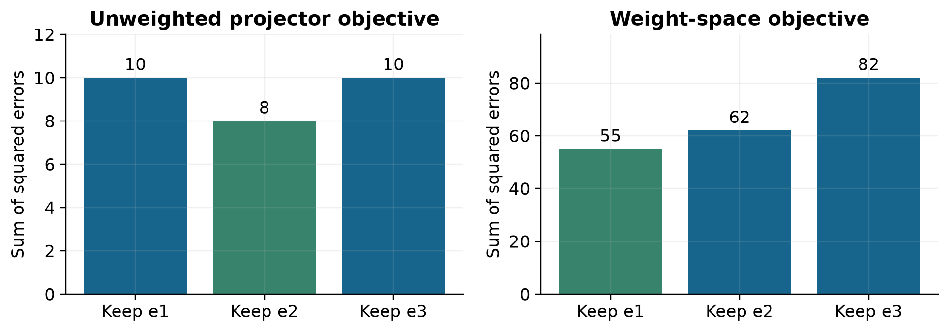
Figure 5. Seven constructed rank-one projectors in three dimensions. The unweighted projector objective and the weight-space objective select different shared directions. The two panels use their respective objective units.

6.3 What incremental PCA does and does not guarantee

The reason for using an incremental method is practical: carrying a summary of the important directions is cheaper than retaining all calibration bases. At each update, the current summary and a new batch’s information are combined, a decomposition is computed, and only the leading directions are retained. The state size depends on the retained dimension and feature dimension rather than the total number of stored examples.

That does not make memory independent of matrix dimension, and the paper’s plotted growth should not be promoted into a general exponential-versus-constant complexity theorem. Storing a dense covariance scales quadratically in feature dimension; storing a thin basis scales with feature dimension times retained rank. Which dominates depends on the specific incremental representation. Both remain substantial when the feature width and retained rank are large.

The source’s Algorithm 2, its prose, and its appendix motivate the same overall aggregation idea but leave details that matter mathematically: whether the stream consists of projected weights or singular-vector blocks, how centering is applied, whether singular-value magnitudes are retained in the summary, and what orientation is used in concatenation. A raw basis also has sign and rotation ambiguity. The projector is invariant to those changes, while centering the coordinates of a particular basis need not be.

Algorithm 2. Conceptual recovery of a fixed layer

Input: original W, calibrated rank k, activation data from many batches
1. For each batch, obtain a retained right activation subspace.
2. Accumulate a bounded-size summary of the shared directions.
3. Use a leading rank-k subspace V from that summary.
4. Construct B = W V and C = transpose(V).
5. Represent the deployed layer by X -> (X B) C.
6. Evaluate the fixed factors on held-out calibration data.
Output: fixed factors B and C, with no per-request SVD

This deliberately describes the recovery stage without inventing missing choices in the paper’s incremental pseudocode. An exact eigensolver for $S$ would solve Equation (9); a streaming approximation can deviate from that result after intermediate truncation. Even exact solution of Equation (9) remains a surrogate for Equation (8). These are two separate approximation boundaries, and distinguishing them is more informative than treating every stage as theoretically optimal.

7. Remapping is a rank–precision tradeoff

7.1 The factor-storage threshold

At unchanged precision, storing two factors for an $m\times n$ matrix requires $k(m+n)$ entries. The retained storage ratio is

$$\rho_{\mathrm{factor}}=\frac{k(m+n)}{mn}. \tag{12}$$

For a square matrix of width $d$, this is $2k/d$. Keeping half the rank uses the same number of entries as the original dense matrix; saving entries requires keeping less than half. This is a representation cost, not an impossibility theorem about encoding low-rank matrices. Lower precision, shared structure, or a different representation can change the cost. Dobi-SVD takes the first route.

For $m\ge n$, write the updated rank-$k$ matrix as a left factor $B\in\mathbb{R}^{m\times k}$ and right-factor transpose $V\in\mathbb{R}^{n\times k}$. Starting from 16-bit storage, the method quantizes the first $n$ rows of $B$ and all of $V$ to 8 bits. The remaining $m-n$ rows of $B$ stay at 16 bits. Ignoring scales and other metadata, the total bit count is

$$\begin{aligned} S_{\mathrm{bits}} &=8nk+8nk+16(m-n)k\\ &=16mk,\\ \rho_{\mathrm{remap}} &=\frac{S_{\mathrm{bits}}}{16mn}=\frac{k}{n}. \end{aligned}\tag{13}$$

The other rectangular orientation is symmetric. In general, the idealized ratio is $k/\min(m,n)$. Two 8-bit values occupy the byte budget of one 16-bit slot; they are still two numerical values with their own dequantization interpretation. Packing is not a lossless way to place two arbitrary 16-bit numbers in one 16-bit number.

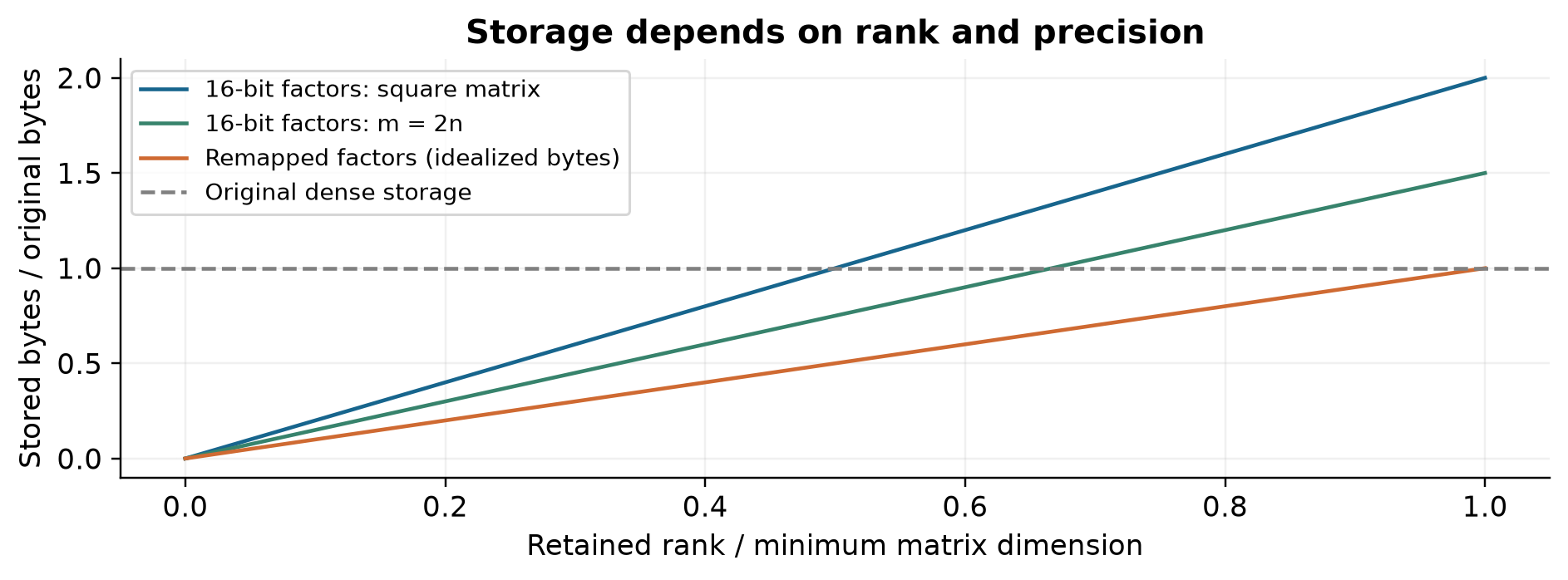
Figure 6. Analytical storage accounting for square and rectangular matrices, excluding quantization metadata. At the same byte ratio, remapping can retain more rank by lowering precision in selected factor blocks.

For a square 4,096-by-4,096 matrix, a nominal 0.4 retained-byte ratio corresponds to roughly 819 rank components with unchanged 16-bit factors, or roughly 1,638 with the idealized remapped representation. Integer rounding slightly changes the achieved ratio. The gain is that twice as many directions can be retained; the price is quantization error and the associated representation handling. This is a plausible bargain when discarded directions matter more than the small perturbations caused by quantization.

7.2 More retained rank can mean more arithmetic

The two dense factor multiplications require work proportional to $k(m+n)$ per token, regardless of how their values are packed on disk. Combining the remapped rank rule with this count gives the idealized arithmetic ratio

$$\frac{\mathrm{factor\ work}}{\mathrm{dense\ work}} =\rho_{\mathrm{remap}}\frac{m+n}{\max(m,n)}. \tag{14}$$

For a square layer this is $2\rho_{\mathrm{remap}}$. A retained-byte ratio of 0.8 can thus coexist with 1.6 times the dense arithmetic in the factorized linear map. This calculation excludes attention, normalization, matrix-multiplication efficiency, and conversion overhead, so it is not a predicted model speedup. It does establish that smaller storage does not imply fewer operations for every remapped configuration.

The paper’s Table 23 is consistent with the need for this caution: its Dobi 0.8 entry reports 33.94 GFLOPs, above the 29.30 reported for the quantized dense entries. A system can nevertheless run faster because weight movement, memory residence, and the particular kernels matter. That is an empirical systems result, rather than a consequence of the storage formula alone.

Algorithm 3. Conceptual mixed-precision storage, for m at least n

Input: a rank-k approximation W_hat and an 8-bit quantizer
1. Factor W_hat as B V^T, with B shaped m x k and V shaped n x k.
2. Quantize B[0:n, :] to 8 bits, preserving required scale metadata.
3. Quantize V to 8 bits, preserving its required metadata.
4. Keep B[n:m, :] in 16-bit form.
5. Pack the two quantized n x k blocks into their combined byte budget.
6. Recover numerical factor values as needed for the deployed operations.
Output: a mixed-precision factor representation, not a dense 16-bit W

The appendix uses bitsandbytes 8-bit quantization for remapping. The accounting above separates numerical values, their stored encoding, and their use in matrix multiplication. This avoids treating an abstract storage layout as proof of a particular fast inference path.

7.3 Orthogonality does not imply a Gaussian distribution

The paper motivates quantization using concentrated factor-value distributions and presents empirical histograms. That is evidence about those factors. Orthogonality alone does not guarantee normally distributed entries: an identity matrix is orthogonal and is a simple counterexample. Moreover, multiplying $U$ by $\Sigma$ changes the scaling of its columns. Quantization-friendliness must therefore be evaluated for the actual factor blocks, rather than deduced from orthogonality as a universal theorem.

The error of quantized factors also depends on their interaction. If $B$ and $C$ have perturbations $\Delta B$ and $\Delta C$, then

$$(B+\Delta B)(C+\Delta C)-BC =\Delta B\,C+B\,\Delta C+\Delta B\,\Delta C. \tag{15}$$

Small entrywise mean squared error in one factor is encouraging, but its effect is scaled by the other factor and then by the input distribution. Thus factor quantization error, reconstructed weight error, activation error, and task loss form a chain of different quantities. A representation can look accurate at the first level and still damage a sensitive downstream task.

8. Reading the quality results without mixing configurations

8.1 Use a specific table as the numerical anchor

Table 2 compares LLaMA-7B across retained ratios. It includes Dobi-SVD without remapping, marked with an asterisk, and the full method. The following compact extraction uses Table 2 exactly; it does not substitute values from the abstract or nearby prose.

Retained ratio	Method	WikiText-2 PPL	C4 PPL	Mean task accuracy
1.0	Original	5.68	7.34	0.52
0.8	Dobi, no remapping	8.54	10.01	0.46
0.8	Dobi, full	6.08	7.83	0.50
0.6	Dobi, no remapping	13.54	23.54	0.38
0.6	Dobi, full	8.12	12.63	0.47
0.4	Dobi, no remapping	46.18	190.62	0.32
0.4	Dobi, full	9.95	17.94	0.40

The full method has a strong advantage over the no-remapping variant at the same nominal storage ratio. At 0.4, however, its mean accuracy remains 0.40 versus 0.52 for the original. That is a 12-percentage-point absolute reduction, or approximately 23.1% relative reduction. It would be misleading to summarize every metric at this budget as nearly lossless. WikiText-2 perplexity also rises by about 75.2% relative to 5.68, although it is much better than the other low-rank entries in this table.

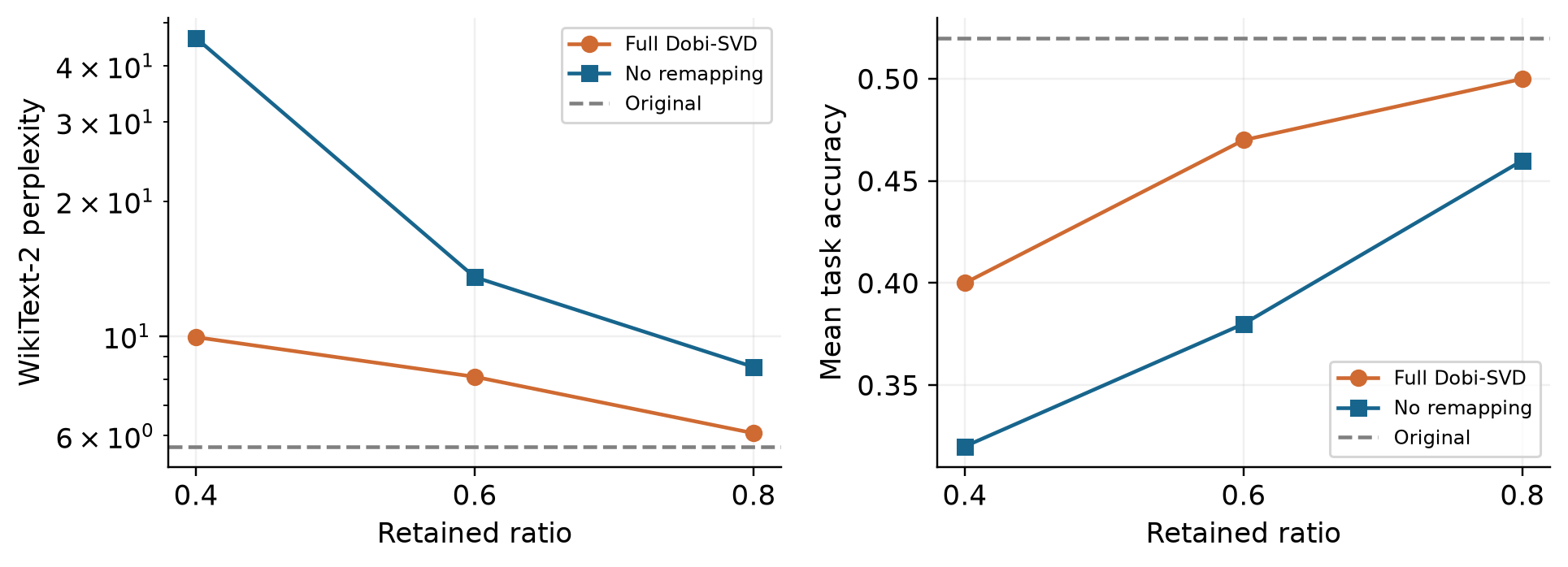
Figure 7. Replotted values from Table 2 of arXiv:2502.02723v1. The gain from the combined representation is substantial, while the gap to the uncompressed model remains visible at aggressive budgets.

The paper’s abstract and introduction report 9.07 for the 0.4 WikiText-2 configuration. Section 4.1 says 9.70. Table 2 and the conclusion say 9.95. The nearby baseline numbers also differ between prose and table. I cannot reconcile those statements from the document alone. Consequently, the plot and table here consistently use Table 2, and the discrepancy remains explicit rather than being silently averaged or corrected.

8.2 Rank learning helps, but not on every reported corpus

Table 16 isolates rank learning without remapping by comparing a uniform cutoff with the learned cutoff. At ratio 0.4, WikiText-2 PPL improves from 58.02 to 46.18, and PTB improves from 270.16 to 238.91. But C4 worsens from 145.41 to 190.62. This is a particularly informative exception to the accompanying statement that the learned ranks consistently improve performance across datasets.

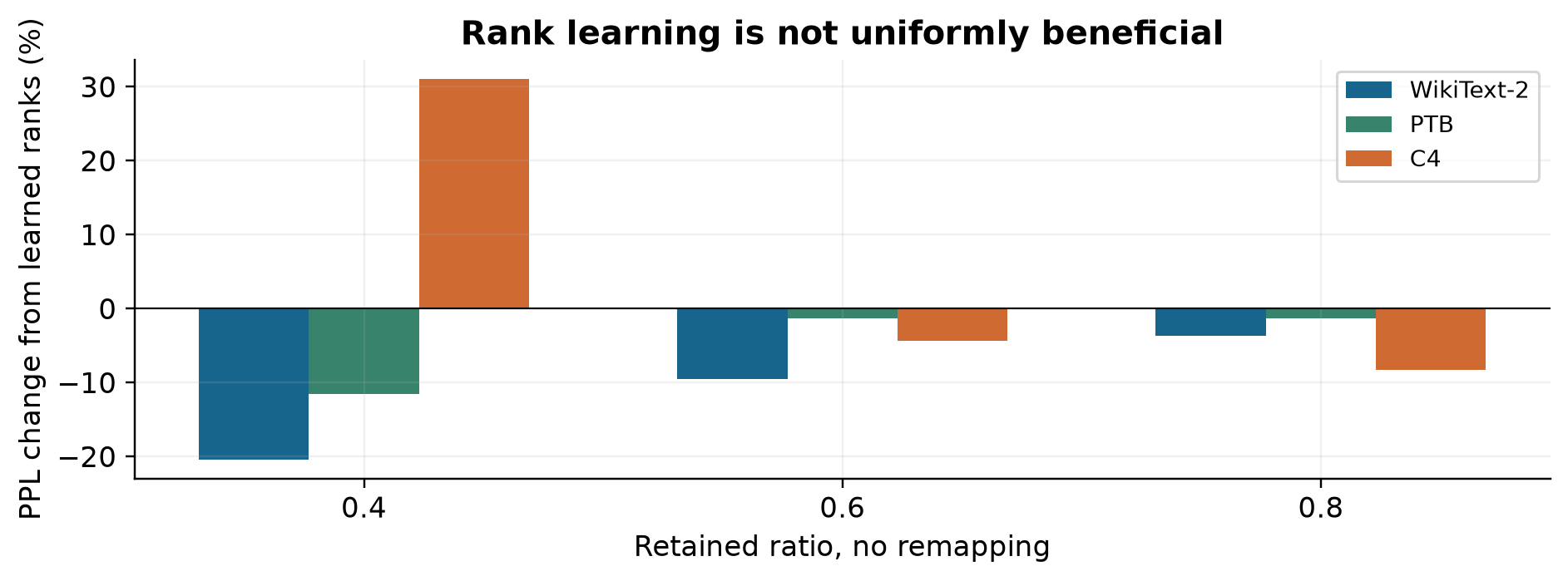
Figure 8. Relative PPL change from learning ranks, using Table 16. Negative values are improvements. At retained ratio 0.4, C4 changes in the opposite direction from WikiText-2 and PTB.

That pattern is compatible with an optimization process favoring its calibration distribution. It does not by itself prove overfitting, because the paper does not isolate all possible causes. It does mean that task-guided allocation should be evaluated on data outside the source of its gradients. A method that learns only a few hundred parameters can still specialize a powerful model’s bottlenecks to a narrow calibration objective.

The remapping ablation in Table 8 also distinguishes full-precision factors at the remapped rank from the mixed-precision version. At 0.4, their WikiText-2 PPL values are 9.78 and 9.95. This supports a modest quantization cost at that particular rank. Comparing that pair is different from comparing full Dobi to a lower-rank, equal-storage method. One isolates precision loss; the other changes both retained rank and precision.

8.3 More demanding tasks expose a different boundary

Table 6 reports MMLU for LLaMA-2-7B and LLaMA-3.1-8B. The original scores are 41.0 and 63.3. At retained ratio 0.8 they become 38.6 and 60.1; at 0.6, 27.5 and 50.1; and at 0.4, 24.1 and 28.2. In particular, LLaMA-3.1-8B loses 35.1 points at the most aggressive setting. Strong results against other compression baselines do not erase that absolute capability loss.

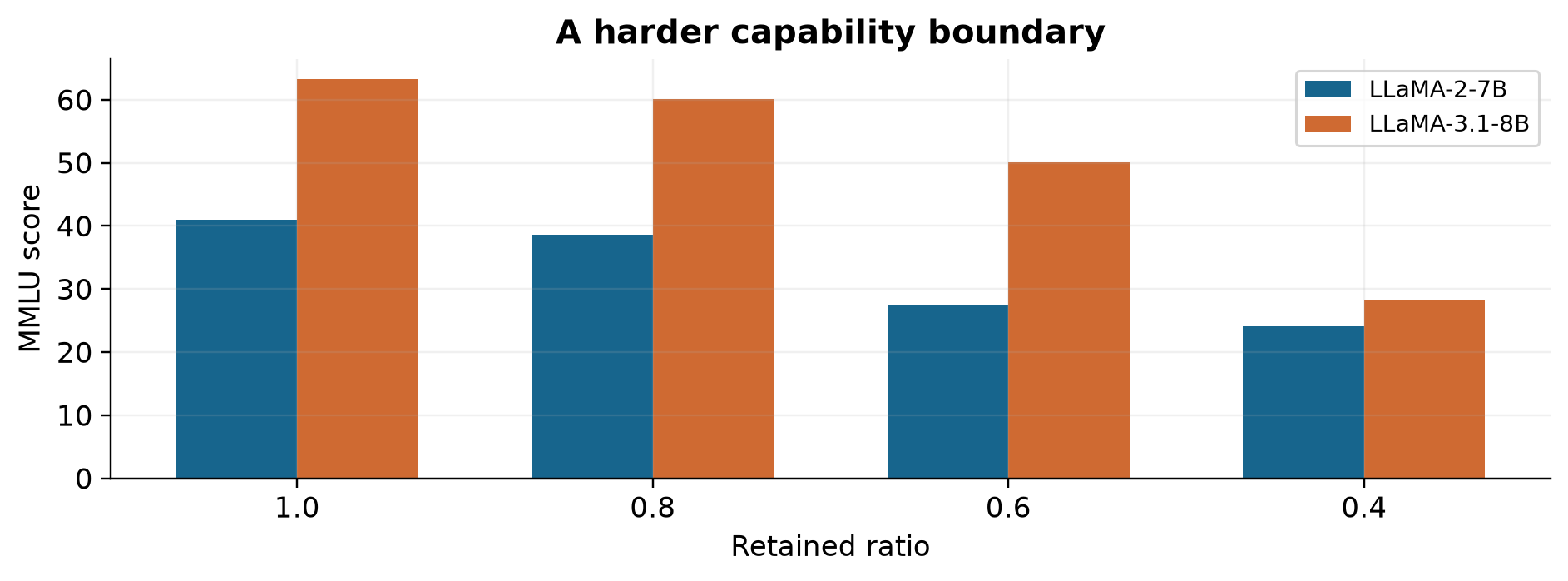
Figure 9. Reported MMLU scores from Table 6. The quality threshold for a deployment can be much stricter than the threshold suggested by a single perplexity measure.

The appendix extends the evaluation to 13B models and gives examples of generated text. Those examples help show that the models can produce language after compression, but a few hand-selected responses do not estimate a generation success rate. They cannot establish preservation of long-form coherence, tool-use reliability, or factual accuracy over a task distribution. The relevant follow-up is broader generation evaluation with an explicit sampling protocol.

9. The speedup depends on which memory boundary is crossed

9.1 The Titan Xp result is partly a residency transition

Table 10 reports 2.09 tokens/s for the original model and 25.97 tokens/s at retained ratio 0.4 on a 12GB Titan Xp. Their ratio is approximately 12.4. The text explains that the original model requires CPU–GPU transfers, whereas the compressed model fits on the GPU. This is valuable practical evidence, but it compares two memory-residency regimes.

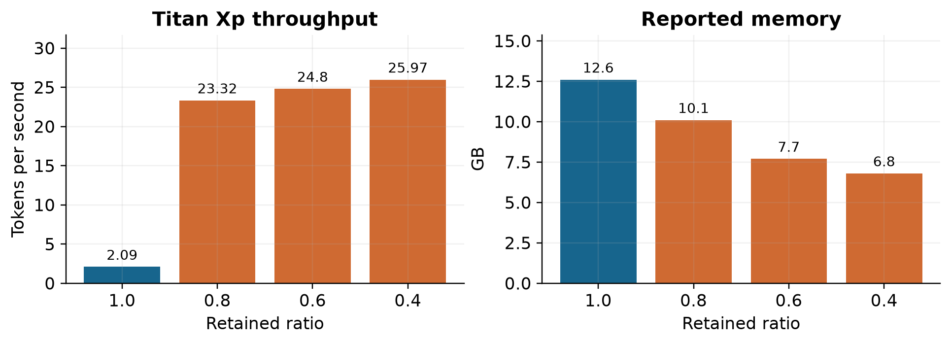
Figure 10. Table 10’s reported throughput and memory figures. The large speedup includes avoiding CPU–GPU movement; it should not be read as a twelvefold arithmetic improvement on a fully resident dense model.

A simple latency decomposition helps explain the result:

$$T_{\mathrm{token}}=T_{\mathrm{compute}}+T_{\mathrm{weight\ movement}} +T_{\mathrm{conversion}}+T_{\mathrm{other}}. \tag{16}$$

Compression can reduce the second term discontinuously when all relevant weights begin fitting in device memory. The first term may change more gradually, while mixed precision can add conversion work. The equation is an accounting model, not a timing model fitted to the paper. It shows why the same representation may produce very different speedups on two GPUs.

There is another reporting boundary: the text mentions roughly 14.8GB for the original model, while Table 10 lists 12.6GB in its original-model memory row. Without a matching definition of each memory figure, the exact peak allocation should not be inferred from either number alone. The qualitative offloading explanation is explicitly stated, but a precise capacity analysis would require a consistent accounting of weights, runtime buffers, and caches.

9.2 Fully resident performance is a separate experiment

The paper’s Figure 4 evaluates an A100 and varies batch size and sequence length. Section 4.3 describes up to 1.75 times throughput at retained ratio 0.4 and up to 1.4 times at 0.6 for that experiment. These are much more moderate than the Titan Xp ratio. The distinction is expected: if the dense baseline is already resident, the compression no longer removes the same host-transfer bottleneck.

Throughput is also not interchangeable with per-request latency. Larger batches can improve matrix utilization while increasing waiting time; short decode contexts can emphasize weight costs, while longer contexts expose attention and KV-cache costs. A good deployment comparison would specify batch, prompt length, generated length, precision, and memory placement together. Without those conditions, one headline speedup cannot be transported to an unrelated serving workload.

The paper also reports combinations with GPTQ and bitsandbytes. Table 9’s 0.6 Dobi-plus-GPTQ point is 2.4GB and PPL 9.97, whereas other sections contain different size descriptions. The safe reading is to cite a complete row from a named table. Table 23 uses a particular Hugging Face/bitsandbytes comparison and explicitly discusses avoiding kernel-optimized quantization baselines. It therefore cannot establish a universal runtime ranking against every optimized quantized deployment.

10. Multimodal extension and design alternatives

The multimodal experiments compress the language component of LLaVA-v1.5 and OpenVLA. This is a reasonable transfer test because large linear maps remain a major part of those systems. It is still a transfer of one component, rather than a demonstration that every vision encoder, action head, or cross-modal interface tolerates the same compression rule.

For LLaVA at retained ratio 0.4, Table 11 gives POPE-random accuracy 89.8 versus 88.1 for the original, but Science QA falls from 70.22 to 52.38 and TextQA from 58.22 to 46.72. The reported task-average row is not fully consistent with an arithmetic average of its displayed entries, so I rely on individual task columns here. A favorable hallucination-related score should not conceal the much larger changes on other tasks. Table 12 reports 20.1% throughput improvement at batch 16 for this setting, which is a useful system-level observation with its own quality cost.

OpenVLA’s Table 13 reports coordinate and angle mean squared error and a binary-action accuracy, alongside throughput. At ratio 0.4, accuracy is 0.9297 compared with 0.9570, and angle MSE is 0.3132 compared with 0.2929. These are offline action-prediction metrics. They do not establish a 92.97% closed-loop robot task success rate. A small mean error can hide occasional large errors, and a rollout can compound errors over time. The reported increase from 3.97 to 4.67 tasks/s is about 17.6%, but the meaning of “task” in the timing unit must remain tied to that evaluation.

Several alternative design choices help locate Dobi-SVD’s contribution:

Choice	Why it can be attractive	Main limitation
Weight SVD	Simple, data-independent factorization	Ignores input geometry
Input-whitened reconstruction	Directly models activation error	Conditioning and distribution mismatch
Differentiable rank allocation	Uses end-to-end task feedback	Repeated decomposition and backward cost
Discrete rank search	Avoids SVD derivatives	Candidate-evaluation cost and search resolution
Mixed-precision low-rank factors	Trades precision for retained directions	Quantization error and runtime handling
Dense quantization	Preserves full matrix rank	Hardware and low-bit error constraints

These choices can be combined. The useful comparison is not a categorical contest between “SVD” and “quantization.” It is whether a particular rank, bit-width, and execution arrangement achieves a better quality–memory–latency point. Dobi-SVD makes the joint nature of that decision especially visible.

11. Limitations and failure boundaries

Calibration is both a computational cost and a statistical assumption. The learned boundaries and recovered subspaces depend on sampled data. A coding assistant, multilingual model, or long-context agent may use directions that are weakly represented in WikiText-2. The C4 exception in Table 16 makes this concern concrete without proving a single cause. Calibration diversity and a held-out task distribution matter even when only rank controls are trained.

Shared-subspace recovery introduces approximation beyond local truncation. A basis derived separately for each batch carries input-specific structure. Replacing these with one basis changes the problem; streaming truncation may change it again. A fixed-rank reconstruction theorem should therefore be scoped to the exact objective and data used in its derivation. The aggregate objective is not a harmless implementation detail.

The bit budget is idealized. Quantization scales, padding, alignment, uncompressed embeddings, temporary buffers, and KV caches can all make whole-model memory differ from the factor-only ratio. Likewise, retaining a larger rank can increase arithmetic. A compressed checkpoint, a resident model, and an end-to-end serving process have different memory footprints.

Numerical stability is not exact differentiability everywhere. Finite-series stabilization changes the backward signal near repeated singular values. Small-value thresholds add scale dependence. This may be a sensible numerical strategy, but it should be judged by stable optimization and final quality, not described as removing the underlying nonuniqueness of singular vectors.

The source contains unresolved numerical and exposition inconsistencies. Besides the headline perplexity discrepancy, the tables and prose differ on several ablation and comparison claims. The appendix’s training-curve axis and its listed epoch count also need care when interpreted together. These issues limit precision of comparison, even though they do not negate every reported result. I preserve the table identity for every numerical conclusion rather than construct a unified result that the source does not supply.

The experiments do not settle all deployment regimes. Most named base models are 7B–13B-scale families. The evaluated task distributions, hardware, runtimes, and contexts are specific. The multimodal action metrics are not closed-loop task success, and qualitative generations are not a generation benchmark. The measured points justify investigation of the method within these boundaries.

12. Independent critical analysis

12.1 The most valuable contribution is the decomposition of decisions

I find the paper most useful as a way to separate three decisions often collapsed into “choose a compression ratio.” First choose which activation directions matter; then choose how much of each layer’s spectrum to retain; finally decide how accurately to store the retained factors. Each decision has a different objective and cost. This framing is portable even if a later method replaces the particular gate, the incremental subspace estimate, or the quantizer.

The remapping result also helps explain why comparisons among low-rank methods can be misleading. At a fixed nominal ratio, one method may carry more directions in fewer bits, while another carries fewer directions in full precision. A quality gap can then come from the representation budget rather than a better subspace optimizer. A meaningful ablation needs both equal-rank comparisons and equal-byte comparisons; neither can substitute for the other.

12.2 The theorem chain needs narrower claims

Equation (2) is exact and useful. Equation (10) exactly characterizes an unweighted projector surrogate. The step connecting those two objectives to a global task-optimal compressed model is not established by the same algebra. In particular, minimizing an upper bound does not generally identify the minimizer of the bounded objective. The distinction should be part of the main explanation rather than hidden behind a broad “theoretically optimal” label.

The model-level discussion in Appendix A.10 similarly uses a first-order loss expansion and supporting experiments. For an activation perturbation $\Delta A$, the local expansion and its magnitude bound are

$$\Delta\mathcal L\approx\langle G,\Delta A\rangle, \qquad |\langle G,\Delta A\rangle| \le\|G\|_F\|\Delta A\|_F, \quad G=\frac{\partial\mathcal L}{\partial A}. \tag{17}$$

A smaller norm reduces an upper bound; it does not order the actual inner products. For example, a unit error parallel to a loss gradient can have greater first-order effect than a larger error perpendicular to that gradient. This elementary fact prevents a general task-loss ordering from being deduced solely from the EYM theorem. The sampled-layer experiments provide empirical support in their setting, not a proof for all activations and models.

12.3 The strongest practical gain and the fairest comparison

Fitting entirely in GPU memory can matter more to a user than a modest improvement in theoretical operations. Dobi-SVD’s Titan Xp result is valuable for that reason. But a fair deployment decision also includes a dense quantized model, a smaller native model, and other representations that fit in the same memory. The paper explores several of these comparisons; it does not establish a universal winner across their quality and hardware combinations.

Table 24 is a useful example of a tradeoff that its surrounding prose overstates. The compressed LLaMA-13B row has higher mean accuracy than the original 7B row, 0.54 versus 0.51, but lower throughput: 38.6 versus 42.3 tokens/s at batch one, and 283.2 versus 319.5 at batch eight. That is a quality–speed tradeoff, not simultaneous dominance. Table 25 compares different model families and finds a different outcome; it should not be generalized into an architecture-independent rule.

12.4 What evidence would most reduce uncertainty?

Three targeted studies would be especially informative. The first would compare the learned ranks under held-out generation tasks, so that improvements in calibration perplexity can be separated from preservation of behavior. The second would compare exact aggregate subspaces, streaming approximations, and input-weighted recovery at a fixed rank, isolating the cost of the shared-weight bridge. The third would report matched end-to-end byte and latency measurements with and without remapping, including metadata and temporary memory.

These are proposals for interpreting or extending the research, not experiments performed for this review. Their value is that each changes one uncertain link in the argument. Broadly adding more benchmark rows would be less decisive if the representation budget, calibration objective, and runtime regime were still mixed together.

13. Conclusion

Dobi-SVD shows why low-rank compression is a joint geometry, allocation, and representation problem. Its activation-to-weight identity gives an exact answer for one calibration matrix. Differentiable cutoffs allow layer budgets to respond to task loss. Mixed-precision factors make additional rank affordable. Together these ideas yield strong reported quality relative to several low-rank baselines, and large practical gains when compression removes offloading.

The conditions around those results are essential. Shared recovery is a surrogate problem; stabilized SVD gradients are approximate near degeneracy; smaller stored factors do not always mean fewer operations; and strong perplexity comparisons do not establish preservation of every capability. Keeping those distinctions explicit makes the paper more useful: we can reuse its ideas without inheriting claims that its mathematics or experiments do not fully support.

References and reading scope

1. Qinsi Wang, Jinghan Ke, Masayoshi Tomizuka, Yiran Chen, Kurt Keutzer, Chenfeng Xu. Dobi-SVD: Differentiable SVD for LLM Compression and Some New Perspectives. Version 1, 2025-02-04. This review uses the 30-page PDF, including Appendices A.1–A.10, and the author list attached to that arXiv version.
2. Dobi-SVD author project page. Resource locator for the paper and its associated materials.
3. Official Dobi-SVD resource entry. Linked as a resource for interested readers.

Equations (1)–(17) use consistent dimensions and provide explanatory derivations, with the specific source approximations identified in the text. Figures 1–6 are original analytical illustrations; Figures 7–10 replot explicitly cited table entries. No new language-model training, benchmark measurement, or reproduction result is claimed.