M*: What a Multimodal Serving Runtime Must Know About the Model

Review date: 2026-10-15
Paper reviewed: M*: A Modular, Extensible, Serving System for Multimodal Models
Paper authors: Atindra Jha, Naomi Sagan, Keisuke Kamahori, Irmak Sivgin, Rohan Sanda, Steven Gao, Mark Horowitz, Luke Zettlemoyer, Olivia Hsu, Jure Leskovec, Baris Kasikci, Stephanie Wang
Identifier and version: arXiv:2606.12688v2, revised 2026-06-13; first submitted 2026-06-10
Resources: Paper and appendices · Official resource entry

1. The problem is the execution structure

A text generation server can often organize its entire life around two operations: process a prompt, then repeatedly generate a token. A modern multimodal model can require several distinct loops inside one request. An image-editing request may encode an image, prefill a transformer, run multiple guidance branches at every flow step, combine their results, and decode a final latent image. A speech request can instead stream hidden states from one transformer to another while an audio decoder consumes partial chunks. The shared requirement is execution over heterogeneous components, with dependencies that change by task.

M* asks what the serving runtime must see to optimize this structure. Its answer is a Walk Graph: a model graph, a set of named walks through that graph, and a state machine that selects the next walk for each request. Physical placement is specified separately. This exposes composition without requiring the scheduler to know what an image or a waveform means. The scheduler still needs precise information about dependencies, state, iteration boundaries, and streaming readiness. These are the pieces of model semantics that make generic execution possible.

The strongest contribution is the boundary between the model and the serving system. A model author describes components and execution structure. A deployer maps those components to devices. A runtime supplies batching, caching, graph replay, scheduling, and transport. The paper then shows that this separation can preserve useful optimizations across several model families. It does not establish that arbitrary future models require no integration effort, or that one placement is optimal for every workload.

This review reads the 20-page v2 paper, including its appendices. Reproduced figures are attributed to Jha et al. under the paper’s CC BY 4.0 license. The equations and algorithms labeled as explanatory below are my analytical reconstructions; they are not additional experiments or verbatim algorithms from the paper. Reported measurements refer to the authors’ experiments. The distinction matters because much of this paper is a systems abstraction, and its implications are broader than the particular speedups shown in the plots.

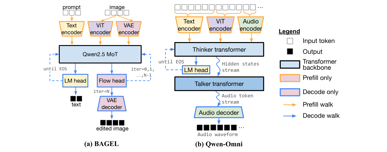
Figure 1. Original paper Figure 1, cropped from page 3. BAGEL and Qwen-Omni contain different loops and streaming dependencies; a single autoregressive token loop cannot describe both at the right scheduling granularity. Source: Jha et al., arXiv:2606.12688v2, CC BY 4.0.

2. Prerequisites: graphs, state, and serving metrics

2.1 A model graph is not a device schedule

A computation graph describes which tensors must exist before an operation can run. It does not necessarily say where an operation runs, which other request shares its device, or whether an intermediate tensor should be transferred. The same logical graph can be executed on one GPU, split across several GPUs, or partly replicated. Keeping these concerns separate is necessary if deployments are to change without rewriting the model’s control flow.

In M*, a node is a model component evaluated at a useful forward-pass granularity. A whole diffusion engine can hide dozens of iterations inside one stage. Exposing one iteration as a graph-level operation allows the runtime to schedule around its boundary. Conversely, exposing every arithmetic instruction would create too much scheduling overhead. The paper chooses a component-level boundary between these extremes. This is an architectural choice, not a proof that finer granularity always helps.

A graph with a loop is also different from a directed acyclic graph, or DAG. One can unroll a bounded loop into a large DAG, but doing so duplicates the description and obscures the state shared across iterations. Dynamic stopping, such as reaching an end-of-sequence token, is more naturally represented as an explicit loop with a termination rule. The runtime must distinguish the current iteration from the next even when both use the same node names.

2.2 What can be reused between calls?

Autoregressive attention reuses keys and values for an unchanged prefix. A paged KV cache manages those stored tensors in blocks, reducing allocation waste and allowing requests to grow independently. It does not make every intermediate activation reusable. A changing image latent can invalidate state that depends on that latent; an unchanged conditioning prefix may still be reusable. The dependency structure, rather than the model’s modality label, determines whether caching is valid.

CUDA graph replay addresses a different cost. It records a GPU execution sequence and replays it with compatible shapes and storage. It can reduce repeated launch overhead. It neither creates missing model parallelism nor automatically handles arbitrary shape changes. Continuous batching is different again: requests can enter or leave a batch at iteration boundaries, avoiding the need to wait for every request to finish a complete sequence. M* combines these mechanisms, but their benefits should not be attributed to a single primitive.

2.3 Keep the units straight

For text, time to first token measures the delay before useful output begins, while throughput measures output or requests completed over time. For image generation, end-to-end latency is often the most direct user-facing quantity. For speech, the paper uses real-time factor, RTF, and audio throughput. These are related but not interchangeable:

$$\mathrm{RTF}_i=\frac{T_i^{\mathrm{processing}}}{D_i^{\mathrm{audio}}},\qquad Q_{\mathrm{audio}}=\frac{\sum_i D_i^{\mathrm{audio}}}{T_{\mathrm{window}}}. \tag{1}$$

An RTF below one means a request’s overall processing time is shorter than its generated audio duration. It does not guarantee smooth playback: the first chunk might arrive late, or later chunks might have gaps. A useful streaming evaluation also considers first-audio latency and the distribution of chunk arrival deadlines. Likewise, median RTF cannot simply be inverted to obtain aggregate audio throughput under concurrent execution.

3. The Walk Graph contract

The paper declares a model as a pair consisting of a directed graph and a finite set of named walks. A walk represents a phase of a request, such as text prefill, image prefill, autoregressive decoding, or image generation. A model-provided state machine selects the next walk based on the request and the result of the current phase. The runtime is responsible for executing that choice.

An explanatory formalization separates three mappings:

$$G=(N,E),\quad \mathcal W=\{w_1,\ldots,w_m\},\quad \delta(r,w,o)=w_{\mathrm{next}}. \tag{2}$$ $$\pi(n,w)\subseteq\mathcal R. \tag{3}$$

Here $\delta$ is the request’s transition rule, $o$ denotes a completed walk’s outputs, and $\pi$ maps a node, optionally conditioned on its walk, to GPU ranks in $\mathcal R$. The first expression is logical behavior; the second is physical deployment. This notation helps explain the paper rather than specifying a complete executable interface.

There are four composition primitives. Sequential connects sections in a chain. Parallel permits children to execute concurrently. Loop repeats a section a bounded number of times. DynamicLoop adds per-request early termination. GraphNode and GraphEdge are the atomic computation and tensor-connection types. A streaming edge adds an input-buffer policy; it is not a fifth composition primitive in the paper’s four-primitive taxonomy.

Two details are easy to miss. First, Parallel means that dependencies allow concurrency. If its branches share one constrained GPU, physical overlap can be limited or absent. Second, Loop distinguishes terminal output from accumulated output. A terminal channel delivers the final iteration’s tensor; an accumulated channel retains contributions across iterations and emits the concatenation. Confusing them can produce both incorrect results and very different memory costs. Appendix B explicitly makes the channel names disjoint.

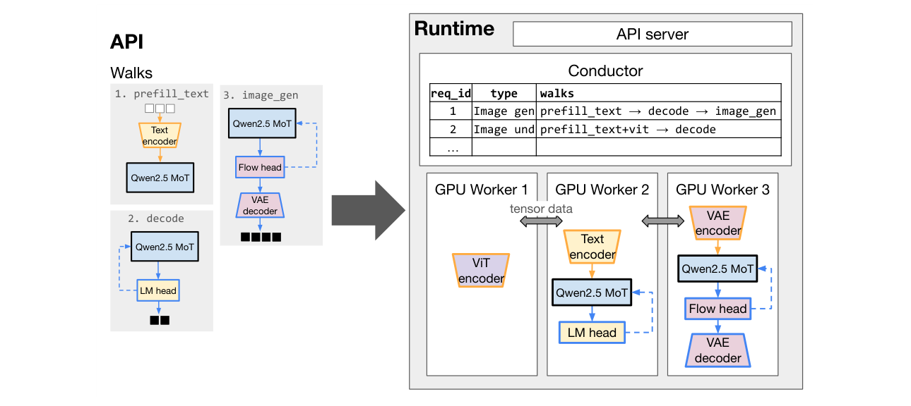
Figure 2. Original paper Figure 2, page 4. Model walks are defined on the left; device placement and execution live on the right. The drawing illustrates the abstraction and should not be read as the exact placement of every benchmark. Source: Jha et al., CC BY 4.0.

Algorithm 1. Dependency-driven execution of a request

The following numbered pseudocode reconstructs the semantics described in Sections 3.1–3.3. It abstracts away transport protocols, memory ownership, and failure recovery.

01  Choose the request's initial named walk using its input modalities.
02  Initialize per-request node inputs, loop state, and stream buffers.
03  Until the request is complete:
04      Find nodes whose required inputs and chunk policy are ready.
05      Map ready nodes to workers using placement(node, walk).
06      Combine compatible ready work into engine batches.
07      Execute a batch; associate each output with its request/iteration.
08      Route tensors to successors or append them to stream buffers.
09      At a loop boundary, retain or accumulate outputs as declared.
10      Advance the loop, or exit when its bound/stop condition is met.
11      When a walk ends, ask the model state machine for the next walk.
12      Emit terminal outputs and release state that is no longer needed.

The key correctness condition is that a ready node receives the inputs belonging to the same logical request and iteration. A producer finishing is insufficient if a consumer needs several branches or an entire chunk. Similarly, completion of one walk does not imply that all request state should be freed: another walk may reuse the same cached prefix. The graph contract reduces model-specific scheduling code by making these boundaries explicit, not by removing the need for them.

4. BAGEL: exposing a loop and its internal parallel branches

BAGEL is a useful example because one transformer backbone participates in several tasks. Image understanding eventually produces text. Image generation iterates a latent state. Image editing also conditions on an input image. M* describes these as different walks over shared components instead of forcing all requests through one fixed chain.

For guided image generation, the paper’s Appendix F expresses a loop whose body contains parallel transformer branches followed by a combine operation. The combine operation performs the guidance combination and an Euler update. The updated latent returns to the branches; only after the final iteration does the VAE decoder produce an image. The listing uses 49 Euler updates, described as num_timesteps - 1, while the experiment uses a 50-step flow schedule. These refer to the schedule grid and its update intervals; they should not be silently rewritten as 49 versus 50 identical forward operations.

Let $v_b$ be a branch output and $a_b$ a configured guidance coefficient. An explanatory generic linear combination and Euler step can be written as:

$$v_{\mathrm{guided}}=\sum_{b=1}^{B}a_b v_b,\qquad z_{k+1}=z_k+\Delta t_k\,v_{\mathrm{guided}}(z_k,t_k). \tag{4}$$

This is deliberately a schematic relation, not the complete BAGEL guidance formula. The evaluated setup also mentions guidance renormalization. Exact coefficients and renormalization must remain model-specific. What the runtime needs is the fan-out, the join dependency, and the loop-carried state. It can preserve those relationships while the combine component owns the actual numerical rule.

The critical-path benefit of branching has a simple conditional bound. Suppose the branches take $t_1,\ldots,t_B$, the join and update take $u$, and communication and scheduling add $c$. For a serial branch execution and an ideal concurrent execution:

$$T_{\mathrm{serial}}=\sum_{b=1}^{B}t_b+u,\qquad T_{\mathrm{parallel}}\geq\max_b t_b+u+c. \tag{5}$$

Subtracting the second expression from the first gives the largest available time saving under these assumptions. Parallel placement is useful only when the saved branch time exceeds the extra coordination cost. An imbalanced branch limits the gain even with unlimited bandwidth. Adding ranks can also duplicate weights and conditioning state, so lower latency need not imply lower GPU-seconds per image.

Algorithm 2. Guided image-generation walk

01  Prepare the conditioning state and initial latent z.
02  For each scheduled Euler update k:
03      Fan out z and time index k to the guidance branches.
04      Run each branch using its own conditioning context.
05      Wait until the required branch outputs are all available.
06      Apply the model's guidance combination and renormalization.
07      Compute the Euler update and carry the new latent into step k+1.
08  Decode the final latent through the VAE decoder.
09  Emit the image; reclaim loop state after downstream use finishes.

The paper also changes cache handling: guidance contexts are labels over one paged KV pool instead of separate dense, model-specific caches. A label is an additional cache identity axis, not an assertion that distinct conditioning contexts have identical keys and values. The optimization removes avoidable tensor concatenation and gives each context access to paging and related runtime mechanisms. This is a concrete reason a good abstraction can improve performance: it makes established optimizations applicable in a place where ad hoc state management previously hid them.

5. Streaming edges turn arrival into a scheduling decision

Speech generation makes the difference between an edge and a streaming edge concrete. A Talker may consume one hidden-state item as soon as a Thinker produces it. An audio decoder may need a group of codec frames, possibly with preceding context, before it can generate the next waveform segment. Triggering both consumers with the same policy would impose unnecessary waiting or provide insufficient context.

The paper supplies three policies. FixedChunkPolicy fires every $K$ items. SlidingWindowChunkPolicy waits for $W$ items and then advances by stride $S$. LeftContextChunkPolicy prepends $L$ older frames to a chunk containing $C$ new frames. These policies determine readiness and reuse at the edge, while the consumer still owns the semantics of the computation. Qwen3-Omni uses a fixed size of one on the Thinker-to-Talker edge and left-context chunking on the Talker-to-Code2Wav edge.

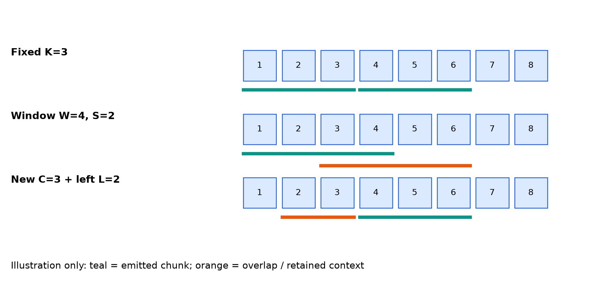
Figure 3. Explanatory diagram by Zhongzhu Zhou. Fixed chunks, overlapping windows, and retained left context make different promises about which items a consumer receives. The illustrated values are examples, not the paper’s benchmark settings.

For a fixed chunk size $K$ and $n$ produced items, the number of complete chunks is $\lfloor n/K\rfloor$. A residual fragment needs an explicit end-of-stream decision. The primitive description alone does not justify assuming that every incomplete final chunk is discarded, padded, or emitted unchanged. That behavior must follow the model’s valid input convention.

For a sliding window with positive $W$ and $S$, the number of complete windows is:

$$N_{\mathrm{windows}}(n)= \begin{cases} 0,&n<W,\\ 1+\left\lfloor\dfrac{n-W}{S}\right\rfloor,&n\geq W. \end{cases} \tag{6}$$

The derivation counts the first window after $W$ arrivals and then one additional window for every $S$ arrivals. When $S<W$, input is intentionally reused. Under a simple linear-cost consumer model, each new item participates in roughly $W/S$ processed positions over a long stream. This is useful context, but it is also redundant computation. The numerical cost model is explanatory and need not match an audio decoder’s nonlinear kernel behavior.

For left-context chunking, after startup, $C$ new frames can require processing $C+L$ input frames. The corresponding input-work amplification is:

$$A_{\mathrm{context}}\approx\frac{C+L}{C}=1+\frac{L}{C}. \tag{7}$$

Shrinking $C$ can reduce chunk-formation delay while increasing this overhead. If producer interarrival times are approximately constant at $\Delta$, the first full chunk waits about $(C-1)\Delta$ after the first new frame arrives, plus consumer queueing and service time. This exposes a latency-efficiency tradeoff that cannot be settled by a universal default chunk size.

Algorithm 3. Streaming readiness with retained context

01  Append each arrived frame to the buffer for this request and edge.
02  Ask the selected policy whether a valid consumer input is ready.
03  If ready, form its new-frame region and any retained context.
04  Dispatch only when other consumer dependencies are also satisfied.
05  Advance the logical stream position according to the policy.
06  Retain only frames needed by future windows or left context.
07  On producer completion, resolve the final fragment per model rules.
08  Finish the edge only after outstanding consumer work has completed.

Buffers create another obligation: bounded memory. If arrivals exceed consumption for a sustained period, the buffer grows even though every local computation is correct. With arrival rate $\lambda$ and service rate $\mu$, a simple fluid approximation gives a backlog change of $\lambda-\mu$ while the queue is nonempty. Stable operation needs adequate capacity or admission/backpressure controls. M* provides a structure in which such policies can be expressed; its reported results do not establish a complete overload-control design for every streaming application.

6. Placement: exposing choices does not choose them

M* allows a graph node to map to one or more GPU ranks, optionally differently across walks. This supports separating prefill from decode, replicating a component, or colocating components that exchange many small tensors. Tensor parallelism is specified at the node level, with model authors using provided sharded layer counterparts. It therefore still requires integration into the model; the deployment description alone does not transform arbitrary layers into a distributed implementation.

Consider two successive components. Splitting them across devices can overlap requests and allow independent scaling, but it adds a transfer cost. A rough transfer-time model is:

$$T_{\mathrm{transfer}}=\alpha+\frac{B_{\mathrm{tensor}}}{\beta}, \tag{8}$$

where $\alpha$ is fixed overhead, $B_{\mathrm{tensor}}$ is bytes transferred, and $\beta$ is effective bandwidth. A sequence of many tiny chunks can be dominated by $\alpha$ even when the total byte volume is small. Combining chunks can amortize that cost but increases waiting. Colocation removes a process or transport boundary yet causes the components to compete for one device’s compute and memory bandwidth.

The evaluated Qwen3-Omni configuration uses two H200s, with the Thinker on one GPU and Talker plus Code2Wav on the other. The important relationship is the colocation of the latter two components. The main text and appendix swap the numeric rank labels; the labels themselves do not alter that topology. The appendix’s generic three-partition example is a description of a possible graph placement, not the exact two-GPU experiment.

Physical feasibility also imposes a memory constraint. A practical plan must fit weights, live KV state, activations, stream buffers, and replay workspaces. Summing weights alone is insufficient. A useful deployment study would sweep the distribution of request types and lengths because that distribution changes the live state and the bottleneck. M* exposes the placement space; automatic search for a good placement is a separate problem, one reason Cornfigurator is a useful follow-up reading.

7. Runtime: hide planning without violating dependencies

The paper describes an HTTP entry point, a Conductor tracking request walks, and one worker process per GPU rank. Control work is dispatched through ZeroMQ, while tensors can move directly between workers. The data plane supports shared memory and Mooncake-based transports. The evaluation uses single-node shared-memory transport, so support for RDMA is a capability rather than a demonstrated cross-node speedup.

Workers host engines. The paper names KVCacheEngine for stateful transformer work and StatelessEngine for simpler nodes. Engines support batching, CUDA graph replay, and compilation. A local round-robin policy drives engines. Round-robin is understandable and relatively simple, but equal turns do not imply equal service time: a long image step can consume more device time than a short speech step. Fairness and deadline guarantees need their own analysis.

The runtime overlaps CPU preparation of batch $N+1$ with GPU execution of batch $N$. In particular, it double-buffers attention plans and prepares the next plan on a separate thread and CUDA stream. It alternates between anticipating readiness along the current walk and scheduling already-ready unrelated work. The purpose is to avoid leaving the GPU idle while the host constructs metadata.

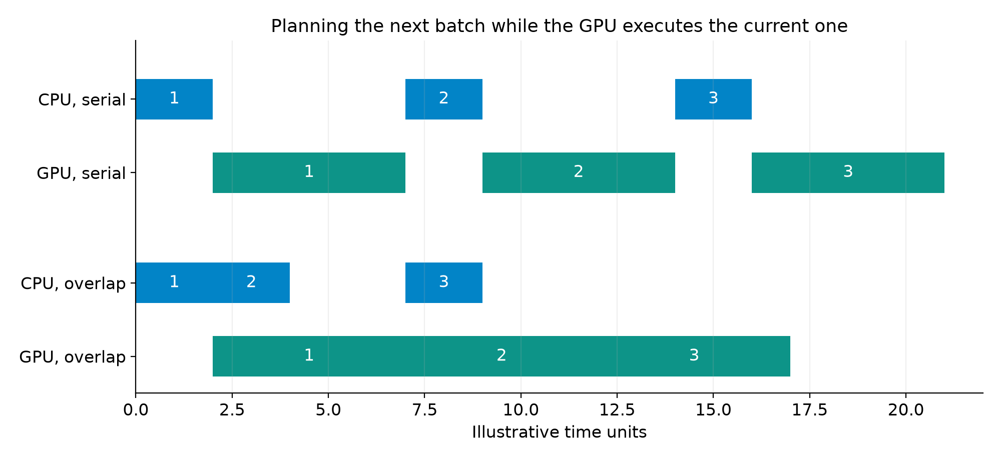
Figure 4. Explanatory timeline by Zhongzhu Zhou, using invented time units solely to illustrate overlap. Numbers identify batches. Planning batch 2 while batch 1 runs removes an idle interval; this picture is not a profiler trace from M*.

Let $c$ be CPU preparation time and $g$ GPU execution time for an idealized fixed-size batch. Without overlap, $N$ batches take $N(c+g)$. With perfect pipeline overlap and no extra contention, the first batch still pays both costs, and each additional batch advances at the slower stage’s rate:

$$T_{\mathrm{serial}}(N)=N(c+g),\qquad T_{\mathrm{pipe}}(N)=c+g+(N-1)\max(c,g). \tag{9}$$

Dividing and taking the large-$N$ limit gives:

$$S_{\infty}=\frac{c+g}{\max(c,g)}\leq2. \tag{10}$$

This bound applies only to hiding these two serial stages. It does not bound the whole system’s speedup, which may additionally eliminate redundant work or improve kernels. Conversely, it warns against attributing a very large gain solely to CPU-GPU overlap. A system already dominated by GPU compute has little host planning time to hide.

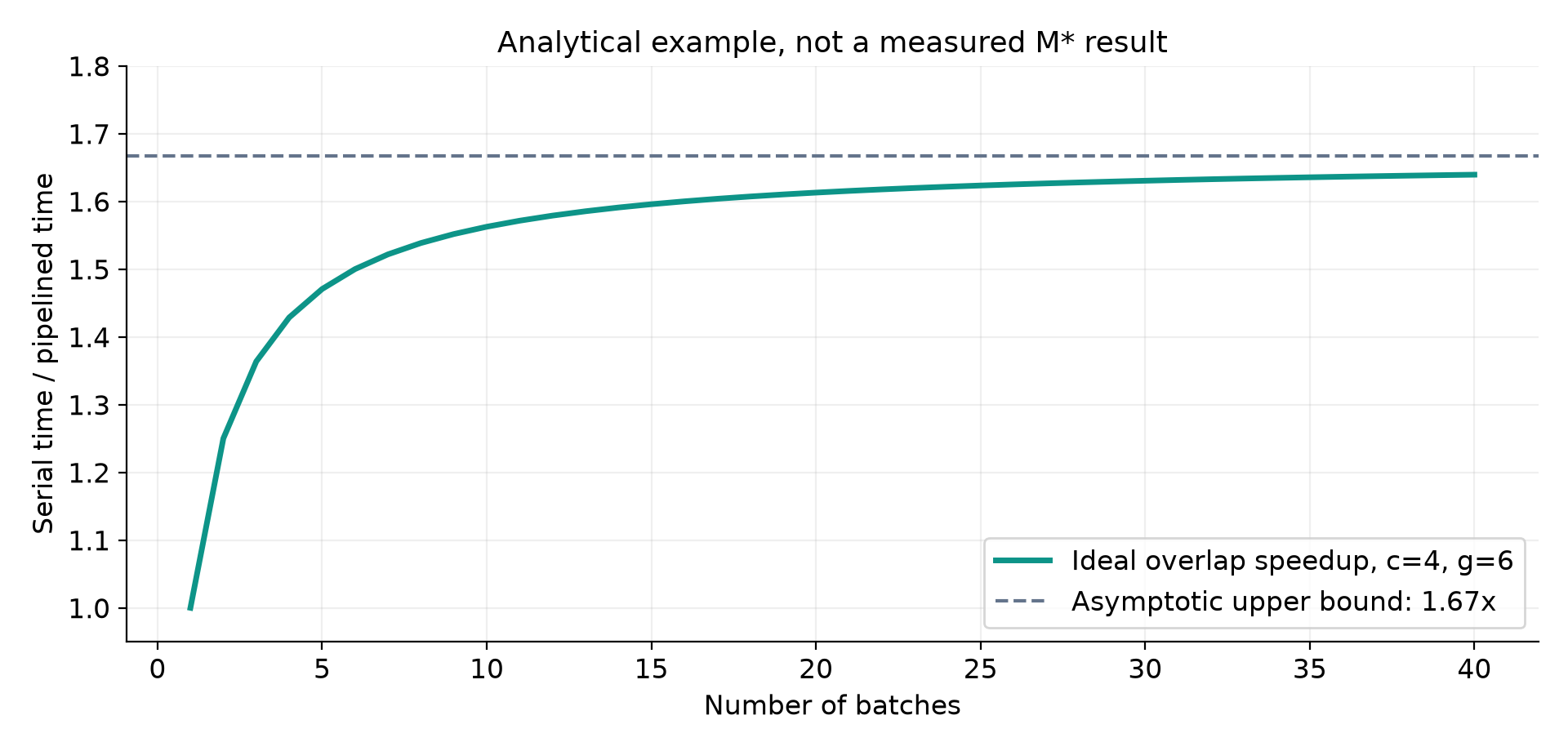
Figure 5. Analytical illustration by Zhongzhu Zhou. For $c=4$ and $g=6$ arbitrary time units, ideal overlap approaches $10/6\approx1.67$ times speedup. Startup costs reduce the gain for short runs. These values are not measured results.

DynamicLoop creates a subtler problem: the next iteration may be prepared before the current iteration reveals that the request should stop. The paper defers the termination check to the next boundary, allowing at most one wasted step per termination, and allows speculation to be disabled per node. This is execution scheduling speculation, not speculative token acceptance. It should not cause an extra output to be exposed to the client.

A simple expected-cost argument makes the tradeoff explicit. If speculation hides host work $h$ per scheduled boundary, termination probability is $p$, and the extra step costs $g_{\mathrm{extra}}$, then a rough local benefit condition is $h>p g_{\mathrm{extra}}$, ignoring resource contention. For a long-running loop, termination is rare over most boundaries. For a short or expensive action loop, the wasted step can dominate. If an operation has externally visible side effects, computing an unwanted extra action may be inadmissible even when its arithmetic cost is small. The paper’s disable option is therefore semantically important.

8. BAGEL results: the baseline configuration matters

The BAGEL experiments cover text-to-image generation, image editing, and image-to-text understanding. Generation uses a 1024-scale image output and a 50-step flow schedule. The three-GPU configuration assigns one H100 to each guidance branch; the image-understanding experiment uses one H100. This distinction prevents the image-generation and text-understanding results from being mistaken for one identical hardware setup.

The paper compares against two vLLM-Omni configurations. The default has separate Thinker and diffusion stages, while the single-stage version avoids that boundary. For image editing, transferring state between the default stages is particularly costly. M* can reuse one underlying component and preserve its efficient cache path across the walks. The single-stage baseline removes a substantial part of this penalty, so it is the more informative comparison for isolating the remaining latency gap.

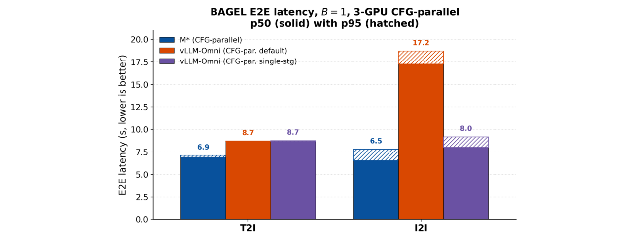
Figure 6. Original paper Figure 3, page 8. Batch size 1, three H100s, guidance branches parallelized. Solid bars represent p50 and hatched extensions p95. Source: Jha et al., CC BY 4.0.

For T2I the plotted p50 labels are approximately 6.9 seconds for M* and 8.7 seconds for either baseline configuration. For image editing they are approximately 6.5 seconds for M*, 17.2 for the default baseline, and 8.0 for the single-stage baseline. The paper reports speedup ratios of 1.25 and 1.22 against the single-stage baseline, and 2.64 for image editing against the default. Small differences when recomputing from plotted labels are expected because the labels are rounded.

A ratio and a reduction percentage use different denominators:

$$S=\frac{T_{\mathrm{base}}}{T_{\mathrm{new}}},\qquad R=\frac{T_{\mathrm{base}}-T_{\mathrm{new}}}{T_{\mathrm{base}}} =1-\frac1S. \tag{11}$$

Thus 1.25 times speedup means a 20% latency reduction, not a 25% reduction. A 2.64 times ratio corresponds to roughly 62% lower latency, but against the more expensive default pipeline. Reporting only the largest ratio would hide the stronger single-stage baseline and overstate how much of the gain survives after that baseline’s obvious transfer bottleneck is removed.

For image understanding, the main experiment fixes output lengths by ignoring EOS, with lengths uniformly distributed from 64 to 256. At batch size 16 the paper reports 32.7% higher throughput and 25.5% lower per-request end-to-end latency. The controlled length helps separate serving efficiency from output-length differences, but it also removes natural stopping behavior. Conclusions about real conversations with varying stop times require additional measurements.

The single-GPU image-generation appendix is useful because it shows gains without distributing guidance branches: it reports a 1.13 times T2I ratio and image-editing ratios of 1.66 against the default and 1.25 against the single-stage configuration. This supports the claim that cache management and execution organization matter independently of branch placement. It does not provide a complete ablation isolating every optimization.

9. Qwen3-Omni and Orpheus: speech is a pipeline

9.1 Qwen3-Omni’s two-GPU experiment

Qwen3-Omni has a Thinker producing text and hidden states, a Talker producing codec tokens, and Code2Wav converting them to audio. The two-GPU experiment places the Thinker on one H200 and the latter two components together on another. It uses Seed-TTS. This is a natural case for combining a fine-grained graph with component-level engine optimization.

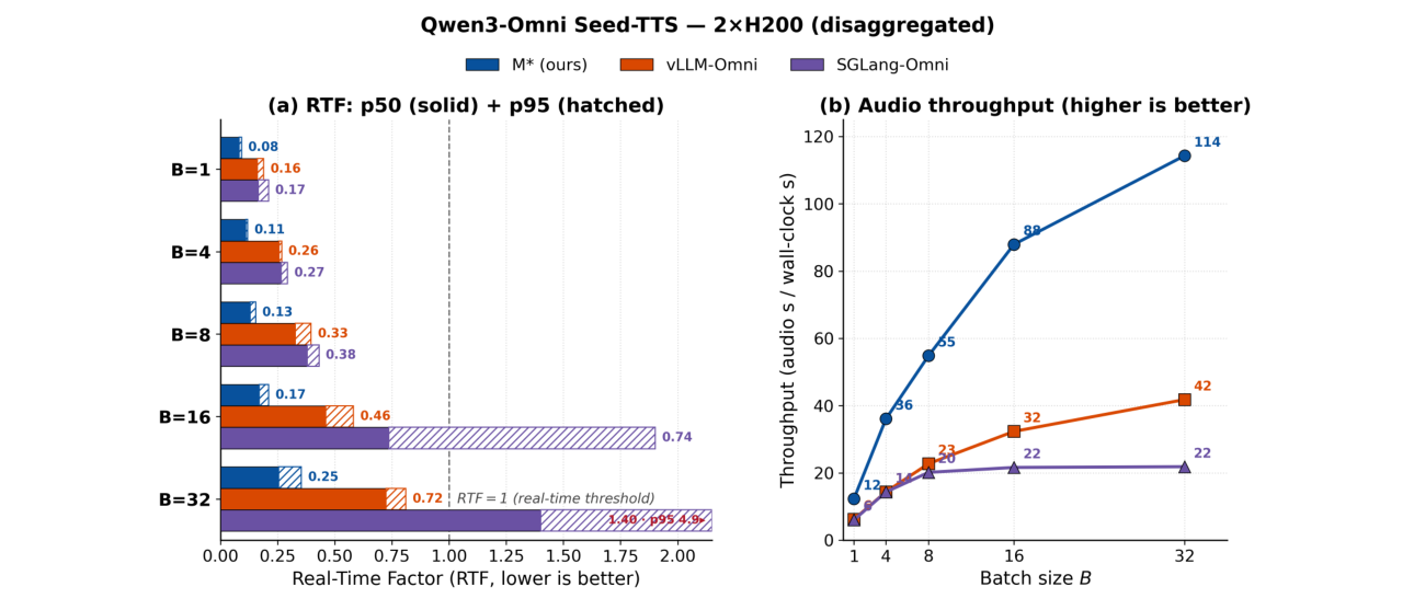
Figure 7. Original paper Figure 5, page 9. Two H200s, Seed-TTS, RTF on the left and generated-audio seconds per wall-clock second on the right. Read the axes carefully: audio throughput is neither tokens per second nor requests per second. Source: Jha et al., CC BY 4.0.

At batch size 16 the paper reports approximately 2.7 times audio throughput relative to vLLM-Omni and 4.0 times relative to SGLang-Omni. Its mechanism explanation has two parts. First, per-submodule capture lets the Talker, including its multi-token predictor loop, run as a CUDA graph. Second, placing Talker and Code2Wav in the same worker avoids a cross-process boundary for their small streamed tensors. These are specific runtime choices enabled by modular composition; the primitive names themselves do not accelerate a kernel.

At batch size 32 the plot labels show audio throughput of about 114, 42, and 22 audio seconds per wall-clock second for M*, vLLM-Omni, and SGLang-Omni respectively. Those values should not be relabeled as the batch-16 result. Similarly, the largest RTF advantage in an abstract need not occur at the same batch size as a selected throughput comparison.

The paper also reports Thinker tensor parallelism of degree two, using three H200s overall, against SGLang-Omni. It states that the corresponding vLLM-Omni configuration could not be made to work. The missing result is missing evidence, not a zero-throughput competitor. The measured comparison is narrower than a claim that M* dominates every baseline at every parallel configuration.

9.2 Orpheus exposes a reporting discrepancy

Orpheus-3B is compared with the speech-focused VoxServe on a single H200 and Seed-TTS, averaged over five trials. The graph includes a language model streaming into an SNAC audio decoder. The paper attributes gains to reusable model-level optimizations and asynchronous attention planning. This is a useful test of whether a general runtime can compete with a domain-specific system.

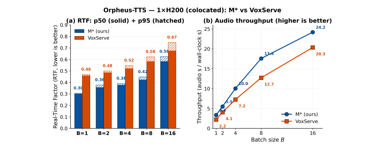
Figure 8. Original paper Figure 7, page 10. The throughput panel labels approximately 24.2 and 20.1 at batch size 16, which imply about a 20% gain. This differs from the introduction’s 39% claim at that batch size. Source: Jha et al., CC BY 4.0.

The RTF claim of 13.6% lower median at batch size 16 is consistent with the rounded plotted values, about 0.58 versus 0.67. The throughput reporting is less consistent. The introduction says 39% higher at batch size 16; the graph’s 24.2 versus 20.1 implies about 20%. At batch size 8 the graph shows about 17.5 versus 12.7, which implies about 38%, while Section 4.3 says 20% at batch size 8. The batch labels or the textual percentages appear mismatched. The paper alone does not resolve which description is intended.

For that reason, this review uses the graph’s displayed values when doing arithmetic and explicitly preserves the discrepancy. It does not silently exchange batch labels or claim a corrected experimental result. The safe conclusion is that the plotted configuration favors M* across the shown batch sizes, with a gain whose exact textual summary needs clarification. The paper’s appendix also lists an Orpheus placement split over two ranks while the main experiment and figure say one H200; the figure should be interpreted as the reported one-GPU comparison, without assuming that the appendix listing is its exact configuration.

10. V-JEPA 2: a large gain from avoiding repeated prefix work

The world-model experiment compares action-conditioned rollouts against the native V-JEPA 2 baseline on one H100, batch size one, with horizons 4, 15, and 30. Inputs come from the first 50 DROID episodes. M* expresses the rollout as a DynamicLoop and reuses keys and values across steps. The baseline, as described by the paper, repeatedly processes a growing prefix without KV caching.

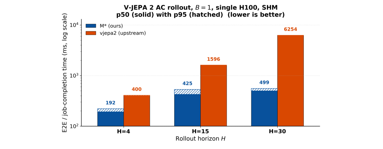
Figure 9. Original paper Figure 8, page 11. The vertical axis is logarithmic. Rounded p50 labels are 192 versus 400 ms at horizon 4, 425 versus 1596 ms at horizon 15, and 499 versus 6254 ms at horizon 30. Source: Jha et al., CC BY 4.0.

The authors report ratios of 2.08, 3.76, and 12.5 at the three horizons. The growing advantage is consistent with removing repeated work, but the plot is not proof that M* has invented a new attention algorithm. It demonstrates that a world-model loop can use an established state-management optimization through a reusable serving engine.

An explanatory count shows why horizon matters. Suppose a prefix begins with $P$ token-equivalents and every rollout step adds one. If the baseline recomputes the full prefix’s projection work at step $h$, then the total projected positions are:

$$W_{\mathrm{repeat}}=\sum_{h=1}^{H}(P+h) =HP+\frac{H(H+1)}2. \tag{12}$$

If cached prefix states remain valid, the corresponding position count becomes roughly $P+H$: one initial prefix plus one newly appended position per step. This is a count of reusable projection work, not total attention FLOPs. Each new query still attends to the growing cache. For full causal attention recomputed at each step, summing quadratic prefix costs can grow cubically in $H$; cached incremental attention instead sums linearly growing query-to-cache costs, giving a quadratic contribution. Neither simplification predicts the measured speedup by itself.

The assumptions are decisive. A world-model update that changes previous states, applies bidirectional attention to the entire evolving sequence, or changes masking in a way that alters old keys and values may invalidate the cache. Cached inference must preserve the model’s mathematical dependencies. The useful systems lesson is to ask which state is invariant across iterations and expose that fact to the runtime.

For attribution, a stronger baseline would add KV caching and comparable batching to the native rollout while retaining its simpler serving structure. The remaining difference would help isolate generic runtime overhead and optimization portability. The reported 12.5 times result is valuable as an end-to-end improvement over the stated baseline, but it cannot be assigned entirely to Walk Graph scheduling.

11. Design alternatives and their operating boundaries

A fixed stage pipeline remains attractive when a model’s execution pattern is stable and each stage already has a strong optimized engine. Fewer exposed scheduling boundaries can reduce overhead and simplify reasoning. It becomes restrictive when loops span stages, different request types take different paths, or a shared component should remain live across multiple walks.

A monolithic per-model engine can optimize aggressively across the entire request. It can fuse operations and avoid generic dispatch. Its cost is repeated engineering as architectures change, especially when each model invents its own cache and streaming conventions. M* offers a middle ground: model-specific numerical components inside a common execution contract. The contract is useful only when component interfaces are precise enough to preserve state and dependency semantics.

A record-and-replay approach can recover task dependencies from a more imperative model program. That may ease adoption for existing code. M* instead asks authors to declare structure ahead of time, making loops and component boundaries visible earlier. This trades explicit integration work for runtime knowledge. The paper discusses Cornserve in this comparison, but its reference number points to an arXiv entry now titled Cornfigurator; these names should not be treated as interchangeable descriptions of an unchanged artifact.

Three deployment choices illustrate the limits:

Choice	Why it can help	When it can lose
Split components across GPUs	Independent scaling and overlap	Small chunks or large state transfers dominate
Colocate Talker and codec	Avoid process-boundary overhead	Device contention or memory pressure increases
Expose loop iterations	Reuse batching and scheduling	Very short kernels make dispatch cost significant
Use larger stream chunks	Amortize invocation and transport	First output and playback deadlines worsen
Speculate next-iteration planning	Hide host work	Frequent stopping causes expensive wasted work

These are conditional tradeoffs. A graph representation makes the choices available and comprehensible. It does not supply a universal cost model, an admission policy, or an optimizer that always picks the best combination.

12. Limitations and unresolved evidence

The evaluation covers several model families, but quantitative results are shown for four: BAGEL, Qwen3-Omni, Orpheus, and V-JEPA 2. The paper also describes support for $\pi_{0.5}$ without presenting a separate benchmark for it. Support is therefore broader than the measured performance evidence. It would be misleading to claim that all five families received the same depth of empirical testing.

All reported experiments use single-node hardware with shared-memory tensor transport and intra-node NVLink. A runtime may support RDMA while still lacking demonstrated multi-node efficiency. Inter-node latency, bandwidth contention, transport scheduling, failure recovery, and replicated state introduce additional costs. The paper’s flexible placement API should be read as enabling such deployments, not validating them.

The current engines and streaming policies cover the evaluated models. Appendix H explicitly leaves other engines, chunk policies, sequence/context/pipeline parallelism, more advanced asynchronous scheduling, and further modality-specific optimizations for future exploration. An extensible interface is an investment in future support; it is not evidence that an untested integration will be effortless or fast.

The benchmark protocol also contains inconsistencies. Section 4 says 5–10 warmup requests; Appendix I says 3–5 and lists a default of three. Appendix E’s Figure 10 caption says output lengths 16–128, while its nearby prose says 16–64. The Orpheus placement and throughput discrepancies were discussed above. These issues do not erase the measured trends, but they limit how precisely a reader can reconstruct the intended setup from the text alone.

The experiments mostly use offline waves with specified concurrency. Such tests are useful for capacity comparisons, but they do not establish behavior under bursty arrivals, mixed image/audio/text requests, cancellations, or overload. Sharing a component across walks is a capability; robust isolation between those walks requires evidence about tail latency and resource contention. Output-quality equivalence is another necessary axis: forced greedy settings and length controls reduce some variation, but a broad quality comparison across image, audio, and robotics outputs is not established by latency plots alone.

13. Critical analysis: separate expressiveness from causality

13.1 What the paper supports most strongly

M* gives a persuasive example of an abstraction that carries useful optimization information. Loops, branch joins, stateful components, and stream readiness are visible to a common runtime. A set of real composite models can be expressed through that interface and achieves favorable performance against the evaluated alternatives. This supports the engineering value of sharing runtime mechanisms across modalities.

The evidence for reduced developer effort is less complete. A concise graph listing is encouraging, but integration also includes numerical components, weight loading, sharding, sampling, shape constraints, and lifecycle behavior. The paper does not present a controlled study of implementation time or maintenance cost. “Day-zero support” should be treated as the design motivation, not an empirically guaranteed onboarding time.

13.2 Why the largest ratio is not the whole story

The experiments combine changes at several levels: graph abstraction, cache design, CUDA graph coverage, component colocation, attention planning, and baseline configuration. The system-level gains are real claims under the reported conditions, but causal attribution is underdetermined without matched ablations. The V-JEPA result is especially clear: removing repeated prefix work can produce a large gain even without proving that the scheduler is independently better.

A useful conceptual decomposition is:

$$T=T_{\mathrm{useful}}+T_{\mathrm{redundant}}+T_{\mathrm{launch}} +T_{\mathrm{plan}}+T_{\mathrm{transfer}}+T_{\mathrm{queue}}. \tag{13}$$

This is an accounting model, not an exact additive profiler model when terms overlap. Cache reuse reduces redundant work; graph replay reduces launch overhead; asynchronous preparation hides planning; colocation reduces some transfers. Queueing can increase while another term decreases. A convincing attribution study measures which components change rather than assigning every improvement to the abstraction’s name.

13.3 The next decisive experiments

The first useful comparison is a matched-optimization baseline: equal caching semantics, similar graph-capture coverage, and equivalent placement. If M* remains competitive, the result would quantify the cost of generality while retaining the abstraction’s integration advantage. The second is a mixed-workload test where one shared backbone handles text and image requests while speech has deadlines. The objective should be goodput under explicit service targets, not just average throughput.

The third is a placement sweep under the same total GPU budget. Include both latency and GPU-seconds per completed request, memory high-water marks, and transfer volume. A fourth study should report first-audio latency and deadline misses in addition to RTF. Finally, a multi-node test would distinguish transport support from practical performance once data leaves a fast intra-node fabric. These are proposed research evaluations, not experiments carried out for this review.

The most productive reading is therefore neither to dismiss the paper as a wrapper around known optimizations nor to credit a graph API for every speedup. The abstraction makes known optimizations reusable in more places. That is a substantial systems contribution when interfaces are precise and the runtime remains efficient. The remaining question is how much of that benefit persists as models, workloads, and hardware move beyond the benchmark envelope.

14. Conclusion

M* shows why a multimodal server should understand more than prefill and decode. Named walks, structured loops, parallel branches, streaming policies, and separate placement make a model’s execution structure available to reusable runtime machinery. The strongest measured examples arise when that machinery removes redundant state work or exposes an optimization that a coarser stage boundary concealed.

For a systems reader, the durable lesson is to choose an abstraction that exposes the dependencies an optimizer needs while preserving the numerical semantics the model owns. The benchmarks offer promising evidence across image, speech, and world-model workloads. Their scope remains single-node and configuration-dependent, with several reporting inconsistencies that should be resolved before using precise ratios as deployment forecasts.

References and figure sources

1. Atindra Jha et al. M*: A Modular, Extensible, Serving System for Multimodal Models, v2. Sections 2–4 provide the model, runtime, and experiments; Appendices A–I provide semantics, additional plots, and limitations. Original Figures 1, 2, 3, 5, 7, and 8 are reproduced with attribution under CC BY 4.0.
2. Keisuke Kamahori et al. VoxServe: Streaming-Centric Serving System for Speech Language Models. Follow-up reading on streaming-specific serving objectives.
3. Jeff J. Ma et al. Cornfigurator: Automated Planning for Any-to-Any Multimodal Model Serving. Follow-up reading on choosing deployment plans; this is the current title of the identifier cited under an older Cornserve title in M*.

The numbered explanatory algorithms, equations, and Figures 3–5 in this review are analytical teaching material by Zhongzhu Zhou. They introduce no new measured performance claims.