DART: Parallel Drafts, Local Continuity, and the Real Cost of Speculation

Review date: 2026-10-14
Paper reviewed: DART: Diffusion-Inspired Speculative Decoding for Fast LLM Inference
Paper authors: Fuliang Liu, Xue Li, Ketai Zhao, Yinxi Gao, Ziyan Zhou, Zhonghui Zhang, Zhibin Wang, Wanchun Dou, Sheng Zhong, Chen Tian
Identifier and version: arXiv:2601.19278v1, submitted 2026-01-27
Resources: Paper and appendices · Official resource entry

1. The question: when does the helper become the bottleneck?

Speculative decoding asks a cheap model to propose several tokens before an expensive model checks them together. It is tempting to judge the helper entirely by its accuracy: if it predicts more accepted tokens, fewer calls to the target should be necessary. DART starts from the other half of that bargain. A helper that makes eight small sequential predictions can still take enough time to erase the benefit of verifying them together. The useful objective is accepted progress per unit of elapsed time, including every stage required to produce that progress.

DART combines a single-layer, target-coupled neural drafter with an n-gram-guided tree search. The neural model predicts a short horizon of future-position distributions in one forward call. Those distributions are conditional on the known prefix, rather than on successively sampled draft tokens. A CPU-side n-gram model then helps rank locally compatible combinations before the target verifies the resulting tree. The target remains an autoregressive language model; the drafting process borrows masked parallel prediction from diffusion models without running an iterative diffusion sampler.

My main takeaway is that DART relocates dependency. It removes repeated neural forward calls from the drafter, then restores some cross-token consistency through an inexpensive discrete search. That is a plausible way to spend a latency budget, but it introduces a second resource budget: a large resident CPU index and the work needed to search it. Calling the neural layer lightweight does not make the entire serving configuration lightweight.

The paper’s central empirical result is convincing in its measured regime. Table 1 reports mean speedups of 2.42–2.87× for the Qwen3 family at temperature zero, compared with 2.01–2.20× for EAGLE3. At the same time, Appendix E shows that the advantage over ordinary decoding can nearly disappear at high batch size for Qwen3-8B. I therefore read this as a strong latency-oriented design with a meaningful operating region, rather than a universal replacement for all decoding workloads.

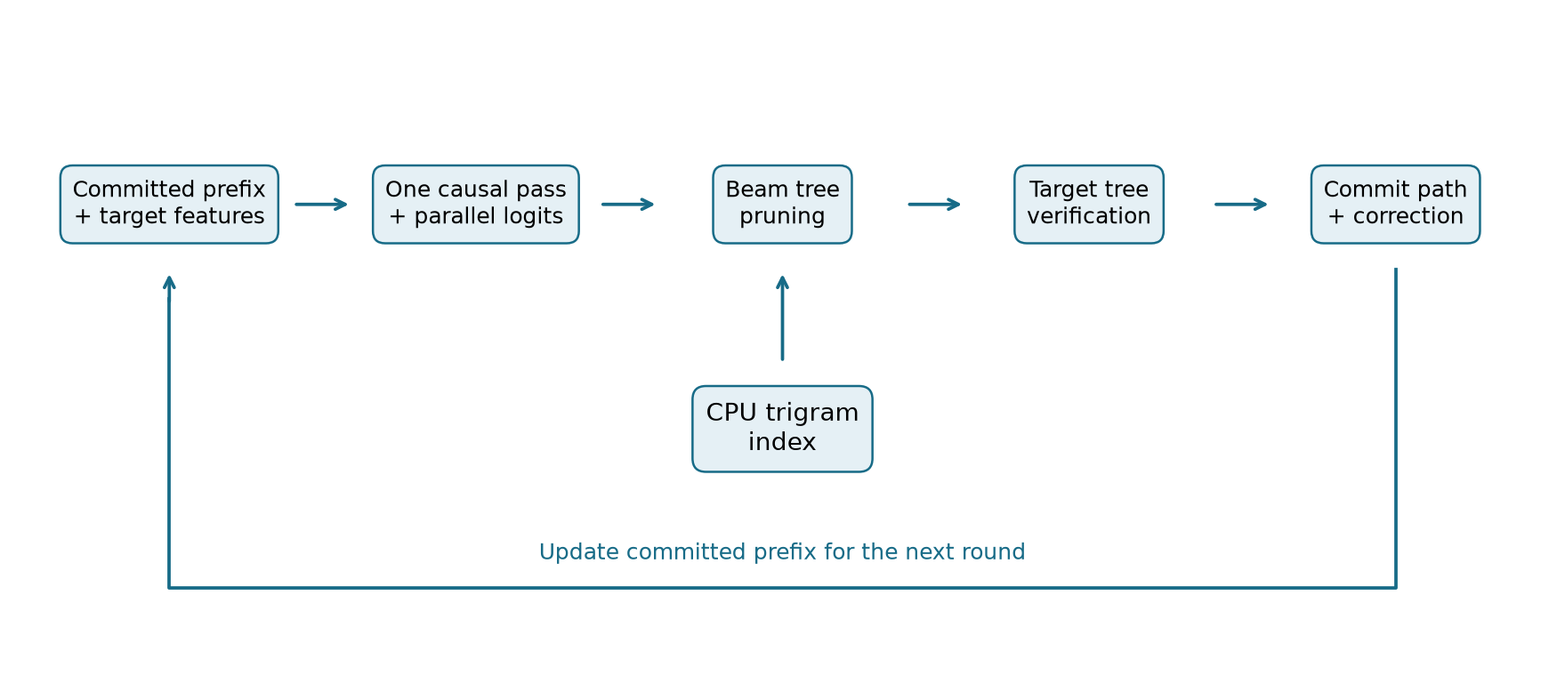
Figure 1. Original schematic based on paper Figure 3 and Sections 3–4. Target features feed a single parallel draft pass; local continuity enters during tree construction, and target verification determines committed output. The n-gram stage is a proposal filter, not the authority on output correctness.

2. Prerequisites: latency, accepted progress, and verification

2.1 A timing model that does not reward the wrong metric

Let $T_{\mathrm{AR}}$ be the time for one ordinary target-model decoding step. Let $T_D$, $T_S$, and $T_V$ denote draft forward time, search time, and target verification time per speculative round. Let $M$ be the number of tokens actually committed by that round, including any correction or bonus token under the chosen verifier. Ignoring prefill and fixed startup costs, the long-run speedup is approximately

$$S \approx \frac{\mathbb E[M]T_{\mathrm{AR}}}{\mathbb E[T_D+T_S+T_V]}. \tag{1}$$

This is a ratio of accumulated progress to accumulated time. It is not generally the mean of a per-round ratio. If hard requests simultaneously have low acceptance and high overhead, averaging each request’s speedup can conceal a different aggregate service-level outcome. The equation is a useful accounting model, not a replacement for an end-to-end measurement.

The paper uses $\tau$ for acceptance length, but its introductory definition emphasizes accepted draft tokens while the metrics paragraph describes tokens generated per cycle. That distinction matters when a verifier emits an extra token. I preserve the reported $\tau$ values and do not silently add one to them. For derivations below I use $A$ for accepted draft tokens and $M$ for committed tokens, so the convention stays explicit.

For a chain with $d$ proposals, let $a_i$ be the probability that position $i$ is accepted conditional on all earlier positions being accepted. The tail-sum identity gives

$$\mathbb E[A] =\sum_{i=1}^{d}\Pr(A\ge i) =\sum_{i=1}^{d}\prod_{j=1}^{i}a_j. \tag{2}$$

The conditional definition makes the product valid without assuming independent acceptance events. An error at the beginning prevents later correct proposals from helping. If all $a_i=a$, the expression reduces to $a(1-a^d)/(1-a)$ for $a\ne1$. This explains both the importance of early positions and diminishing returns from increasing the horizon.

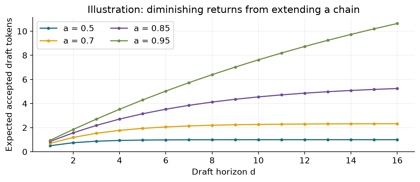
Figure 2. Original illustrative calculation from Equation (2), using constant conditional acceptance probabilities. These curves are not measurements from DART. Extending a weak chain adds little expected progress; improving early acceptance can matter more than a longer horizon.

2.2 Why a worse proposal need not change the target distribution

For ordinary single-token speculative sampling, write $q(v)$ for the target distribution and $p(v)$ for the actual proposal distribution. A proposal $v\sim p$ is accepted with probability $\min(1,q(v)/p(v))$. The accepted probability mass of token $v$ is therefore $\min(p(v),q(v))$. The total rejection probability is

$$R=1-\sum_v\min(p(v),q(v)) =\sum_v[q(v)-p(v)]_+. \tag{3}$$

If rejection occurs, sample from the normalized residual $r(v)=[q(v)-p(v)]_+/R$, when $R>0$. The unconditional mass becomes

$$\min(p(v),q(v))+Rr(v)=q(v). \tag{4}$$

When $R=0$, rejection never occurs and no residual needs to be formed. This elementary calculation explains the separation between proposal quality and output correctness. Poor proposals waste time; a correct acceptance-and-correction mechanism still produces the target distribution.

Equations (3)–(4) explain standard chain verification. They are not a proof of an unspecified tree sampler. DART constructs a ranked, pruned tree from factorized logits and n-gram scores; those scores are not automatically the proposal probabilities required by the equation. At temperature zero, comparing candidates with target argmax choices is straightforward. At positive temperature, the tree verifier must preserve the corresponding sampling invariant and fallback behavior. The paper states lossless generation but does not supply a detailed tree-verification derivation. That is a documentation limitation worth retaining in a technical reading.

3. Architecture: one neural pass does not mean one independent token

DART uses low-, middle-, and high-level hidden states extracted from the target after prefill or verification. Appendix B specifies the first, $(N/2-1)$-th, and $(N-4)$-th transformer layers for a target with $N$ layers, following the paper’s layer-number convention. A fully connected projection combines them into a compact representation. Shifted token embeddings provide information about the next token that the target has already sampled.

In the notation of Section 3.2, the feature construction can be summarized as

$$g_j=W_f[h_j^{\mathrm{low}};h_j^{\mathrm{mid}};h_j^{\mathrm{high}}]+b_f, \qquad z_j=[g_j;e_{j+1}]. \tag{5}$$

The paper writes an input $[z_{1:n},\mathrm{MASK}_{n+1:n+d-1}]$ and reads $d$ output logits: the first from the last prefix position, the rest from masked positions. Thus eight predictions require seven appended masks. This is a shifted prediction layout, not eight autoregressive invocations of a small model.

There is a subtle indexing issue here. The prose includes the already sampled next-token embedding while the training description uses a prefix-relative notation for predicting the next $d$ tokens. For understanding the design, the crucial invariant is which tokens are already known at each draft call. I would explicitly trace the known token, feature position, and prediction position when specifying a runtime integration, rather than infer an unmentioned off-by-one convention from the compact symbols alone.

The customized decoder has causal attention over the prefix and within the masked suffix. A later masked position can use earlier hidden representations in the same pass, but it does not receive an earlier newly sampled token and then trigger another forward call. Shared computation and causal hidden-state flow are compatible with parallel logits. They do not turn the outputs into a fully autoregressive joint distribution over candidate paths.

Why not use a full diffusion language model? A separate multi-billion-parameter denoiser can cost more per step than the lightweight target-coupled layer. Tokenizer compatibility and target-specific alignment also matter. DART instead gives up iterative refinement and limits the horizon, defaulting to $d=8$. The architectural tradeoff is fewer sequential calls at the price of less direct conditioning on the actual candidate sequence.

The paper describes drafting cost as independent of $d$ because there is one forward pass. I would qualify that statement: the number of sequential neural calls is constant, but the amount of attention and output-head work still changes with the number of positions. At sufficiently large $d$, neither GPU latency nor tree construction cost should be expected to remain constant. No broad horizon-scaling study is supplied to remove that caveat.

Algorithm 1. A conceptual inference round

This pseudocode explains the paper’s components; it is not an execution trace or an independently tested implementation.

1. Run target prefill, or retain the last target verification result.
2. Identify the committed prefix and the next target-sampled token.
3. Gather low/middle/high target features for the valid prefix.
4. Project their concatenation and pair it with shifted embeddings.
5. Append d - 1 learned mask representations with future positions.
6. Run the customized causal decoder once; obtain d logit vectors.
7. Build a compact candidate tree with Algorithm 3 below.
8. Verify that tree with target attention and a valid verifier.
9. Commit only the accepted path and required correction/bonus token.
10. Keep state for the committed prefix; discard rejected branches.
11. Repeat until a stopping condition or output limit is reached.

Step 10 is conceptually necessary even though DART avoids the repeated autoregressive draft rollout and its associated cache management. Target KV state, accepted-prefix alignment, and candidate-tree attention are still real responsibilities. Eliminating one category of cache complexity does not eliminate caching from speculative inference.

4. Training many prefixes without revealing their futures

4.1 The sparse mask is part of the learning problem

Training every prefix separately would repeatedly process the same clean tokens. DART instead shares one clean sequence across many masked training groups. Group $n$ sees clean prefix positions up to $n$ and its own causal masked positions, but no other group’s masked positions. Clean tokens use ordinary causal attention. Figure 3 illustrates that structure for a deliberately small example.

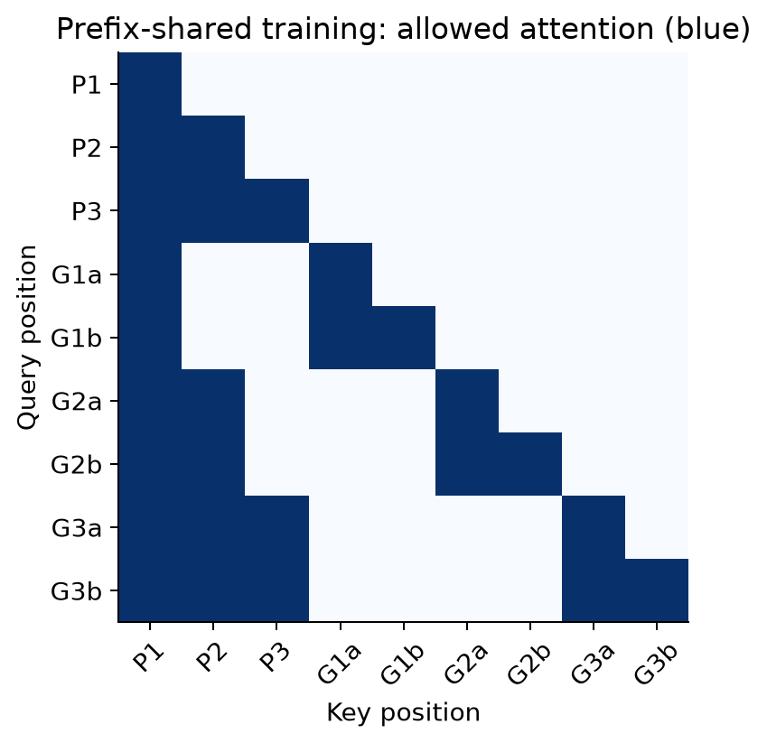
Figure 3. Original attention-mask illustration based on Section 3.3 and Appendix B. Blue cells are permitted attention. Three clean positions share separate two-mask groups. Each group has a different accessible prefix; masked groups cannot attend across groups. This toy uses a shorter horizon than the paper’s default.

The isolation rule prevents a particularly easy shortcut: a masked prediction for an early prefix must not read a clean future token elsewhere in the packed training sequence. Position IDs and attention eligibility are separate concepts. Reusing appropriate position IDs for different groups does not itself isolate their information; the explicit sparse mask does that. Conversely, a correct mask with incorrect relative positions can still train the wrong positional relationship.

Appendix B presents the mask as the union of three predicates: clean-query/clean-key causal access, draft-query/allowed-prefix access, and within-group causal access. FlexAttention exploits the resulting sparse structure. This improves execution efficiency while preserving the intended computation; the sparsity is not an approximation to unrestricted bidirectional attention. Dense attention with the same mask would define the same learning problem but could be much more expensive.

4.2 Why later targets are intrinsically harder

At future offset $t$, the target teacher distribution is conditioned on the true intervening tokens, whereas the drafter has only the initial prefix and position. Let $Y$ denote those intervening tokens, $x$ the known prefix, and $q_Y(v)$ the teacher’s next-token distribution. For a draft distribution $p(v\mid x,t)$, minimizing the expected forward KL gives

$$\begin{aligned} \mathbb E_Y[\mathrm{KL}(q_Y\Vert p)] &=C-\sum_v\mathbb E_Y[q_Y(v)]\log p(v),\\ \bar q(v)&=\mathbb E_Y[q_Y(v)],\qquad p^*(v)=\bar q(v). \end{aligned} \tag{6}$$

The constant $C$ is independent of $p$. Minimizing cross-entropy under the probability-simplex constraint yields $p^*=\bar q$. This is my derivation of what a prefix-only distribution learns under the stated objective, assuming sufficient model capacity and optimization. It is a mixture over possible intervening futures, not the teacher’s conditional distribution for every particular candidate branch.

That observation explains the need for structured pruning. A good marginal prediction at position three may combine outcomes that belong to incompatible futures. Making the marginal model larger can reduce modeling error, but it does not make all combinations of its marginal modes jointly plausible. The missing dependence must be represented somewhere else or resolved by target rejection.

4.3 Weighted KL and its gradient

The paper minimizes

$$\mathcal L=\sum_{t=1}^{d}\gamma^{t-1} \mathrm{KL}\!\left(q_\theta(\cdot\mid x_{1:n+t-1}) \Vert p_\phi(\cdot\mid x_{1:n},t)\right),\quad \gamma=0.6. \tag{7}$$

For one position, expand KL as $\sum_v q_v\log q_v-\sum_vq_v\log p_v$. The teacher is fixed, so its entropy contributes no draft-model gradient. With $p_v=\mathrm{softmax}(\ell)_v$, differentiating the weighted cross-entropy gives

$$\frac{\partial\mathcal L_t}{\partial\ell_v} =\gamma^{t-1}(p_v-q_v). \tag{8}$$

For eight positions, the weights are 1, 0.6, 0.36, 0.216, 0.1296, 0.07776, 0.046656, 0.0279936, summing to $2.4580096$. The first three positions receive about 79.74% of the total weight. These are direct calculations from the published coefficient, not learned importance scores. Scaling every weight by the same normalization would preserve the objective’s minimizer, although it would change gradient magnitude under a fixed optimizer configuration.

The term “annealed” here describes decay across future positions. The displayed objective does not define a changing $\gamma$ over training time. It should also not be confused with the cosine learning-rate schedule or the sampling temperature used for inference.

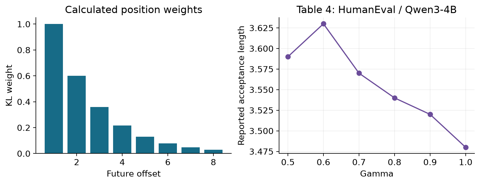
Figure 4. Left: weights calculated from Equation (7). Right: paper Table 4, HumanEval on Qwen3-4B. The measured acceptance length peaks at $\gamma=0.6$, but no uncertainty interval is reported. The weighting curve is mathematical; the acceptance curve is reported experimental data.

Algorithm 2. Prefix-shared training at the conceptual level

1. Obtain a clean training sequence and target teacher outputs.
2. Gather the selected target hidden states and shifted embeddings.
3. For each valid prefix, create its future masked prediction group.
4. Assign positions consistently with the corresponding draft horizon.
5. Allow causal attention among clean tokens.
6. Let each masked group see only its own prefix and causal group.
7. Run the lightweight draft layer with the sparse attention pattern.
8. Match each predicted offset to its teacher distribution.
9. Weight forward KL at offset t by gamma^(t - 1).
10. Mask padding/invalid targets, sum valid losses, and update drafter.

The last step states the usual validity requirement; the paper’s mask pseudocode explicitly tracks sequence validity. Exact normalization and sequence-boundary handling must be specified in a training recipe. The source does not justify replacing its teacher distribution with a one-hot label while retaining the same interpretation of Equation (7).

Appendix B reports approximately 280K filtered ShareGPT and UltraChat examples, context length 6400, three epochs, AdamW with learning rate $2\times10^{-5}$, gradient clipping 0.5, and optimizer betas $(0.9,0.999)$. The FC layer, decoder layer, LM head, and mask representation are trainable; the shared target embedding is frozen. Training uses eight H20-3e GPUs. A single-layer description therefore should not be mistaken for a complete parameter-count or training-cost comparison: the vocabulary head also contributes, and the paper does not provide a full budget-matched training study.

5. From marginal logits to a coherent candidate tree

5.1 A small counterexample to independent top choices

Imagine an illustrative two-position continuation with true probability 0.5 on “red apple” and 0.5 on “blue berry,” and zero on the two crossed combinations. Each marginal is perfectly predictable as a 50–50 distribution. Their product nevertheless allocates 0.25 to every pair, placing half of its mass on combinations that never occur. This toy is not a statement about actual language frequencies; it isolates the distinction between accurate marginals and an accurate joint distribution.

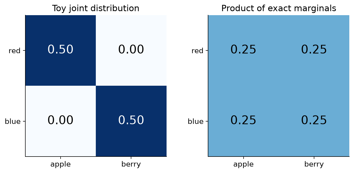
Figure 5. Original toy probability tables. The left table has strong cross-position dependence; multiplying its exact marginals produces the right table. DART uses short-context statistics to help rank candidate combinations, while the target provides the final check.

Selecting the single top token at every position would discard alternatives before the target can inspect them. Taking the full Cartesian product is also impractical. With $k=25$ candidates at each of $d=8$ positions, there are $25^8=152,587,890,625$ complete paths. Even a compact logit array can therefore imply an enormous verification workload.

DART keeps at most $w=20$ active partial paths at each depth and eventually selects at most $\theta=59$ tree nodes for verification. Under those default settings, an upper bound on candidate extensions scored during beam expansion is

$$N_{\mathrm{expand}}\le k+(d-1)wk =25+7\times20\times25=3525. \tag{9}$$

This counts expansions, not unique nodes after merging shared prefixes, and excludes logit top-$k$, sorting, and tree assembly costs. It explains the reduction in combinatorial work without pretending that the CPU stage is constant-time.

5.2 The ranking rule, interpreted carefully

Appendix D combines a draft log probability with an n-gram log probability. For depth $\ell$, a token extension receives the increment

$$\Delta s_\ell= \frac{0.9^{\ell}\log(p_\ell(v)+\epsilon) +0.5\log(g(v\mid c)+\epsilon)}{(\ell+1)^{0.7}}, \quad s_{\mathrm{new}}=s_{\mathrm{parent}}+\Delta s_\ell. \tag{10}$$

Here $g$ is the n-gram conditional score, $c$ is the recent candidate context, and $\epsilon$ is a numerical stabilizer. I retain the appendix’s depth symbol without resolving its zero-/one-based implementation convention. The logits become less trusted at larger depths through $0.9^{\ell}$; the n-gram term has fixed weight 0.5 before the shared depth factor. The depth factor reduces the magnitude of the negative penalty for later extensions.

Exponentiating a score increment reveals a useful interpretation:

$$\begin{aligned} \exp(\Delta s_\ell) &=(p_\ell(v)+\epsilon)^{0.9^{\ell}/(\ell+1)^{0.7}}\\ &\quad\times(g(v\mid c)+\epsilon)^{0.5/(\ell+1)^{0.7}}. \end{aligned} \tag{11}$$

It resembles a product of experts with depth-dependent exponents. Accumulated scores are ranking heuristics, not a calibrated probability distribution over complete trees. The search still needs to handle unseen contexts, smoothing, ties, and the budget for ancestor nodes. The paper does not fully specify every such corner case.

If each log probability is nonpositive, every extension lowers the cumulative score, so an ancestor scores at least as highly as its descendant. This helps explain why global top-node selection can retain prefix closure. The exact statement needs care with the added $\epsilon$: for a probability extremely close to one, $\log(p+\epsilon)$ can be positive. Ties also need an ancestor-safe policy. A practical tree specification should enforce ancestor closure explicitly instead of relying on an unstated score convention.

Algorithm 3. Continuity-aware pruning

This restates paper Algorithm 1 at the method level; the last line makes the verification-tree requirement explicit.

1. Set active paths C = {(prefix, score 0)} and global nodes T = {}.
2. For each future offset i from 1 to d:
3.     Select top-k_i tokens from parallel logit vector i.
4.     For every active path, retrieve its n-gram child scores.
5.     Extend the path with each candidate token.
6.     Add the combined score increment from Equation (10).
7.     Store the extensions in both temporary candidates and T.
8.     Retain the top-w extensions as the next active paths.
9. Select the top-theta scored nodes from T, as in the paper.
10. Represent the result with valid ancestors and tree attention.

The top-$k_i$ set is shared across active paths at the same future offset because the neural logits have not been recomputed for each path. The n-gram score is what changes with the candidate suffix. This is the precise location where path dependence re-enters. A trigram can favor locally compatible fragments; it cannot generally ensure long-range semantic or logical consistency.

6. The CPU index is an important part of the system

Appendix C reports a trigram trie built from Dolma 3 Mix with the relevant Qwen3 or LLaMA2 tokenizer. It contains about 1.3 billion nodes, occupies about 43.5 GB on disk, and uses roughly 100 GB of CPU RAM during inference. These are different measurements: serialized disk size is not resident memory usage. Dividing the reported RAM footprint by node count gives roughly 77 bytes per node using decimal units; this is only an aggregate estimate and does not reveal the data structure’s internal allocation layout.

For each active context, the trie traversal can locate the context node once and obtain scores for its candidate children. With the default beam parameters, there are at most $1+(d-1)w=141$ active contexts to query across a round. Multiplying that bound by the reported warm retrieval time of approximately 6 microseconds gives 0.846 ms of serial query service time. This is an illustrative calculation, not a prediction of complete search latency: top-$k$, score combination, parallelism, data movement, cache misses, and tree assembly also contribute.

The measured tree-search stage is about 2.0 ms in the Qwen3-14B example. The appendix describes CPU parallelism and binding the index and worker threads to the same NUMA node. These details explain why a per-query microbenchmark cannot be used as the whole runtime budget. An index that is warm and local on a server with 900 GB RAM need not behave the same way in a memory-constrained container or with many competing workers.

The paper argues that the footprint can be shared across inference processes and that modern servers often have spare host memory. That is a legitimate deployment opportunity, but it is not a measured multi-tenant capacity study. Shared physical pages, lookup concurrency, NUMA placement, and startup loading have different costs. For a latency-sensitive service I would evaluate warm steady state and cold activation separately, because a favorable decode benchmark does not by itself establish short autoscaling startup time.

Alternatives also move costs rather than eliminating them. A smaller index could reduce RAM at the expense of coverage; a domain-specific index could improve local matches but fail outside its domain; a compressed index could add decoding overhead; moving the entire index to GPU would compete with model weights and KV cache. A learned tiny continuity model would avoid a giant corpus trie but reintroduce model compute. DART makes one concrete choice on this frontier, and the paper’s evidence is strongest for that choice on its stated host configuration.

7. Latency decomposition: the 6.8× number is not the final speedup

Paper Figure 5 separates three stages for Qwen3-14B. DART uses 27.8 ms for verification, 1.5 ms for draft forward, and 2.0 ms for tree search. EAGLE3 uses 27.8, 10.2, and 3.6 ms respectively. SPS uses 26.3 ms for verification and 80.0 ms for its draft forward, with a shorter draft length of five rather than eight.

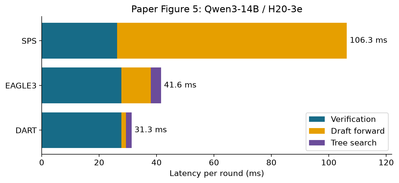
Figure 6. Redrawn from paper Figure 5. These are per-round stage measurements for Qwen3-14B. SPS has a different draft horizon, so the bars are useful timing diagnostics rather than a controlled single-variable architecture comparison.

The neural draft ratio is $10.2/1.5=6.8$. Including search, the draft-side ratio is $13.8/3.5\approx3.94$. Including target verification, the round-time ratio is $41.6/31.3\approx1.329$. These three ratios answer different questions. Comparing only the first pair would substantially overstate the effect on user-visible decoding time.

Using the table’s acceptance lengths as a rough common convention gives an illustrative combined estimate

$$\frac{S_D}{S_E}\approx \frac{3.67}{3.48}\frac{41.6}{31.3}\approx1.40. \tag{12}$$

The reported ratio of mean speedups is $2.77/2.02\approx1.37$. I do not interpret the small difference as an inconsistency: the timing figure and table use aggregated measurements, and a ratio of means need not equal a mean of ratios. The calculation serves to show the two multiplicative contributions: less time per round and modestly more accepted progress.

Verification accounts for $27.8/31.3\approx88.8\%$ of DART’s measured round time. Even deleting all remaining draft and search cost while holding accepted progress fixed would yield only $31.3/27.8\approx1.126$ further speedup in that example. This is an Amdahl-style bound under fixed workload and acceptance assumptions. Once drafting becomes cheap, target verification is the next dominant cost.

There is a useful inequality for deciding whether a more accurate but slower draft helps. Let a baseline round have progress $M$ and time $T$. A modification adds $\Delta M$ progress and $\Delta T$ time. Its throughput improves only if

$$\frac{M+\Delta M}{T+\Delta T}>\frac MT \quad\Longleftrightarrow\quad \frac{\Delta M}{M}>\frac{\Delta T}{T}, \tag{13}$$

assuming positive denominators. This is why larger trees, longer horizons, and stronger continuity models should be evaluated as a joint budget. Acceptance improvement is valuable only when it outweighs additional work. DART’s principal contribution is to improve this tradeoff, not to maximize one isolated accuracy metric.

8. What the main experiments establish

The main hardware description is a server with eight H20-3e GPUs of 141 GB each, 90 CPU cores, and 900 GB host RAM. That is the available training/inference server configuration; it should not be casually rewritten as proof that every reported target run uses all eight GPUs. Appendix F separately identifies a single A100-40G evaluation. Main results default to batch size one, with seven benchmarks spanning conversation, instruction following, mathematics, and code.

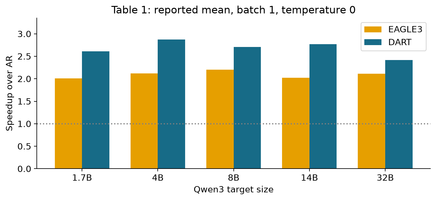
Figure 7. Redrawn from paper Table 1. Mean speedup across seven tasks at batch one and temperature zero. Values are relative to ordinary autoregressive decoding for each target. This figure does not compare absolute throughput across target sizes.

For the five Qwen3 targets, dividing each DART mean speedup by the matching EAGLE3 value yields improvements of approximately 29.9%, 35.4%, 23.2%, 37.1%, and 14.7%. Their simple arithmetic mean is about 28.1%. This is consistent with the paper’s broad “around 30%” description, but it is a specific recomputation from displayed means, not necessarily the authors’ aggregation method over all runs.

CodeAlpaca on Qwen3-14B gives $3.44/2.08-1\approx65.4\%$, explaining the highlighted 65% advantage. A different workload can give a smaller gain: Math500 on Qwen3-32B gives $2.46/2.31-1\approx6.5\%$. Domain and model size change the balance; the best example is not a general service-level promise.

The abstract’s 2.03–3.44× range should also not be treated as an exhaustive bound over every reported cell. Table 1 includes 3.45× on Qwen3-4B CodeAlpaca at temperature zero and 1.84× on Qwen3-32B Alpaca at temperature one. The table is the more precise source for a particular condition. Small discrepancies in headline ranges should be reported plainly rather than silently harmonized.

At temperature one, DART’s means are 2.47× for Qwen3-14B and 2.19× for Qwen3-32B, compared with EAGLE3’s 1.89× and 1.97×. This broadens the evidence beyond greedy decoding, though it does not substitute for a detailed statistical validation of the tree sampler. The paper omits generation-quality comparisons because it treats the procedure as distribution-preserving. That is reasonable under a correct verifier, but it makes the exactness assumptions important to state clearly.

The LLaMA2-Chat-7B experiment compares DART with PLD, Lookahead, Medusa, and Hydra, and reports 2.85× mean speedup for DART versus 2.66× for Hydra. The Qwen3 comparisons do not include all those methods because the paper reports compatibility constraints. Accordingly, I would not present the full table as a single uniform benchmark of every method on every target. Baseline availability is a practical constraint and a limitation on the strength of cross-family conclusions.

9. Ablations: useful evidence with incomplete uncertainty

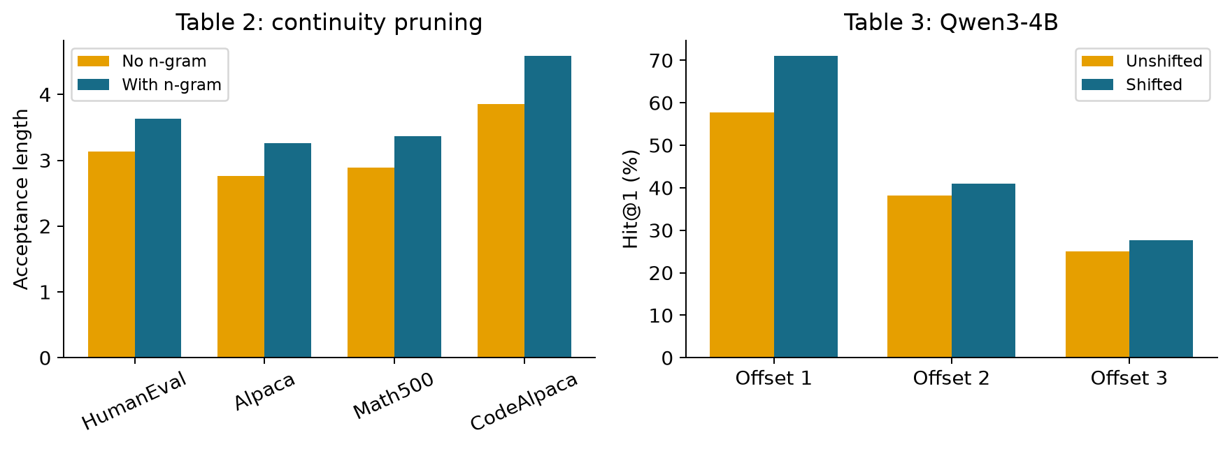
Figure 8. Redrawn from paper Tables 2–3. The left panel measures acceptance length with and without n-gram pruning. The right panel measures single-position hit@1 under shifted versus unshifted prediction. These are distinct metrics, and neither alone is a wall-clock speedup.

The n-gram ablation increases acceptance from 3.13 to 3.63 on HumanEval, 2.76 to 3.26 on Alpaca, 2.89 to 3.37 on Math500, and 3.85 to 4.59 on CodeAlpaca. Relative gains are approximately 16.0%, 18.1%, 16.6%, and 19.2%. This supports the usefulness of local continuity during tree selection. Table 2’s caption does not give every configuration detail, so it should not be treated as a fully specified isolated experiment without the surrounding method context.

Shifted prediction raises first-offset hit@1 from 57.7% to 71.1% on Qwen3-4B: a 13.4 percentage-point gain, not a 13.4% relative gain. Later offsets improve from 38.1% to 41.0% and from 25.1% to 27.6%. Top-10 coverage also improves, reaching 93.2%, 76.7%, and 65.9% for the first three offsets. These values support keeping multiple candidates, but they do not prove that every extra top-10 token belongs to an accepted joint path.

The position-weight sweep is more subtle. $\gamma=0.5$ has the highest first-position accuracy in Table 4, 76.2%, yet $\gamma=0.6$ has the highest acceptance length, 3.63 versus 3.59. Optimizing only the first prediction would therefore miss the best measured tradeoff. The difference is small, and no confidence interval or multi-seed variance is supplied. I would treat 0.6 as the reported default with empirical support, not a universally optimal constant.

The ablations do not isolate every mechanism. A factorial study crossing shifted prediction, KL decay, n-gram weight, tree size, and beam width would reveal interactions. For example, a broader tree could compensate for weaker individual logits, while a smaller tree might make early-position weighting more important. The paper demonstrates that its chosen components help in its comparisons; it does not establish that each component has an independent additive effect across all resource budgets.

10. Batching and hardware change the answer

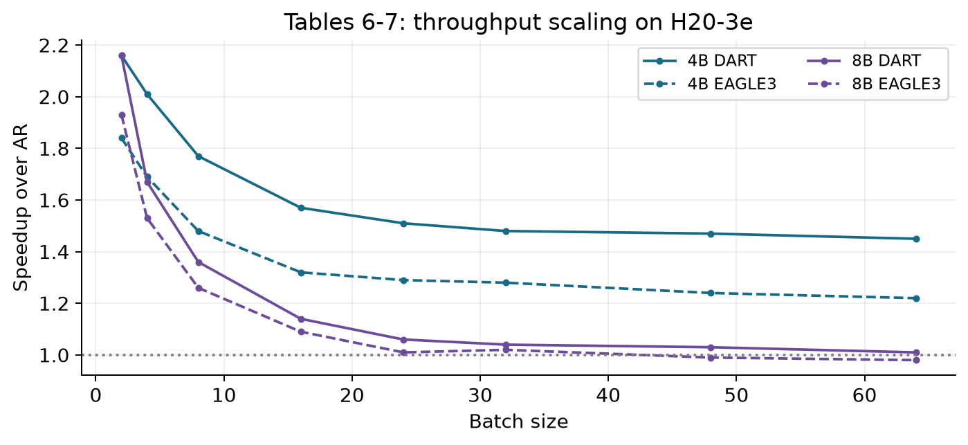
Figure 9. Redrawn from paper Tables 6–7. Speedups use each target’s ordinary decoding baseline. Qwen3-4B retains a substantial gain at batch 64, while Qwen3-8B approaches parity. Dashed lines denote EAGLE3, solid lines DART.

At batch 64, Qwen3-4B throughput is 370.0 tokens/s for the baseline, 453.3 for EAGLE3, and 538.7 for DART. Qwen3-8B gives 360.3, 356.4, and 366.1 tokens/s respectively. Direct division gives $366.1/360.3\approx1.016$, displayed as 1.01× in the paper, and $356.4/360.3\approx0.989$, displayed as 0.98×. The ratios may reflect precision or measurement aggregation not fully visible in the rounded table. The practical conclusion is robust: the 8B advantage is small at that batch size.

Batching raises arithmetic utilization of ordinary decoding and reduces the spare compute that speculation can exploit. A candidate tree adds verification positions, so its additional work becomes more costly when the GPU is already compute-bound. The presence of a faster draft does not make those extra target computations free. The table supports a workload-dependent switch between speculative and ordinary decoding, not a fixed rule that speculation is always preferable.

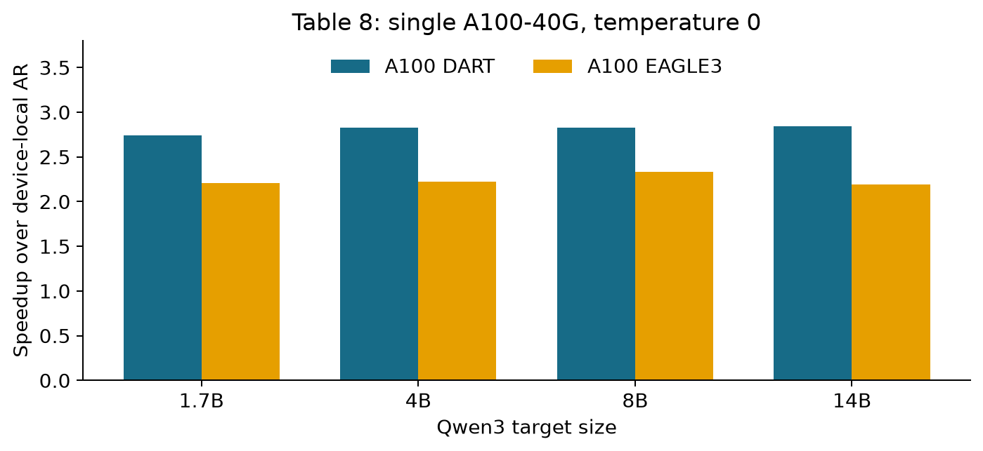
Figure 10. Redrawn from paper Table 8, single A100-40G, temperature zero. DART mean speedups range from 2.74× to 2.84× for the reported targets. These are device-local normalized speedups; they do not establish that an A100 has higher absolute throughput than an H20-3e.

Appendix F is useful because it shows that the benefit is not exclusive to one GPU generation. However, “hardware-agnostic” is a stronger phrase than the evidence warrants. Two GPU families with a particular host setup do not cover consumer memory capacities, heterogeneous NUMA layouts, different attention kernels, or large-model tensor-parallel deployments. The CPU index also means that portability has a host side as well as a GPU side.

For an adoption decision, I would ask for throughput, latency percentiles, and memory usage under the actual request distribution. A static batch-size experiment is informative but does not model arrivals, variable output lengths, queueing, prefill interference, or prefix reuse. A long generated answer amortizes startup work differently from a short answer. Those are ordinary serving variables, not reasons to dismiss the method; they define where its reported benefit needs to be retested.

11. Limitations and failure boundaries

The first boundary is target coupling. DART needs intermediate target features, a compatible tokenizer, and a trained drafter. It is not a drop-in accelerator for a black-box API that exposes only text or token probabilities. A target update can change the feature distribution and require re-evaluating draft alignment. The paper evaluates selected dense Qwen3 models and LLaMA2-Chat-7B; its results should not be assumed to transfer unchanged to MoE or hybrid recurrent architectures.

The second boundary is local statistical support. A trigram trained on a broad corpus can favor common code and language fragments, yet rare identifiers, specialized notation, unusual formatting, or domain-shifted text may lack useful support. Pruning then reduces acceptance rather than necessarily reducing output quality, provided target verification remains exact. This distinction matters: the primary failure mode should be wasted compute or lower speed, not a claim that the n-gram itself understands the task.

The third boundary is the resource envelope. Roughly 100 GB resident host memory is manageable on some inference servers and prohibitive on others. Cold loading, multiple tokenizer-specific indexes, memory pressure, and cross-socket traffic can change the total cost. The paper’s warm lookup measurements do not quantify all those scenarios. Training cost and index construction cost are also not included in decode speedup.

The fourth boundary is evidence granularity. Many results are point estimates without error bars. The exact definition of acceptance length, sampled tree verification, some score edge cases, and the scope of the main GPU allocation are not fully expanded in the presentation. Those are gaps in a reproducible method description, not evidence that the method fails. A careful review should neither erase them nor upgrade them into unobserved bugs.

Finally, the paper compares against methods available and compatible at its study time. It does not contain a controlled head-to-head comparison with every later parallel drafter. Relating DART to DFlash can clarify a design question, but a claim of superiority between them would require matched measurements. Similar terminology does not imply identical masks, teacher alignment, or tree construction.

12. Independent critical analysis

12.1 The strongest contribution is an allocation of dependency

I find the decomposition more important than the diffusion label. A target-coupled feature model produces marginals cheaply; a host-side local model restores some dependency; the target resolves the remaining uncertainty. Each component operates at a different cost and fidelity. This gives a useful design principle: do not pay a neural forward pass merely to encode dependencies that a cheaper mechanism can approximate well enough for proposal ranking.

The converse is equally important. Trigram consistency is not semantic consistency in the strong sense. The paper sometimes uses language suggesting globally coherent continuations, but a three-token statistic cannot generally enforce a variable binding or argument structure spanning a long context. A clearer claim would be that short-context continuity improves the candidate set before exact target evaluation. That narrower claim is both technically meaningful and well supported by the ablation.

12.2 Bidirectionality is not itself a violation of exact sampling

The paper motivates causal drafting by contrasting it with bidirectional diffusion models. As a design choice this is sensible: the known prefix is the only factual context, and iterative denoising can be expensive. But a proposal mechanism can use bidirectional communication among its own masked or proposed future positions without necessarily violating exact target sampling. The decisive requirements are that it does not use unavailable ground-truth future information and that its verification/correction mechanism is valid for the proposal process.

The distinction separates an engineering choice from a mathematical necessity. Causal masking helps align DART’s training and inference and keeps the design simple. It is not a general theorem that every noncausal drafter must bias the output. The same logic applies to the n-gram score: arbitrary ranking can be useful, but correctness must come from the verifier rather than from the plausibility of that ranking.

12.3 Optimize the marginal value of a candidate, not only its score

The fixed $(d,k,w,\theta)=(8,25,20,59)$ configuration is understandable for a controlled evaluation. In a serving system, the best candidate budget could vary with prefix uncertainty, batch occupancy, and measured host latency. A node that adds a tiny chance of extending an already likely path may be worth more or less than a new branch at an early depth. Ranking by a static cumulative score does not directly optimize expected committed tokens per verification millisecond.

A useful research objective would be to maximize an estimated progress gain minus its resource cost. For example, for a candidate expansion $u$, define the conceptual utility

$$U(u)=\widehat{\Delta\mathbb E[M]}(u) -\eta_V\widehat{\Delta T_V}(u) -\eta_S\widehat{\Delta T_S}(u). \tag{14}$$

This is my proposed objective, not part of DART. The multipliers encode the operating point, and the estimates would need calibration. A practical study should compare such adaptation with a fixed budget under identical target outputs, including the controller’s own overhead. A controller that spends more time deciding than it saves is not an improvement.

12.4 The next experiment should expose the whole resource frontier

I would first vary index size, coverage, and n-gram order at a fixed verification-node budget. Report RAM, cold-start time, warm lookup latency, per-round search time, acceptance length, and end-to-end speed together. This would show whether 100 GB is essential for the observed gain or one convenient point on a wider frontier. It would also distinguish better local statistics from simply spending more memory.

Next, cross domain with resource pressure: code, ordinary chat, mathematical text, and rare domain-specific identifiers, each under isolated and concurrent CPU load. That tests the paper-specific assumption that cheap continuity remains cheap and useful. Report tokenization and corpus provenance so that unusually strong code results can be interpreted without conflating useful corpus statistics with an unmeasured notion of semantic generalization.

Finally, a precise sampled-verification description would strengthen the paper at low additional conceptual cost. State the proposal process after pruning, acceptance rules, residual or fallback behavior, ancestor closure, and temperature handling. A small-vocabulary analytical example can demonstrate distribution conservation directly. Such an explanation would make the lossless claim inspectable from the method itself, independent of any particular implementation.

13. Conclusion and reading checklist

DART provides a concrete answer to a real bottleneck: make the neural drafter parallel, then use structured local statistics to recover useful candidate sequences. Its evidence supports meaningful single-request acceleration, with especially favorable code-generation examples, while showing that acceptance length alone is the wrong optimization target. The most valuable lesson is to count the full round: draft forward, tree construction, verification, and committed progress.

My adoption checklist would contain five questions. Is the target accessible at the required feature layers? Is the host memory and NUMA budget compatible with the index? Does the workload still have spare verification compute? Is sampled output preservation specified for the actual tree procedure? And does the measured gain survive the real arrival and length distribution? A positive answer to those questions would make DART a strong candidate; a good batch-one plot alone cannot answer them.

This review explains and independently analyzes the paper’s reported method and measurements. All additional formulas, arithmetic comparisons, and toy examples are identified as derivations or illustrations. No new model-training or inference benchmark result is claimed.

References and evidence map

• Liu et al., DART, arXiv:2601.19278v1, 2026-01-27. Read the complete 15-page PDF, including Appendices A–G. Sections 3–4 support the architecture, loss, and pruning discussion; Figure 5 and Tables 1–8 support the numerical comparisons; Appendices B–D support training and index details.
• Leviathan, Kalman, and Matias, Fast Inference from Transformers via Speculative Decoding. Background for acceptance-and-correction reasoning. Equations (3)–(4) provide the self-contained single-token calculation used here.
• DART official resource entry, linked by the paper. Included as a resource pointer.
• Figures 1–3 and 5 are original explanatory constructions. Figure 4 combines a calculated weight curve with Table 4 data. Figures 6–10 redraw explicitly identified paper measurements. Equations (1)–(4), (6), (8)–(9), and (11)–(14) are explanatory derivations or proposed analysis; they are not new empirical results.