TTT-Discover: Learning During Search for One Exceptional Solution

Review date: 2026-10-13
Paper: Learning to Discover at Test Time (TTT-Discover)
Authors: Mert Yuksekgonul, Daniel Koceja, Xinhao Li, Federico Bianchi, Jed McCaleb, Xiaolong Wang, Jan Kautz, Yejin Choi, James Zou, Carlos Guestrin, Yu Sun
Identifier and version: arXiv:2601.16175v2, 2026-02-05; first submitted 2026-01-22
Resources: Full paper and appendices · Author project · Official resource

1. The question: can the searcher improve while searching?

A language model can propose thousands of candidate solutions without changing the distribution that produced them. A search system can improve this process by retaining good candidates and feeding them back into the next prompt. TTT-Discover adds another form of memory: it updates the model’s weights using experience from the very problem it is trying to solve. The final deliverable is a candidate solution, such as a mathematical construction or an optimized program. The adapted policy is a tool used to find that candidate.

This change matters when a problem admits repeated, informative evaluation and one exceptional result is valuable. A kernel designer needs one correct fast kernel, not a model that produces moderately fast kernels reliably on unrelated tasks. A mathematical search may need one feasible construction that tightens a bound, even if most sampled constructions are poor. In that setting, average reward and the quality of the best discovered solution can favor different search behavior.

The paper combines two specific mechanisms. An entropic objective gives unusually good outcomes disproportionate influence on learning, while an adaptive temperature limits the concentration of that influence. A PUCT-inspired archive rule chooses promising starting solutions while discouraging repeated expansion of a single lineage. Their interaction is the main methodological claim: learning improves proposals, and reuse lets improvements accumulate across proposals.

The experiments are substantial but heterogeneous. The strongest results include tighter constructive bounds and faster TriMul kernels. Other tasks match prior results or fail to exceed them. The paper does not establish a general autonomous scientist, nor does it need that interpretation to be interesting. My central conclusion is narrower: for expensive, continuously scored search problems, tailoring both learning and state selection to the best-result objective can be much more effective than simply running conventional test-time RL from scratch.

All numerical comparisons below refer to the selected v2 paper. Results are reported by its authors; the original diagrams and explicit toy calculations explain the method. Where the main text, tables, and appendix differ, I preserve the distinction rather than silently combining incompatible numbers.

2. Prerequisites: three objects that should stay separate

The first object is the problem description $d$. It defines what a solution should do, which constraints it must satisfy, and how it is scored. The second is the state $s$: an actual candidate solution. In mathematics, this can be a numerical array representing a step function. In program search, it can be program text. The third is the action $a$: a model response containing reasoning and code. Parsing or executing that response produces the next state.

The distinction between action and state is useful. A Python program that searches for a step function is not itself the final mathematical construction. Executing it produces the array that is scored. For kernel engineering, parsing the generated program yields the candidate kernel; evaluation then checks its behavior and runtime. Different domains can therefore share the same outer algorithm while using very different transition and reward procedures.

Let $T$ denote the transition and let $r_\star$ be the best known reference reward. A compact restatement of the task is:

$$a\sim\pi_\theta(\cdot\mid d,s),\qquad s'=T(s,a),\qquad r=R(s'),\qquad \text{discovery if }R(s')>r_\star. \tag{1}$$

Higher reward is always preferred in this notation. A minimization metric such as runtime must be transformed accordingly; the paper often uses its reciprocal. An invalid or timed-out candidate receives zero. That convention assumes valid outcomes are assigned a compatible positive reward. The validity predicate is part of the problem, not a detail that can be removed from the optimization.

A policy-gradient update changes the probability of sampled responses. It does not differentiate through a GPU benchmark, a compiler, or a numerical solver. For a response consisting of tokens, its log probability is a sum of conditional token log probabilities. A response-level advantage can consequently influence many token decisions, even though the evaluator supplies one scalar after the response is complete. This is one reason long responses and noisy rewards can make credit assignment difficult.

State reuse supplies an effective multi-step horizon. A successful candidate becomes the starting point for a later attempt, whose child can in turn become another parent. Each generated response remains a bounded attempt, but the archive preserves work that would otherwise have to fit inside a single context window. Weight updates and archive updates play complementary roles: one changes the proposal distribution, and the other changes the concrete material presented to it.

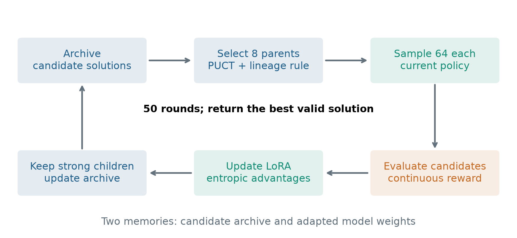
Figure 1. Original method diagram based on Sections 2–3 and Appendix A. The batch configuration is 8 parents with 64 rollouts each, repeated for 50 training rounds. The final output is the best valid solution observed.

3. Why maximizing the mean can miss the discovery objective

Consider an explanatory example, not an experiment from the paper. A safe policy always receives reward 3. A risky policy receives reward 10 with probability $1/8$ and zero otherwise. Their expected rewards are 3 and 1.25, respectively. If discovery requires a reward above 5, however, the safe policy cannot succeed. Under independent sampling from the risky policy, the probability of at least one discovery after $N$ attempts is:

$$\Pr\!\left(\max_{1\leq i\leq N}R_i>5\right) =1-\left(1-\frac18\right)^N. \tag{2}$$

This expression follows by computing the probability that every attempt fails and subtracting it from one. Independence is an assumption of this toy example; TTT-Discover’s attempts are dependent because both the policy and starting states change. The example nevertheless demonstrates a real mismatch between optimizing average reward and optimizing the chance of an exceptional outcome.

The paper also points out a scale problem. Improving a kernel from 2000 to 1900 microseconds can be a meaningful engineering advance, yet the difference between their raw reciprocal rewards is small. A fixed-temperature exponential objective can become insensitive to these small late-stage differences. Conversely, a large fixed temperature early in training can let one outlier dominate the update.

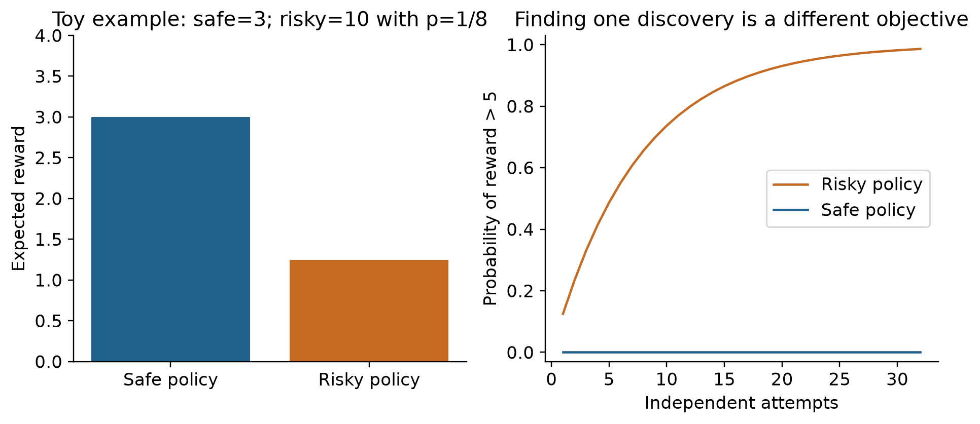
Figure 2. Analytical illustration with invented reward distributions, explicitly separate from the paper’s experiments. The discovery threshold is 5; the risky policy produces reward 10 with probability 1/8.

There is a limit to the argument. A preference for the upper tail does not automatically maximize the expected best result at a fixed total cost. It can overvalue extremely rare events, reward noise, or expensive proposals. TTT-Discover uses an entropic surrogate and an archive heuristic; it does not solve the finite-budget best-result objective exactly. That distinction becomes important when interpreting its theoretical motivation.

4. Deriving the entropic policy gradient

For a fixed starting state, define a partition function and its logarithm:

$$Z_\beta(\theta;s)=\sum_a\pi_\theta(a\mid s)e^{\beta R(s,a)}, \qquad J_\beta(\theta;s)=\log Z_\beta(\theta;s). \tag{3}$$

The problem description is suppressed in the notation. During this derivative, the current state, reward function, and selected inverse temperature $\beta$ are treated as fixed. This is the local update used by the method; it does not differentiate through the full history of archive selection or the procedure that selected $\beta$.

Apply the chain rule, then use $\nabla\pi=\pi\nabla\log\pi$:

$$\begin{aligned} \nabla_\theta J_\beta &=\frac{1}{Z_\beta}\sum_a e^{\beta R(s,a)}\nabla_\theta\pi_\theta(a\mid s)\\ &=\sum_a\pi_\theta(a\mid s) \frac{e^{\beta R(s,a)}}{Z_\beta}\nabla_\theta\log\pi_\theta(a\mid s)\\ &=\mathbb E_{a\sim\pi_\theta}\!\left[w_\beta(a)\nabla_\theta\log\pi_\theta(a\mid s)\right]. \end{aligned} \tag{4}$$

The weight is an exponential reward divided by its expectation. Its population mean is one. Also, the expectation of the score function $\nabla\log\pi$ is zero. Subtracting one from the weight therefore leaves the population gradient unchanged and yields a centered advantage:

$$w_\beta(a)=\frac{e^{\beta R(s,a)}}{Z_\beta},\qquad A_\beta(a)=w_\beta(a)-1. \tag{5}$$

A response above the exponentially weighted reference level receives positive pressure; other responses can receive negative pressure. This differs from simply subtracting the arithmetic mean reward. Relative differences in the upper tail matter exponentially, and the strength of that preference depends on $\beta$.

Two limiting calculations clarify the design. Around zero, the cumulant expansion gives:

$$\frac{J_\beta}{\beta} =\mathbb E[R]+\frac{\beta}{2}\operatorname{Var}(R)+O(\beta^2). \tag{6}$$

For small positive $\beta$, the normalized objective favors both a high mean and dispersion toward high outcomes. This is a mathematical explanation, not a claim that arbitrary variance is beneficial. For large $\beta$, with a finite support and positive policy mass on the maximizing action, factoring out the largest exponential gives:

$$J_\beta =\beta R_{\max}+\log\!\sum_a\pi_\theta(a\mid s) e^{\beta(R(s,a)-R_{\max})},\qquad \lim_{\beta\to\infty}\frac{J_\beta}{\beta}=R_{\max}. \tag{7}$$

The normalization matters. The unnormalized logarithm generally grows with $\beta$; it does not literally converge to the maximum reward. The paper’s informal statement that the objective tends to the maximum should be understood through this normalized limit, or the corresponding concentration of its weights. Nor can exponential reweighting create an action to which the current policy assigns no probability.

5. Adaptive temperature: constrain the tilted distribution

The method defines an auxiliary distribution by tilting the current policy toward high rewards:

$$\begin{aligned} q_\beta(a\mid s)&=\pi_\theta(a\mid s)w_\beta(a),\\ D_{\mathrm{KL}}(q_\beta\Vert\pi_\theta)&=\gamma,\qquad\gamma=\log 2. \end{aligned} \tag{8}$$

This is one KL quantity. The method also uses a penalty relative to the initial model in its learning advantage. That is a second KL-related mechanism with a different purpose. The first controls how concentrated the outcome weights become within a state; the second discourages policy drift away from the initial model. A constraint on $q_\beta$ does not by itself guarantee an exact trust-region bound on the neural policy after an optimizer step.

For a group of $K=64$ sampled responses, the empirical reference distribution is uniform over those samples. The normalized weights and constraint become:

$$q_n(\beta)=\frac{e^{\beta r_n}}{\sum_{m=1}^{K}e^{\beta r_m}},\qquad D_{\mathrm{KL}}(q\Vert u)=\sum_{n=1}^{K}q_n\log(Kq_n) =\log K-H(q). \tag{9}$$

The last equality provides an intuitive interpretation. When the constraint is met, $H(q)=\log(K/2)$, so the entropy-effective support $e^{H(q)}$ equals 32 for a group of 64. This is not a guarantee that exactly 32 samples receive nonzero weight. It is also not the usual importance-sampling effective sample size $1/\sum q_n^2$. These quantities describe different aspects of concentration.

Why does bisection work? With $Z$ defined over the finite batch, the divergence is $\beta\mathbb E_q[r]-\log Z+\log K$. Differentiating yields:

$$\frac{d}{d\beta}D_{\mathrm{KL}}(q_\beta\Vert u) =\beta\operatorname{Var}_{q_\beta}(r)\geq0. \tag{10}$$

Thus concentration increases monotonically with nonnegative $\beta$, except on flat regions. The equality constraint need not be attainable. If all rewards tie, $q$ remains uniform for every temperature. If $k$ outcomes share the maximum reward, the limiting divergence is $\log(K/k)$, which can be smaller than the requested budget. A complete numerical procedure must handle these cases explicitly; the paper states the bisection rule without specifying every degenerate-case convention.

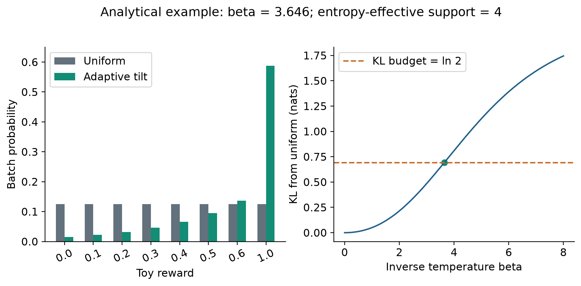
Figure 3. Original numerical illustration using eight stated toy rewards. The KL target is log 2, making the entropy-effective support four. This calculation illustrates Appendix A.1; it is not a training result.

Appendix A.1 uses a leave-one-out denominator for the advantage. Subtracting the maximum reward stabilizes exponentiation without changing normalized ratios:

$$z_n=e^{\widehat\beta(r_n-r_{\max})},\qquad \widehat Z_{-n}=\frac{1}{K-1}\sum_{m\ne n}z_m,\qquad \widehat A_n=\frac{z_n}{\widehat Z_{-n}+\epsilon}-1. \tag{11}$$

Leaving the current sample out avoids using its own unusually large reward to inflate its denominator. It does not make the estimator identical to the population advantage. In a finite batch the advantages need not sum to zero, and a ratio estimator is not generally unbiased. In particular, the concentration constraint is imposed on the full-batch $q$, while the learning advantages use leave-one-out normalization. Those should not be described as the same normalized weights.

For a positive affine transformation $r'_n=a r_n+b$, choosing $\beta'=\beta/a$ leaves $q$ unchanged. The reward shift cancels in normalization and in the stabilized leave-one-out exponentials. This explains the claimed scale and shift invariance, subject to numerical tolerances and temperature-search limits. It does not imply invariance to nonlinear transformations such as replacing reciprocal runtime with negative runtime.

Algorithm 1. Adaptive entropic advantages for one parent

1. Input rewards r[1:K] from one shared starting state.
2. Define q(beta) = softmax(beta * r).
3. Find beta >= 0 with KL(q || uniform) = log(2).
4. Use bisection when the target is attainable.
5. If rewards tie or the target is unreachable, handle
   that case explicitly; no infinite-temperature search.
6. Set z[n] = exp(beta * (r[n] - max(r))).
7. For each n, compute Z_loo = mean(z[m] for m != n).
8. Set A[n] = z[n] / (Z_loo + epsilon) - 1.
9. Add the reference-policy penalty during learning.

Steps 1–4 and 6–9 restate the paper’s estimator; step 5 identifies a mathematical boundary that any finite numerical treatment needs. It is not a claimed additional rule from the authors. A group in which all candidates are invalid contains no relative improvement signal. Increasing the inverse temperature cannot manufacture that missing information.

6. State reuse: optimistic values with lineage-aware exploration

The archive is more than a list of best scores. It records parent-child relationships, visits, and evidence about which states produce good descendants. Appendix A.2 gives the complete selection score, including a reward-range scale factor omitted from the abbreviated main-text expression:

$$S(s)=Q(s)+c\,\Delta R\,P(s)\frac{\sqrt{1+T}}{1+n(s)}, \qquad \Delta R=R_{\max}-R_{\min}. \tag{12}$$

Here $T$ counts expanded parents, $n(s)$ counts expansion visits accumulated through the lineage, and $c=1$ in the reported setup. The first term exploits a state’s demonstrated potential. The second gives a larger bonus to relatively promising, insufficiently explored states. Multiplying by the reward range helps keep the bonus in the same units as the exploitation term.

For an archive of size $M$, rewards determine a descending rank beginning at zero. The prior is:

$$P(s)=\frac{M-\operatorname{rank}(s)}{\sum_{j=1}^{M}j} =\frac{2\bigl(M-\operatorname{rank}(s)\bigr)}{M(M+1)}. \tag{13}$$

The best state receives $M$ times the prior of the lowest-ranked state. Every archived state still receives positive prior mass. A rank prior is less sensitive to an isolated reward outlier than a reward softmax, but it discards information about the magnitude of gaps. The reward-range factor only partially restores a notion of scale; it does not make the prior sensitive to local score spacing.

For an unvisited state, $Q(s)$ is its own reward. For a visited parent, it is the maximum observed reward among its directly generated children. The use of a maximum fits the best-result goal, but makes the value susceptible to measurement noise. The appendix updates that best-child statistic only for the direct parent. It propagates visit counts to all ancestors. Propagating a maximum reward through every ancestor would be a different rule.

Within a batch, selecting a parent blocks its ancestors and descendants from being selected as other parents. This prevents a batch of eight groups from spending most of its capacity on near-identical stages of one search route. After expansion, the archive retains the best two children per parent and applies a top-1000 reward-based limit while preserving initial seeds. The resulting algorithm favors successful lineages without allowing them to occupy every current starting point.

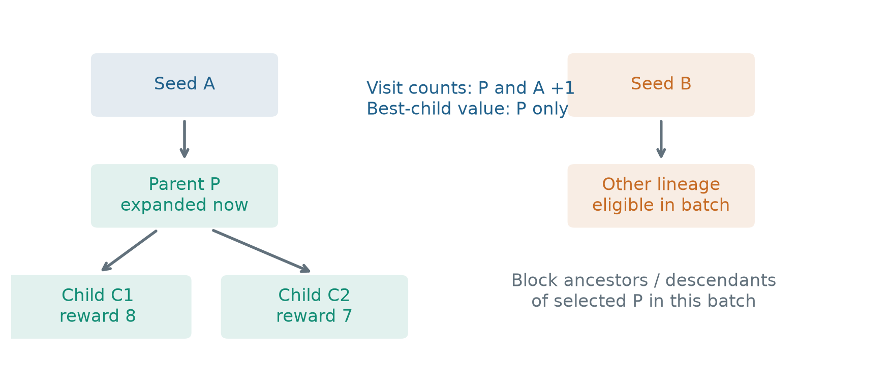
Figure 4. Original schematic of Appendix A.2. The child rewards 8 and 7 are illustrative. Lineage blocking applies to parent selection within the current batch, while visit accounting persists across batches.

Algorithm 2. Archive selection and update

1. Rank current archive states by reward; compute P(s).
2. Form S(s) from Q, reward range, prior, and visits.
3. Select a high-scoring eligible parent for a group.
4. Block its ancestors and descendants for this batch.
5. Repeat selection until the parent batch is formed.
6. Generate and evaluate each parent's child group.
7. Update each direct parent's maximum child reward.
8. Increment visits of that parent and its ancestors.
9. Increase the global expanded-parent count.
10. Insert the top two children from each parent.
11. Retain the top 1000 states, preserving seed states.

This is PUCT-inspired archive prioritization, not ordinary AlphaZero tree search. Its prior comes from candidate rank rather than a learned action policy, its value is optimistic rather than an average return, and the archive can prune states. Standard tree-search convergence claims do not automatically apply. If the reward range collapses to zero, the exploration bonus in Equation 12 disappears; tie handling and seed diversity then become important.

An alternative is epsilon-greedy reuse: mostly expand the current best state and occasionally sample elsewhere. It is simpler, and the paper’s kernel ablation shows it can work well. Its weakness is that a single early winner can monopolize exploitation without a nuanced account of which branches remain underexplored. Conversely, the top-two and top-1000 filters can discard a temporarily weak stepping stone that would have led to a better region later. TTT-Discover chooses a practical optimism-diversity tradeoff, not exhaustive exploration.

7. Putting learning and search together

The main experiments use gpt-oss-120b with LoRA rank 32 on Tinker. Each of 50 rounds produces 512 rollouts, grouped as eight starting states with 64 responses per state. The adaptive temperature is computed within each group. The paper takes one gradient step on the full batch and applies importance-ratio correction for a sampler/learner mismatch in the training infrastructure. This correction does not mean that the method repeatedly trains on arbitrary old archive responses.

The reference-policy term is written in the main text as:

$$A(a;s)=w_\beta(a)-1 -\lambda\log\frac{\pi_\theta(a\mid s)}{\pi_{\theta_0}(a\mid s)}. \tag{14}$$

The reference is the initial policy, while the entropic reweighting is defined relative to the current policy. The reported default coefficient is 0.1, reduced to 0.01 for algorithm engineering. The penalty helps retain a useful proposal distribution while the high-reward samples shape adaptation. It cannot guarantee that all language or reasoning capabilities survive arbitrary specialization.

Algorithm 3. The complete discovery loop

1. Input one problem, its evaluator, and initial policy.
2. Create domain-appropriate seed states and an archive.
3. For each of 50 training rounds:
4.   Select 8 eligible parents using Algorithm 2.
5.   Sample 64 responses from the current policy per parent.
6.   Parse or execute each response to obtain a candidate.
7.   Check validity; measure its continuous reward.
8.   Compute grouped advantages using Algorithm 1.
9.   Take one full-batch LoRA update with KL shaping
     and the stated sampler/learner ratio correction.
10.  Update parent statistics and retain strong children.
11. Return the best valid candidate observed in the run.

The order in this method-level pseudocode emphasizes the data dependencies. Evaluation must precede advantages, and the next sampling round uses the newly adapted policy and archive. Domain-specific prompts and execution budgets remain part of the environment; they are not learned by this outer procedure.

The default optimizer is Adam with learning rate $4\times10^{-5}$, moments 0.9 and 0.95, and epsilon $10^{-8}$. The context limit is 32,768 tokens. In most domains the prompt plus reasoning is limited to 26,000 tokens, reserving room for the final program. Appendix D changes that limit to 22,000 for AHC039 and 25,000 for AHC058, and reports a learning rate of $2\times10^{-5}$ for AHC058. The biology runs use a 20,000-token generation limit. These exceptions matter more than a blanket statement that every hyperparameter is identical across tasks.

There are also multiple execution-time descriptions. The main mathematics section describes a 10-minute limit; the appendix allows up to 1100 seconds, and example prompts mention 1000 seconds. These are documented differences, not a reason to choose one silently. They affect how much work one sampled response can perform after generation, so they belong in any careful reading of the compute comparison.

8. Mathematics: constructive improvements, with two important non-wins

In the Erdős minimum-overlap problem, one partitions a set into two equal parts and controls the largest number of differences at any offset. The paper follows a continuous formulation in which a bounded step function describes a limiting density. A feasible function supplies an upper bound on the limiting overlap constant. Its reported construction has 600 pieces and is asymmetric, unlike the earlier 95-piece construction discussed in the paper.

Table 2 reports 0.380927 for the previous best human upper bound, 0.380924 for AlphaEvolve, 0.380906 for Best-of-25600, and 0.380876 for TTT-Discover. Lower is better. The new value improves over both the prior reference and a strong same-model sampling baseline. However, Best-of-25600 already exceeds the earlier reference, so crossing that reference alone is not sufficient evidence for the unique value of online learning.

For the first autocorrelation inequality, the paper considers nonnegative functions with prescribed support. Any valid candidate supplies an upper bound through the ratio:

$$C_1\leq\frac{\lVert f*f\rVert_\infty}{\lVert f\rVert_1^2}. \tag{15}$$

The numerator penalizes the largest value of the autoconvolution, while the denominator removes an overall amplitude scale. A better candidate reduces the ratio subject to feasibility. The discovered search moves from gradient methods toward linear programming and focuses effort on nearly active convolution constraints. This explains why a tiny final improvement can reflect a meaningful change in optimization structure.

Table 2 gives 1.50287 for TTT-Discover, compared with 1.50317 for AlphaEvolve V2 and 1.50314 for the listed ThetaEvolve refinement. The prose and Figure 3 instead give 1.50286 for TTT-Discover. This review uses the table value for its comparison plot and records the last-digit discrepancy. The qualitative ordering is unchanged, but claiming a unique extra decimal would exceed the consistency of the source.

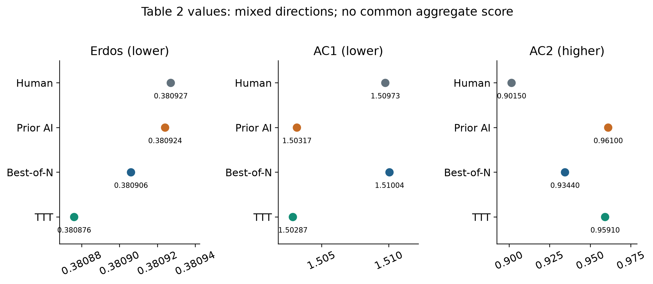
Figure 5. Original redraw of selected Table 2 values. The prior-AI reference is AlphaEvolve for Erdős and AlphaEvolve V2 for the two autocorrelation tasks. AC1 uses 1.50287 as printed in Table 2; the prose gives 1.50286.

The second inequality reverses the direction: a valid construction certifies a lower bound on a ratio involving the squared $L_2$ norm of the autoconvolution. TTT-Discover obtains 0.9591, below AlphaEvolve V2’s 0.9610, so it does not improve the best reference. Circle packing provides a second non-win. With Qwen3-8B, the method matches the best listed sums of radii, 2.635983 for 26 circles and 2.939572 for 32 circles, without exceeding them.

The small-model comparison with ThetaEvolve is informative but not perfectly matched. TTT-Discover uses the original Qwen3-8B, while ThetaEvolve uses a DeepSeek-distilled variant. The paper describes 50 training rounds of 512 rollouts versus 65 rounds of 512 for ThetaEvolve. It is therefore more precise to describe an encouraging comparison involving different model variants and budgets than to repeat the introduction’s loose same-model, same-compute characterization.

9. Kernel engineering: speedups depend on the measurement protocol

TriMul combines normalization, projections, gates, a large pairwise matrix operation, and another output transformation. The authors describe the discovered solution as reducing memory traffic through fusion, storing intermediate activations in FP16 where allowed, and delegating heavy matrix multiplication to optimized libraries. This is a sensible division of labor: the expensive arithmetic does not imply that replacing a mature matrix multiplication library is the best route to an end-to-end gain.

The search reward is measured on H100. Table 4 reports final performance on four GPU types. The A100 and H100 values come from official leaderboard submissions. B200 and MI300X values come from ten trials in an environment coordinated with the organizers, because the authors could not submit those runs through the official infrastructure. The distinction is part of the evidence, even though both sets of measurements are useful.

GPU	Best human runtime	TTT runtime	Derived speedup
A100	4531.5 microseconds	2198.2 microseconds	2.061×
H100	1371.1 microseconds	1161.2 microseconds	1.181×
B200	1038.9 microseconds	914.2 microseconds	1.136×
MI300X	2515.8 microseconds	1555.7 microseconds	1.617×

Speedup is the old runtime divided by the new runtime. Latency reduction is one minus the inverse of that ratio. For example, the A100 result corresponds to about 51.5% lower latency, while H100 is about 15.3% lower. The B200 table values imply about 12.0% lower latency, so they do not support an unqualified statement of greater than 15% improvement on every GPU. Earlier project-page numbers also differ; the table above consistently uses v2 Table 4.

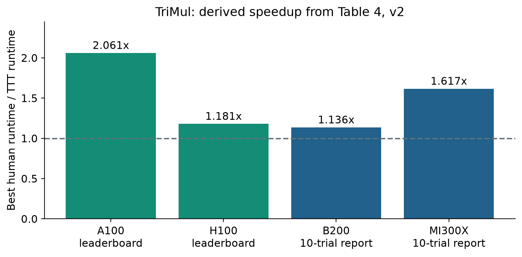
Figure 6. Ratios computed from v2 Table 4. B200 and MI300X use the reported mean runtimes from ten trials; the bars show ratios of means, not uncertainty intervals for speedup.

Hardware transfer requires an additional qualification. Appendix C selects candidates for target-hardware evaluation: H100 uses the top 20 training candidates; the other tasks combine high-scoring and randomly selected correct candidates at intervals. Candidates are then measured on the target hardware before a final choice. The learning reward comes from H100, but the final target-hardware candidate is not necessarily chosen without any target-hardware feedback.

MLA-Decode is a counterexample to a universal win. Training uses H200 because MI300X was unavailable at scale, while final evaluation uses three MI300X instances. Table 5 gives TTT runtimes of 1669.1, 1706.1, and 1671.3 microseconds; the best human means are 1653.8, 1688.6, and 1668.7. The authors explicitly report no statistically significant improvement over the best human result. A Triton-filtered subset is slower still in Appendix C.3.

Finally, passing the benchmark’s numerical tolerances is not equivalent to preserving every downstream workload’s numerical behavior. The expert commentary in the paper specifically raises FP16 stability as a potential limitation in full workloads. The result establishes a fast valid solution under the competition specification. It does not establish a universal drop-in replacement for every protein-model training or inference regime.

10. Algorithms and biology: held-out tests improve the evidence

For AHC039, the search starts from a strong existing ALE-Agent-derived program, matching the initial-state strategy used by ShinkaEvolve. For AHC058, it starts from scratch. These different starting points are essential context: the two tasks do not demonstrate the same degree of independent construction from an empty program.

Training uses 150 locally generated cases. The authors select their top three programs for final submission to the official platform, whose tests supply a distinct evaluation. Table 6 reports 567,062 for AHC039 versus the best human score of 566,997. The improvement is 65 points, about 0.0115%. For AHC058, 848,414,228 exceeds the listed ALE-Agent score of 848,373,282 by 40,946, about 0.00483%. These are narrow leaderboard improvements, not large practical margins.

The comparisons are retrospective. They show how the generated programs score against historical submissions; they do not mean the method entered and won those contests under their original wall-clock conditions. The reported discovered strategies combine familiar ingredients such as geometric candidate pools, greedy initialization, beam search, and simulated annealing. Novel value can arise from finding an effective combination, without every component being a new algorithmic invention.

The single-cell denoising task provides a different kind of held-out evaluation. The policy is optimized using Pancreas, while final algorithms are evaluated on PBMC and Tabula. Training begins with MAGIC. Appendix E constrains the normalized Poisson score to the interval from 0.97 to 1, then optimizes the MSE-related score. Table 1’s shorthand of reciprocal MSE should therefore not replace the more specific reward description in the appendix.

The composite benchmark score averages normalized MSE and Poisson components. It is different from the raw MSE and raw Poisson loss columns. For PBMC, TTT-Discover improves MSE from MAGIC’s rounded 0.19 to 0.15 and the composite score from 0.64 to 0.71. For Tabula, MSE changes from 0.18 to 0.14 and the composite score from 0.64 to 0.73. OpenEvolve is already close, with MSE 0.16 and 0.15 on the two datasets.

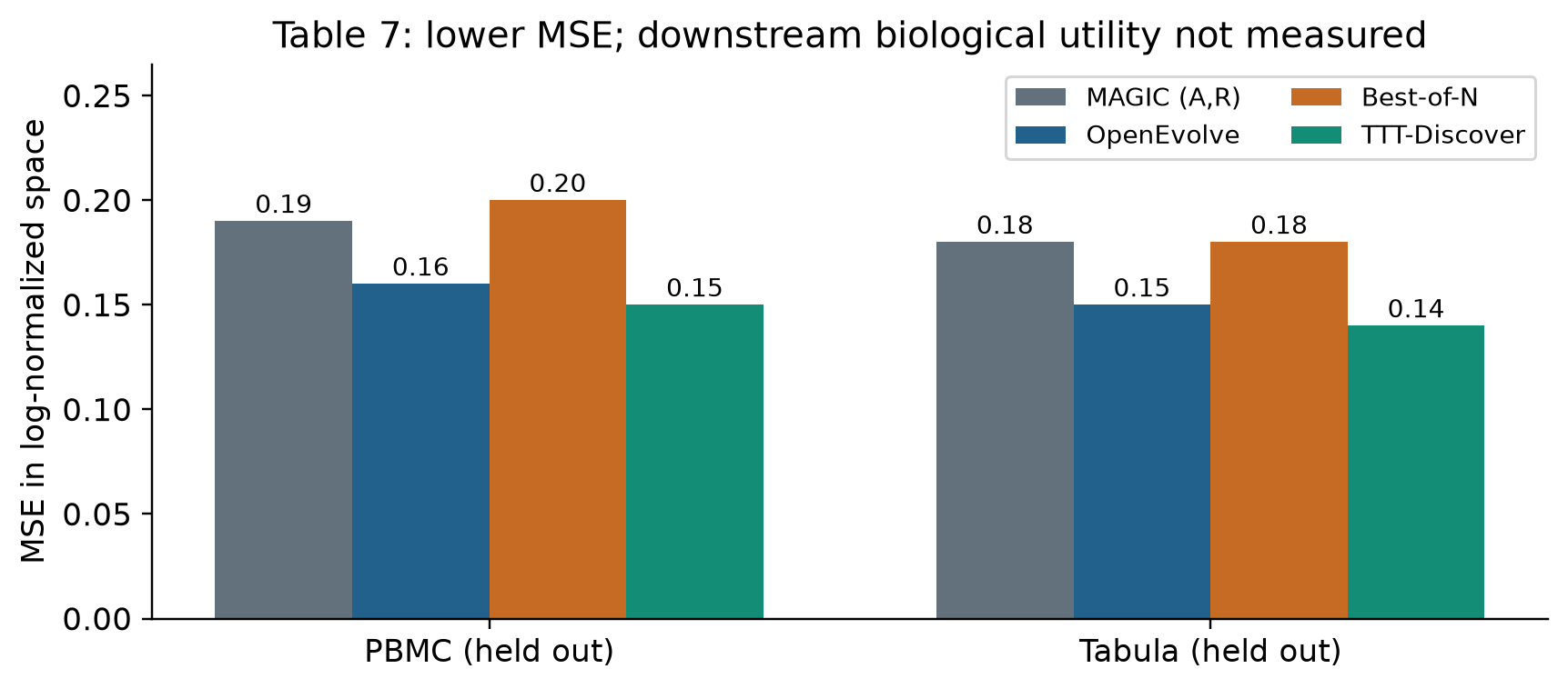
Figure 7. Original redraw of Table 7’s rounded MSE values. Pancreas supplies the training reward; PBMC and Tabula are held out. These benchmark improvements do not measure downstream biological discovery.

The authors describe gene-adaptive transform combinations, low-rank refinement, and log-space polishing. Those mechanisms plausibly improve the chosen reconstruction metric. They can also oversmooth weak but meaningful biological variation. The paper and its expert review explicitly separate improved benchmark metrics from validated biological insights. Held-out datasets strengthen the evidence for metric transfer, but do not close that downstream scientific gap.

There is a baseline caveat: the OpenEvolve run begins accumulating timed-out programs after roughly sample 17,000, and its best earlier candidate is retained. More generally, OpenEvolve’s growing prompts encounter the fixed context limit. This is a real system limitation under the selected protocol, but it makes the comparison less clean as a test of learning versus an equally well-adapted frozen-model search system.

11. What the ablations support

Table 8 is the clearest evidence about the proposed ingredients because it holds the model and rollout count fixed within one kernel task. The full method reaches a best local-evaluator runtime of 1203.10 microseconds. Fixed-temperature entropic learning with PUCT reaches 1483.83; expected-reward learning with PUCT reaches 1985.67; PUCT without learning reaches 2060.70. Adaptive learning with epsilon-greedy reuse reaches 1328.89, whereas removing reuse raises the runtime to 5274.03.

The naive RL and Best-of-N results, 5328.73 and 5352.36 microseconds, are close. In this configuration, merely allowing gradient updates is insufficient. The archive makes a particularly large difference, and adaptive entropic learning improves the strong reuse baseline. This pattern supports a joint system design, rather than the claim that weight updates alone explain the entire improvement.

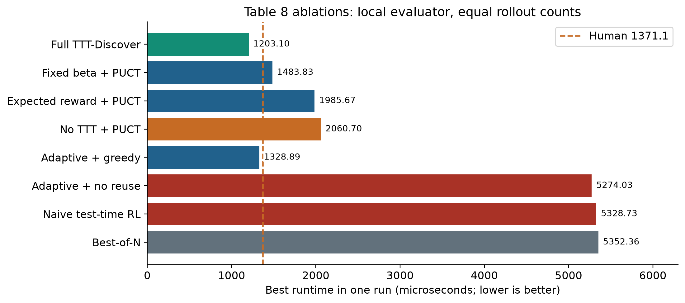
Figure 8. Original redraw of Table 8. These are best outcomes from individual runs under the local evaluator, not confidence intervals over independent training repetitions. The local full-method runtime differs from the 1161.2-microsecond official H100 result in Table 4.

The paper’s accompanying plots track the best-so-far reward, per-step mean reward, and per-step maximum. These answer different questions. A best-so-far curve cannot decrease by construction, even if the current policy deteriorates. A rising per-step mean suggests a more broadly improved proposal distribution, while the current maximum remains sensitive to luck. Reporting all three is useful, but none replaces repeated complete training runs when estimating reliability.

There are two especially important caveats. First, epsilon-greedy reuse performs reasonably well in this task, so the evidence for the exact PUCT variant is more modest than the evidence for reuse itself. Second, the ablations are not an exhaustive hyperparameter search: the authors acknowledge that alternative temperature schedules, batch sizes, and interaction effects could improve the weaker variants. A best result among these settings is not proof that the alternatives cannot compete.

The Figure 4 caption contains a simple arithmetic error: it prints 256,000 for 50 times 512. The correct product is 25,600, consistent with the main text and Best-of-25600 naming. This review uses 25,600 throughout. The correction changes the stated sampling budget by a factor of ten, so it is worth making explicit rather than copying the caption.

12. Compute accounting and a practical decision framework

Fifty rounds times eight parents times 64 responses gives 25,600 sampled attempts. Equal attempt counts control one part of the experiment. They do not imply equal generated-token counts, equal executed-program time, equal hardware cost, or equal human effort in constructing the problem evaluator.

The paper estimates about USD 500 on Tinker for a run with an average 3000-token prompt and 16,000 sampled tokens per response. That is a historical API estimate under the paper’s assumptions. It is not a current price quote, and it should not be read as a complete budget for all candidate execution, repeated target-device measurements, and expert evaluation.

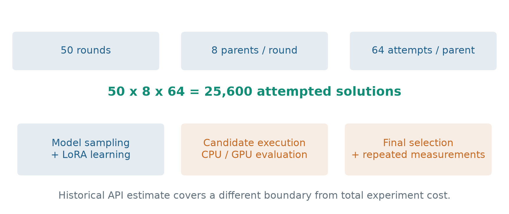
Figure 9. Original accounting diagram. The attempt count is exact for the standard configuration. The three expense categories explain why the paper’s API estimate and total experimental cost have different boundaries.

A useful accounting identity is:

$$C_{\mathrm{total}}= C_{\mathrm{sampling}}+C_{\mathrm{learning}}+ C_{\mathrm{evaluation}}+C_{\mathrm{selection}}+C_{\mathrm{setup}}. \tag{16}$$

This identity is my organizational model, not a new measured cost table. Candidate evaluation can dominate if each response launches a long optimization routine. As an upper-bound illustration only, 25,600 evaluations each consuming 1100 seconds would amount to about 7822 serial evaluator-hours. Actual programs may finish earlier, some candidates fail quickly, and parallel execution changes wall time. The calculation is useful precisely because it separates a worst-case resource envelope from an observed cost.

The method is most attractive when three conditions hold together. First, the evaluator provides a reliable graded signal. Second, the search horizon is long enough to amortize adaptation. Third, improvements can be carried forward as reusable candidate states. If feedback is binary and almost always zero, the exponential objective has little ranking information. If only a few attempts are affordable, a full adaptation loop may spend too much of the budget learning how to search.

The alternative choices are then concrete. Best-of-N offers simplicity and parallelism. Frozen-model evolutionary search offers reuse without gradient infrastructure. Test-time adaptation adds a changing proposal distribution but needs training access and optimizer stability. A learned value model could guide reuse more richly than rank, but would introduce its own prediction errors. The paper selects a relatively simple archive heuristic so that it can apply across very different evaluators.

For interpreting a future result, I would ask for a cost-normalized best-so-far curve, the fraction of valid completed candidates, a fixed final evaluation protocol, and repeated whole-run outcomes. These are experimental design questions about the method’s behavior. They distinguish an improved search process from a single fortunate sample and make different systems comparable even when their program-execution costs differ.

13. Limitations and failure boundaries

Continuous feedback is a substantive requirement. The authors identify sparse or binary rewards and non-verifiable domains as future work. When all 64 candidates receive zero, the adaptive temperature cannot discover which failed approach was closer to success. A curriculum, shaped reward, or a better state representation might help, but those would be additional mechanisms.

The evaluator can become the bottleneck in scientific validity. An optimizer that strongly favors maxima also strongly favors occasional measurement errors. Timing noise, permissive correctness tolerances, and proxy metrics can all create attractive false improvements. Repeated final evaluation mitigates some noise; it does not turn an incomplete biological metric into a complete description of biological usefulness.

There is no broad-generalization objective. The method specializes to one discovery problem. An improved candidate can transfer to new test cases, datasets, or hardware, as some experiments show, without the adapted language model becoming a generally better scientist. Candidate transfer and policy transfer are different claims and should be measured separately.

Archive pruning can remove useful stepping stones. The top-two child rule and global reward ranking prioritize immediate measured promise. Some routes require temporarily weaker candidates before a structural improvement becomes possible. Lineage blocking encourages diversity among retained states, but it cannot recover a path already pruned from the archive.

The reported hyperparameter robustness is bounded by the tested settings. Most values are shared across tasks, but there are documented changes in learning rate, KL coefficient, context allocation, and execution budgets. Model access also matters: systems restricted to a frozen inference API cannot directly use the weight-adaptation component.

The comparative evidence has uneven statistical depth. Some hardware measurements have ten-trial intervals, while the central ablation table reports a best solution per run. Confidence intervals for repeated timing of one selected kernel do not estimate the probability that a fresh complete search run will discover a comparable kernel. Selection variability and measurement variability require different repetitions.

14. Critical analysis: what is learned, and what is merely selected?

14.1 The contribution is a coupled optimizer

The convincing part of TTT-Discover is the alignment between objective and workflow. It does not merely attach standard RL to a generator. It tilts the learning signal toward unusually good outcomes and chooses starting states that can carry those outcomes forward. Table 8 suggests that these two choices reinforce each other. The archive supplies promising contexts; adaptation makes productive modifications more likely in those contexts.

Attribution remains incomplete. Reuse without learning already makes a large improvement over independent sampling. Adaptive learning without reuse barely improves this kernel result. The evidence supports an interaction, not a simple ranking in which learning universally replaces search. A useful next experiment would hold evaluator cost and valid completed samples fixed while comparing several strong reuse policies with and without adaptation. That would test whether the joint advantage survives better-tuned frozen-policy baselines.

14.2 The KL argument is informative but narrower than a trust-region guarantee

The adaptive rule has an elegant invariance and a clear entropy interpretation. Yet its KL constraint lives over an auxiliary distribution on observed responses. The optimizer updates a neural policy from leave-one-out advantages and a separate reference penalty. These operations can approximate the intended tilt without satisfying an exact post-update policy KL bound. Describing the method as a concentration-controlled learning signal is better supported than describing it as a guaranteed bounded policy step.

There is also a difference between observing a rare high reward and learning a robust reason for it. A single response can combine several useful and useless decisions. Whole-response reinforcement may increase all of them together. The paper’s qualitative progression from mixed precision to stronger fusion is suggestive, but it does not isolate which internal representations or causal reasoning skills changed. The final candidate can still be valuable without such an interpretability result.

14.3 Discovery has several levels of evidence

The first level is a better evaluator score. The second is success on fresh cases, datasets, or target devices. The third is scientific or engineering usefulness beyond the benchmark. TTT-Discover reaches different levels in different domains. Constructive bounds have a direct mathematical interpretation when the construction is valid. Kernel speedups are tied to shapes, tolerances, and devices. Denoising improvements require a further argument about biological tasks.

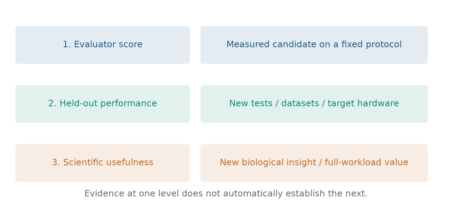
Figure 10. Original analytical framework for reading the paper’s claims. The diagram is a distinction between kinds of evidence, not an additional benchmark or a ranking of the paper’s authors.

This is why the negative results strengthen the review rather than weaken it. AC2 and MLA show that the loop does not automatically dominate strong references. Circle packing shows that matching a good construction can be a useful method check without constituting a new discovery. A paper can demonstrate a productive direction while leaving substantial room for different methods, stronger baselines, and more demanding evaluations.

14.4 The most useful follow-up measures reliability per resource

The next question is not only whether the best result improves. It is how often the improvement happens, how much evaluator work it consumes, and whether selection against noisy rewards remains stable as the budget grows. Repeated complete searches, hidden final measurements, and cost-normalized curves would answer that question more directly than another isolated headline score. They would also show where the archive’s optimistic maximum is helpful and where it amplifies noise.

These are proposed research directions, not experiments performed in this review. The paper supplies evidence that test-time learning can be useful in discovery. It leaves the broader boundary between adaptive search, metric optimization, and general scientific capability open.

15. Conclusion

TTT-Discover makes a specific and useful change to test-time computation: the system can learn from its own attempts while preserving promising candidate solutions. Adaptive entropic advantages address how strongly a good outcome should shape the policy; PUCT-inspired reuse addresses where the next attempt should begin. The resulting loop produces meaningful improvements in several continuously scored domains.

The right takeaway is conditional. When a trustworthy evaluator, reusable intermediate solutions, and enough search budget are available, learning and search can support one another. The paper does not show universal gains across all tasks, a complete total-cost advantage, or general scientific autonomy. Its strongest lesson is the design principle that the learning objective, the search memory, and the final success criterion should describe the same problem.

References and source notes

1. Mert Yuksekgonul et al. Learning to Discover at Test Time, v2, 2026-02-05. Primary source for the method, Tables 1–10, and Appendices A–F; the complete 72-page PDF was read.
2. Author project page. Resource entry and overview; numerical comparisons in this review use the selected paper version when page values differ.
3. Official project resource. Resource pointer accompanying the paper.

Equations 2, 6–7, 9’s entropy interpretation, 10, 13’s closed-form normalization, and 16 include explanatory derivations or restatements by the reviewer. All ten figures were drawn for this review. Toy distributions are labeled; table redraws cite their source table; no new empirical performance results are claimed.