AFlow: Searching for Better Agent Workflows, and Measuring What Improves

Review date: 2026-10-12
Paper: AFlow: Automating Agentic Workflow Generation
Authors: Jiayi Zhang, Jinyu Xiang, Zhaoyang Yu, Fengwei Teng, Xionghui Chen, Jiaqi Chen, Mingchen Zhuge, Xin Cheng, Sirui Hong, Jinlin Wang, Bingnan Zheng, Bang Liu, Yuyu Luo, Chenglin Wu
Identifier and version: arXiv:2410.10762v4, 2025-04-15; first submitted 2024-10-14
Resources: Full paper · Author-provided project resource

1. The useful question: who designs the process around the model?

A model can generate an answer, compare several answers, critique a draft, or write a small program that computes a result. The difficult design decision is often how these operations should be connected. Should verification precede selection or follow it? Should a failed test trigger a repair, another independent attempt, or a fallback? Should five reasoning samples be spent on every input, or only on uncertain ones? AFlow turns this layer of design into an object of search. A language model proposes changes to an executable workflow; another set of model calls supplies task-level feedback; a tree records where each change came from.

The paper’s strongest contribution is this combination of a flexible representation with locally organized experience. It does not train the weights of an executor. It searches for a reusable program around a fixed executor, using examples from a target task family. Once selected, that program can process many new inputs. This distinction is central to interpreting both its efficiency and its relevance to self-improving agent harnesses. Improvement occurs during an outer design procedure, rather than automatically after every deployed interaction.

My reading is that AFlow offers convincing evidence that workflow choice matters under its benchmark settings, but less decisive evidence that its particular tree search is the unique source of the gains. The result tables combine several ingredients: reusable operators, code-based control flow, feedback-informed prompts, repeated evaluation, and selection among candidates. A strong whole-system result is not a causal decomposition of those ingredients. The appendix also contains parameter and stopping-rule discrepancies that matter for a precise understanding of the algorithm.

Three numerical distinctions guide this review. The reported 5.7% average improvement is consistent with a relative increase from a rounded macro average of 76.0 to 80.3, a 4.3 percentage-point difference. The inexpensive configuration associated with the 4.55% headline reaches approximately the GPT-4o direct-call score; configurations that clearly exceed that score have different cost ratios. Finally, those dollar comparisons concern execution on a divided HumanEval test set, rather than the full expense of discovering the workflow. All three distinctions preserve the value of the result while narrowing what it establishes.

2. Prerequisites: programs, estimators, and two meanings of a node

A workflow is a program that maps an input to an output through several operations. An operation may call an LLM; a branch may inspect a test result; a loop may generate several candidates. The program can be fixed even when the path taken through it depends on the input. A fixed program with an if-statement is therefore different from a system that rewrites its program during inference. AFlow primarily discovers the former.

The paper describes an LLM-invoking node through a model, a temperature, a prompt, and an output format. A JSON-producing verifier and a free-text generator can use the same underlying model yet behave as different nodes. Edges describe when nodes run and which intermediate values they receive. An operator packages a familiar combination into a reusable interface: generating several solutions and choosing one, for example, saves the optimizer from expressing every detail on every proposal.

There is another meaning of node in the outer search tree. Here a node contains an entire workflow, its score, and its relationship to a parent workflow. It is not one thought, one tool call, or one step in answering a question. Confusing these levels makes AFlow look like a per-question reasoning tree. In fact, it is searching for a program that will answer a collection of questions. Figure 1 separates the levels explicitly.

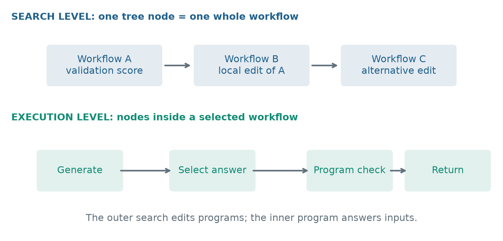
Figure 1. Original explanatory diagram based on Sections 3–4. The arrows in a search tree represent edits between workflows; the arrows inside a workflow represent execution and data flow.

Evaluation introduces a second distinction: the true quality of a workflow and its measured quality are not identical. Let an input and answer pair be drawn from a task distribution, and let the executor’s randomness be represented by a seed. A population-level objective and its empirical estimate can be written as:

$$J(W)=\mathbb{E}_{(x,y),\xi}\left[g(W(x;\xi),y)\right],\qquad \widehat J(W)=\frac{1}{mr}\sum_{i=1}^{m}\sum_{j=1}^{r}g(W(x_i;\xi_j),y_i). \tag{1}$$

Here $m$ counts evaluation examples and $r$ counts repeated runs. The function $g$ might be exact correctness, a code-test outcome, or a text-overlap score. This notation is explanatory, rather than an additional equation claimed by the paper. It makes clear that adding repeated runs reduces one source of noise without adding new independent questions. A workflow can be reliably good on a small selected validation set and still generalize poorly.

In ordinary Monte Carlo Tree Search, selection and backpropagation are often associated with visit counts, upper-confidence bounds, and sampled returns. AFlow borrows the iterative tree organization but uses a different parent-selection mechanism and stores textual edit experience. Reading the method as a specific search variant is more informative than importing standard UCT guarantees into it. Its final theory discussion does not supply the assumptions or proof needed for such a transfer.

3. What is actually searched?

The broad formulation allows changes to model choice, temperature, prompts, formats, and connectivity. The evaluated system fixes the model, temperature, and format configuration to make the search tractable, then searches prompts and code-represented relationships using a supplied operator library. This is a narrower, useful engineering choice. An unrestricted conceptual space should not be confused with the space explored by the experiments.

One convenient restatement is:

$$W=(\mathcal N,E),\quad N_i=(M_i,\tau_i,P_i,F_i),\qquad W^*\in\operatorname*{arg\,max}_{W\in\mathcal S}\widehat J(W). \tag{2}$$

First, each node specifies an LLM call contract. Second, the control program $E$ decides how calls and outputs are connected. Third, the optimizer ranks the resulting programs using validation feedback. In the practical search, the changing components are mainly the prompts, selected operators, and control program; the executor configuration stays fixed within an experiment.

Code is useful here because conditions, loops, variable reuse, and fallback behavior have a natural expression. An alternative is a graph language with explicit loop and branch constructs. Such a language can represent similar behavior and may constrain invalid candidates more effectively, but its designer must define those constructs. Code trades a broader vocabulary for a harder validity problem. Expressiveness alone does not make a proposed program correct, useful, or inexpensive.

The operator library encodes a substantial prior. Generate creates a candidate; Format adapts a response to an expected presentation; Review and Revise split criticism from correction; Ensemble chooses among candidates; Test uses executable feedback; Programmer generates and runs a computational solution. Custom provides a basic route for new prompt-driven operations. These components make good proposals more probable, but also shape which ideas the search is likely to discover first.

Consider the reported GSM8K example. Five solutions are produced, an ensemble operation selects an answer, and a Programmer operation supplies a computational check or answer. The workflow returns the program output when it passes its output condition, otherwise keeping the selected reasoning answer. The important interaction is not merely having more calls. It is deciding which intermediate result should control the final return and how to preserve a usable fallback.

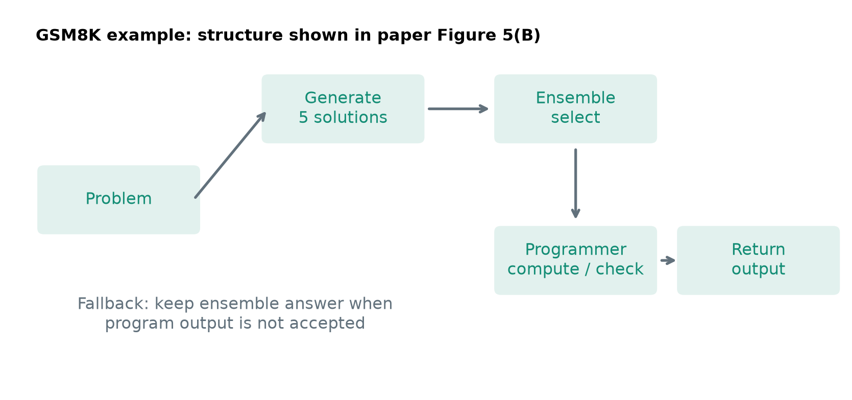
Figure 2. Original structural redraw of the paper’s Figure 5(B). It explains the stated workflow rather than reporting an independently executed system.

There is a subtle reliability boundary here. A computational result can be syntactically valid and still solve the wrong mathematical problem. A reviewer can sound confident while discarding a correct answer. A format operation can improve a metric without improving reasoning. The optimizer only knows these changes through its evaluator. Consequently, the evaluator and the data distribution are part of the effective specification of the system, not interchangeable accessories.

The paper’s optimizer prompt asks for a single modification, complete required prompts, and bounded graph complexity. That local-edit discipline makes differences easier to interpret and stores concise parent-child experience. Its downside is that some improvements require coordinated changes. Replacing an output schema without simultaneously changing consumers would be a bad edit even if the combined change were useful. A local search needs either a representation that preserves contracts or enough flexibility to propose a coherent multi-part modification under one conceptual edit.

4. The outer loop: evaluation-guided program search

AFlow splits the chosen data 20:80 into validation and test portions with seed 42. The initial template is evaluated repeatedly, and high-variance validation instances are selected for subsequent search. Each generated workflow is evaluated five times on that validation subset. The main experiments allow 20 search rounds, while the reported ADAS comparison uses 30 rounds. The test results in Table 1 average three executions of the selected workflow.

The high-variance filter has a plausible rationale: examples that sometimes succeed and sometimes fail may provide a more informative optimization signal than examples that every candidate always solves. However, this selection is based on the initial template. Later workflows can have different weaknesses. Filtering can reduce evaluation cost while also shifting the optimization target toward the initial model’s borderline cases. The complete original test partition remains important for assessing whether gains survive that shift.

Algorithm 1. AFlow’s outer search, stated at the method level

Input: task examples D, evaluator G, initial workflow W0,
       operator library O, optimizer model, executor model
1. Split D into validation V and held-out test T (20:80).
2. Evaluate W0 repeatedly; retain high-variance cases in V.
3. Initialize the workflow tree and parent-specific experience.
4. For each search round, up to the stated budget of 20:
   a. Select a parent using the mixed probability rule.
   b. Load its workflow, edit history, and execution feedback.
   c. Ask the optimizer for a coherent local workflow edit.
   d. Evaluate the child five times on V.
   e. Store the mean score, cost, edit, and parent comparison.
   f. Update the best candidate and the stopping statistic.
   g. Stop when the chosen early-stopping rule is satisfied.
5. Freeze the selected workflow; evaluate it on T.
Output: selected workflow and its validation/test measurements

This pseudocode summarizes the paper, without silently resolving its internal discrepancies. The main text retains the initial workflow among selectable parents; the appendix’s selection procedure only explicitly slices the top three recorded results. Likewise, the main text describes no improvement in a top-k average, while the appendix describes unchanged top-k workflow identities for five rounds. Those are not equivalent conditions. Three workflows can exchange small improvements while keeping the same membership, or replace each other while leaving their average effectively unchanged.

An early-stopping condition reduces wasted evaluation when a search appears stagnant. It does not prove that useful edits no longer exist. For a stochastic optimizer, five unsuccessful rounds may mean an exhausted local neighborhood, noisy evaluation, or simply an unlucky sequence of proposals. The appropriate interpretation is a budget heuristic, whose operating behavior depends on the proposal model and parent-selection distribution.

The optimizer receives more than a scalar score. It sees the selected workflow, modifications tried around it, their improvement or failure, and execution logs containing predictions and expected answers. This can turn an uninformative instruction such as “improve the score” into a concrete hypothesis: preserve a programmatic computation, repair a final-answer format, or avoid a reviewer that repeatedly overwrites correct answers. The tree organizes which experience applies to which parent, rather than treating every historical program as equally relevant context.

5. Deriving the mixed parent-selection rule

Suppose there are $n$ eligible workflows with scores $s_1,\ldots,s_n$. AFlow combines a uniform component with a score-sensitive component. Start with a softmax distribution:

$$w_i=\exp\!\left(\alpha(s_i-s_{\max})\right),\qquad q_i=\frac{w_i}{\sum_{j=1}^{n}w_j}. \tag{3}$$

Subtracting the maximum does not change relative weights: the common factor $\exp(-\alpha s_{\max})$ cancels between numerator and denominator. It keeps exponentials at most one for nonnegative $\alpha$, improving numerical stability. It does not change the units of the scores. A score expressed as 80 rather than 0.80 still changes the exponent by a factor of one hundred.

Mix this score distribution with the uniform distribution:

$$p_i=\frac{\lambda}{n}+(1-\lambda)q_i,\qquad \sum_i p_i=1,\qquad p_i\geq\frac{\lambda}{n}. \tag{4}$$

The normalization follows by adding $n$ copies of $\lambda/n$ and the normalized softmax mass. The lower bound gives every eligible parent a minimum chance of being revisited. It says nothing about workflows excluded before sampling. In particular, a top-k prefilter can remove almost all historical candidates; the uniform component does not restore exploration across that full history.

At $\lambda=1$, scores are ignored. At $\lambda=0$, the sampler is pure softmax. When $\alpha$ approaches zero, all softmax weights approach one and both mixture components become uniform. A large $\alpha$ concentrates most score-driven mass on the best eligible parent, while retaining the uniform floor. This is a practical mechanism for balancing exploitation and revisitation, not a conventional confidence-bound rule based on uncertainty or visit count.

Algorithm 2. Stable mixed sampling with explicit score units

Input: eligible parent list C, score vector s, lambda, alpha
1. Confirm that every score uses the same documented units.
2. Set n = length(C) and b = maximum(s).
3. For each i, compute w[i] = exp(alpha * (s[i] - b)).
4. Normalize q[i] = w[i] / sum(w).
5. Set p[i] = lambda/n + (1-lambda) * q[i].
6. Sample one parent from the categorical distribution p.
Output: sampled parent and the probability vector

A concrete example exposes why units matter. With scores 0.70, 0.75, and 0.80, the main-text parameters yield probabilities very close to one third each. Expressing the same performances as 70, 75, and 80 produces much stronger concentration on the best parent. Figure 3 evaluates the formula directly; these are analytical illustrations, not measurements from an AFlow run.

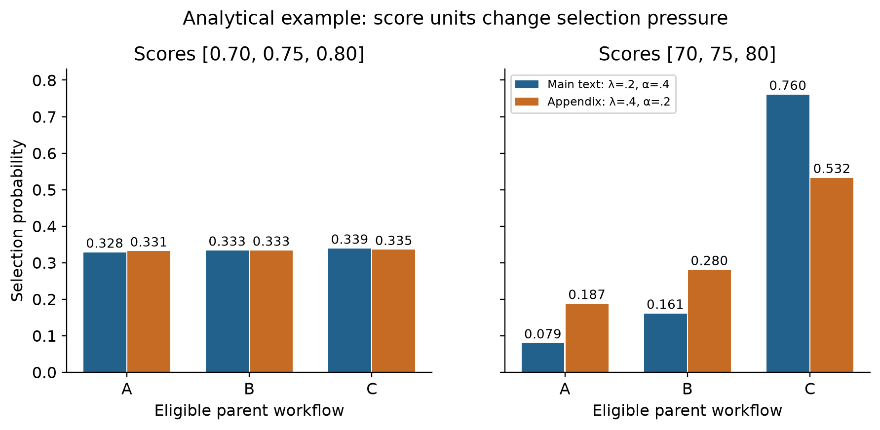
Figure 3. Original calculation of the published mixture formula. Section 4 specifies lambda 0.2 and alpha 0.4; Appendix A.6 reverses those values. The figure does not choose an undocumented authoritative setting.

The discrepancy is material because both the uniform fraction and the score temperature change. The appendix’s example experience scores are fractions, whereas experiment tables often display percentages. A careful methodological description should preserve this ambiguity instead of presenting a guessed configuration as settled. Importantly, none of this invalidates the reported benchmark table by itself; it limits the precision with which the described search can be reconstructed from the paper alone.

For fixed scores, the odds in the softmax component satisfy:

$$\frac{q_i}{q_j}=\exp\!\left(\alpha(s_i-s_j)\right). \tag{5}$$

This relation makes the sensitivity transparent. Doubling a score gap has the same effect as doubling $\alpha$. Rescaling scores without compensating $\alpha$ changes the algorithm. A rank-based selector would avoid that dependence but discard information about how large improvements are. An uncertainty-aware selector would use repeated-run variation, but would need a justified model for noisy and adaptively chosen measurements. AFlow’s simpler mixture is easy to calculate, while leaving those alternatives open.

6. Repeated evaluation: useful averaging, incomplete uncertainty control

For one candidate, let $z_j$ be its aggregate validation score in repeated run $j$. The paper computes a mean and standard deviation from five runs. The familiar estimators are:

$$\bar z=\frac{1}{r}\sum_{j=1}^{r}z_j,\qquad \widehat\sigma^2=\frac{1}{r-1}\sum_{j=1}^{r}(z_j-\bar z)^2, \qquad r=5. \tag{6}$$

If runs were independent samples from a stationary execution process, the standard error of the mean would be approximately $\widehat\sigma/\sqrt r$. That condition is useful but incomplete. Repeating the same questions cannot reveal all uncertainty about future questions. Shared API behavior, correlated candidate answers, and adaptive selection can also weaken a naive interpretation of five runs as five fully independent measurements.

The comparison between a child and its parent is especially important. A child is marked successful relative to its parent’s measured performance. A tiny positive difference may be noise. If per-example outcomes are available under comparable conditions, a paired difference focuses on changes on the same examples:

$$d_i=g(W_c(x_i),y_i)-g(W_p(x_i),y_i),\qquad \widehat\Delta=\frac{1}{m}\sum_{i=1}^{m}d_i. \tag{7}$$

This is a proposed analytical extension, not an additional procedure reported in AFlow. It helps distinguish a workflow that improves difficult examples consistently from one whose aggregate mean happens to rise. For deployment decisions, reporting a paired interval across examples and repeating the whole search would answer different questions: uncertainty about the chosen workflow and uncertainty about the search procedure that chose it.

There is also selection bias. Searching many candidates and choosing the highest noisy estimate tends to select positive noise along with real quality. If $\widehat J_i=J_i+\epsilon_i$, the winner’s noise is generally not distributed like the noise of a candidate selected in advance. More search can improve true quality while widening the gap between the best validation measurement and future performance. This is why the held-out test partition must remain outside the optimizer’s feedback loop.

The high-variance subset makes the budget attractive but deserves a distributional interpretation. Suppose a deployment workload contains easy formatting tasks, arithmetic tasks, and rare cases requiring a different strategy. A subset chosen by instability of a simple initial workflow may disproportionately represent one category. The optimizer can then specialize to that category. The remedy is not necessarily to evaluate every candidate on every example, but to reserve an independent selection or confirmation sample and document how validation examples were chosen.

7. Reading the six-benchmark evidence

The main table uses GPT-4o-mini as executor for every compared method. The optimizer is Claude 3.5 Sonnet. The tasks span text question answering, program generation, and mathematical reasoning. The metrics are not all the same: HotpotQA and DROP use F1, HumanEval and MBPP use pass@1, and GSM8K and MATH use solve rate. Their macro average is an equal-weight summary of six score columns, not an accuracy over a pooled collection of questions.

The data selection is also specific. The paper uses the full selected datasets for GSM8K, HumanEval, and MBPP, before its validation/test division; HotpotQA and DROP use 1,000 randomly selected examples each. MATH uses 617 level-5 problems from four categories: counting and probability, number theory, prealgebra, and precalculus. Thus the MATH column should not be read as a result on every problem in the original MATH benchmark. These choices matter when comparing a number with results from another paper.

Dataset	Direct IO	CoT self-consistency	ADAS	AFlow
HotpotQA	68.1	68.9	64.5	73.5
DROP	68.3	78.8	76.6	80.6
HumanEval	87.0	91.6	82.4	94.7
MBPP	71.8	73.6	53.4	83.4
GSM8K	92.7	92.7	90.8	93.5
MATH subset	48.6	50.4	35.4	56.2

These numbers are transcribed from Table 1. The self-consistency baseline generates five answers; the paper also includes CoT, MedPrompt, MultiPersona, and Self Refine. AFlow leads every dataset column in that table. Figure 4 gives the same comparison a visual scale so that the relatively small GSM8K gain is not mistaken for a uniform effect across tasks.

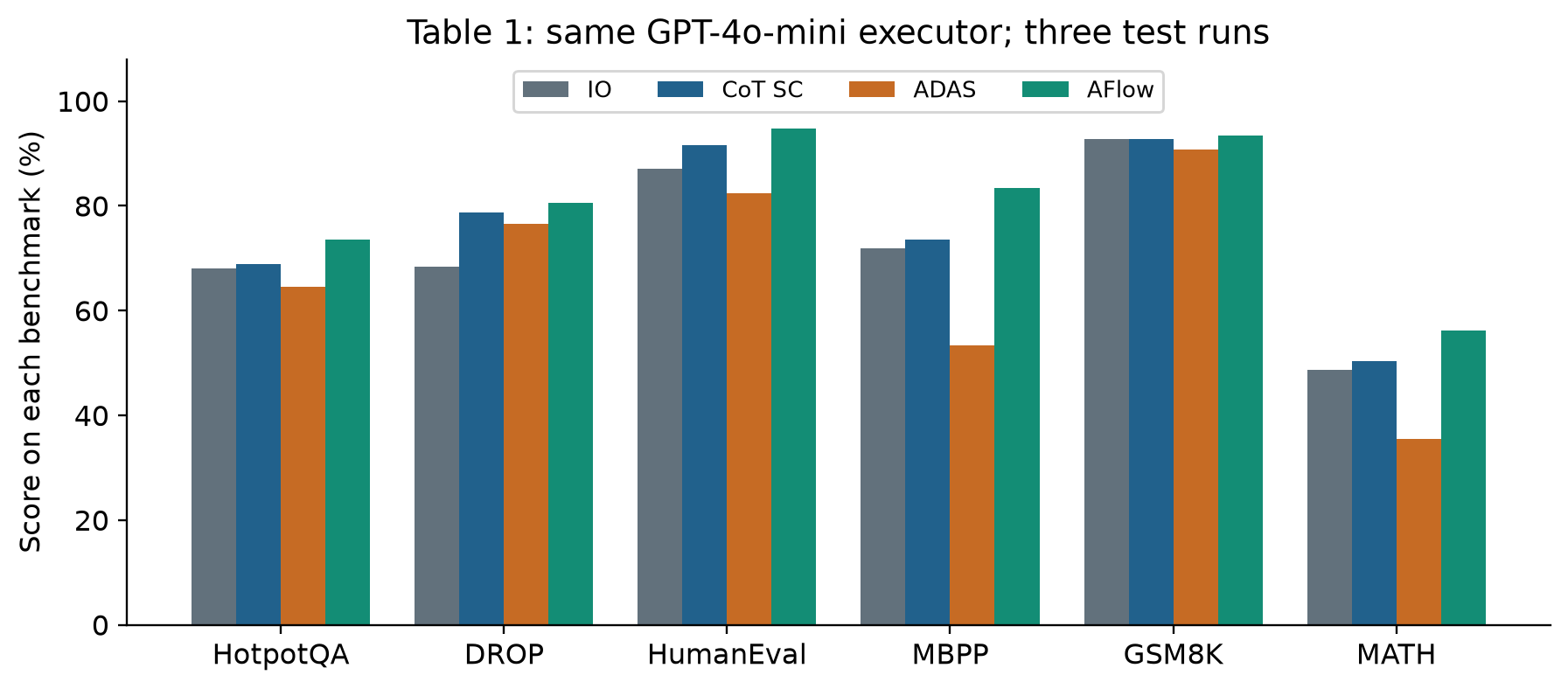
Figure 4. Original plot of reported Table 1 values. Scores share a percentage display but use different task metrics; no new model experiment was performed.

Using the paper’s rounded macro averages, the headline comparison is:

$$\Delta_{\mathrm{pp}}=80.3-76.0=4.3,\qquad \Delta_{\mathrm{relative}}=\frac{80.3-76.0}{76.0}\times100\%\approx5.66\%. \tag{8}$$

Against the ADAS macro average of 67.2, the analogous difference is 13.1 points or approximately 19.49% relative. Neither is an absolute improvement of 19.5 percentage points. Reporting the baseline, numerator, and denominator avoids a common ambiguity in summaries of agent benchmarks.

A different comparison takes the best manual method separately for each dataset. The respective manual maxima are 69.2, 78.8, 91.6, 73.6, 92.8, and 50.8. AFlow’s gains over those maxima are 4.3, 1.8, 3.1, 9.8, 0.7, and 5.4 points. This is an oracle-like combination of different baselines, rather than one executable competing system, but it reveals where the improvement is concentrated. MBPP contributes much more than GSM8K.

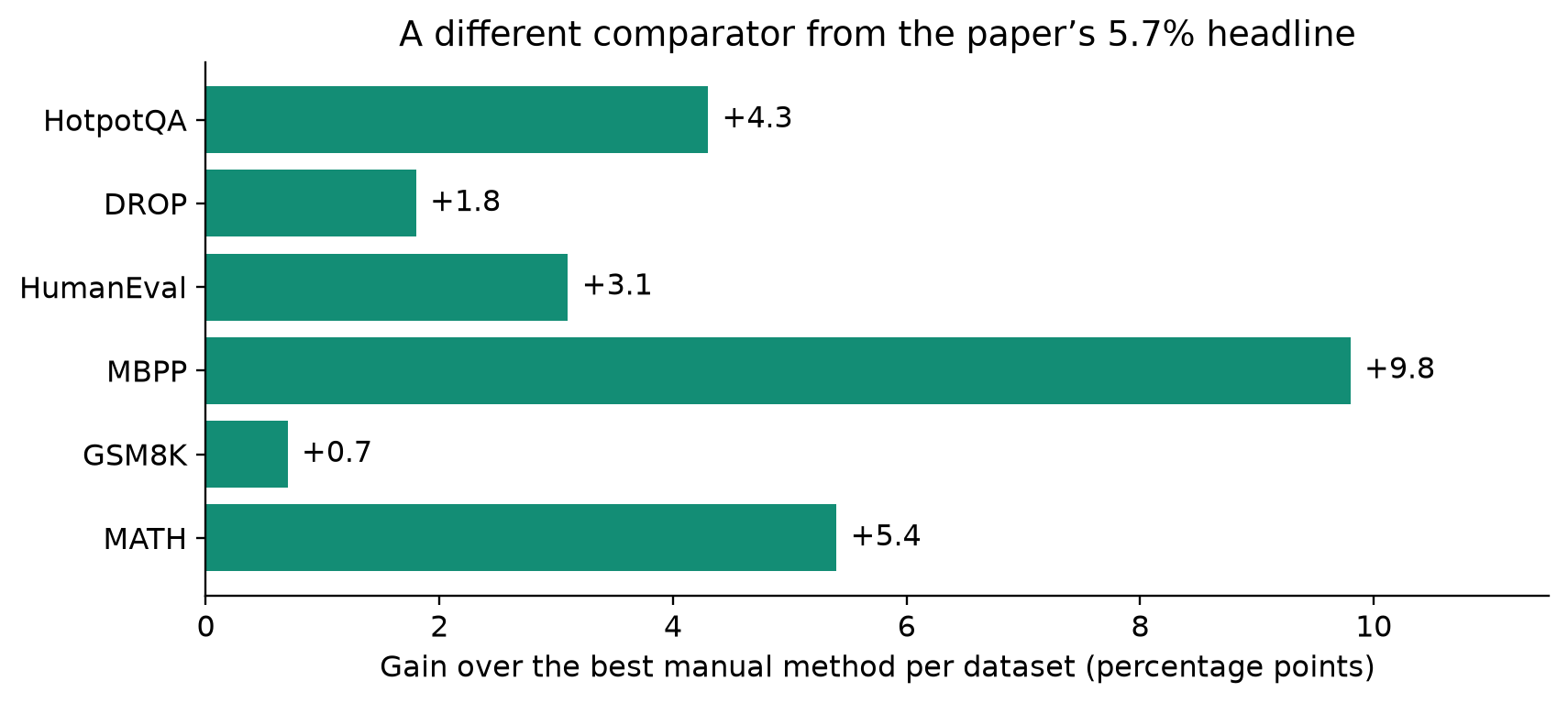
Figure 5. Original subtraction from Table 1. Choosing a different manual baseline for each dataset answers a different question from comparing two macro-average rows.

For code generation, pass@1 describes the final returned answer of a workflow. It does not imply the workflow made only one LLM call or produced only one internal candidate. A three-candidate ensemble with tests can still return one final program evaluated under pass@1. This is a legitimate system comparison, provided its additional computation is visible. It is not a claim that the base model’s single raw sample acquired the same quality.

The Test operator’s information budget deserves attention. Appendix A.4 uses public tests; for MBPP it treats the first test case of each problem as public under its stated setting. This provides a useful feedback channel. A comparison with a system that cannot access such examples would conflate workflow quality with feedback availability. The reported setting should therefore travel with the result, especially when discussing test-driven correction as a source of improvement.

8. Transfer: the program travels, but its quality is model-dependent

Table 2 evaluates HumanEval workflows found using two different executors. One search uses GPT-4o-mini; the other uses DeepSeek-V2.5. The resulting workflows are then executed with four model families/configurations. Most transferred workflows beat the corresponding direct-call baseline, supporting the idea that some useful structure is reusable across executors.

The pattern also shows specialization. GPT-4o-mini scores 94.7 with its own searched workflow but 90.8 with the DeepSeek-derived workflow. DeepSeek-V2.5 scores 94.7 with its own workflow and 93.9 with the mini-derived one. GPT-4o reaches 96.2 with the mini-derived workflow, compared with 93.9 under direct IO. These are rounded Table 2 values, and the appendix gives some more precise scores.

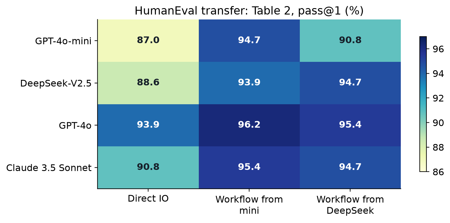
Figure 6. Selected Table 2 columns, redrawn as a heat map. Each row holds the execution model fixed; columns change the workflow’s origin.

Transfer is therefore a graded property. A workflow can remain useful after a model swap without remaining optimal. Different models may benefit from different prompt styles, error-correction frequency, output formats, and candidate diversity. A weaker model may need a more explicit computational route, while a stronger one may be harmed by an unnecessary revision step. The table supports retesting a workflow after changing its executor, rather than assuming an abstract graph has model-independent value.

The evidence is also limited to the tested transfer setting. Cross-model HumanEval transfer is not the same as transfer from code generation to scientific research, or from benchmark questions to a long-running application with persistent state. The program representation makes those extensions conceivable, but the reported table does not measure them. AFlow is a useful starting point for harness design because the unit being optimized is reusable, not because it has demonstrated universal reuse.

9. Cost: a precise reading of the inexpensive-workflow claim

Appendix D reports historical dollar costs for executing the divided HumanEval test set. It supplies enough values to separate three comparisons against GPT-4o IO, whose listed score is 0.9389 and cost is $0.6371. DeepSeek executing the mini-derived workflow scores 0.9390 at $0.0291. At the displayed precision this is essentially parity, and the paper’s detailed text calls it parity. The approximately 4.55% figure should not be attached to a substantial quality improvement.

DeepSeek executing its own searched workflow scores 0.9466 at $0.0377. GPT-4o-mini executing its own workflow scores 0.9470 at $0.0513. These configurations exceed the displayed GPT-4o IO score, with different cost ratios. Using the rounded values printed in the appendix:

$$\begin{aligned} 100\frac{0.0291}{0.6371}&\approx4.57\% &&\text{near parity},\\ 100\frac{0.0377}{0.6371}&\approx5.92\% &&\text{higher displayed score},\\ 100\frac{0.0513}{0.6371}&\approx8.05\% &&\text{higher displayed score}. \end{aligned} \tag{9}$$

The small difference between 4.57% computed here and 4.55% reported in the paper can arise from rounding or a different underlying precision; the displayed table alone does not resolve it. The more important issue is identifying which score and which workflow go with each ratio. Nor does a 0.0001 displayed score difference establish a statistically meaningful improvement.

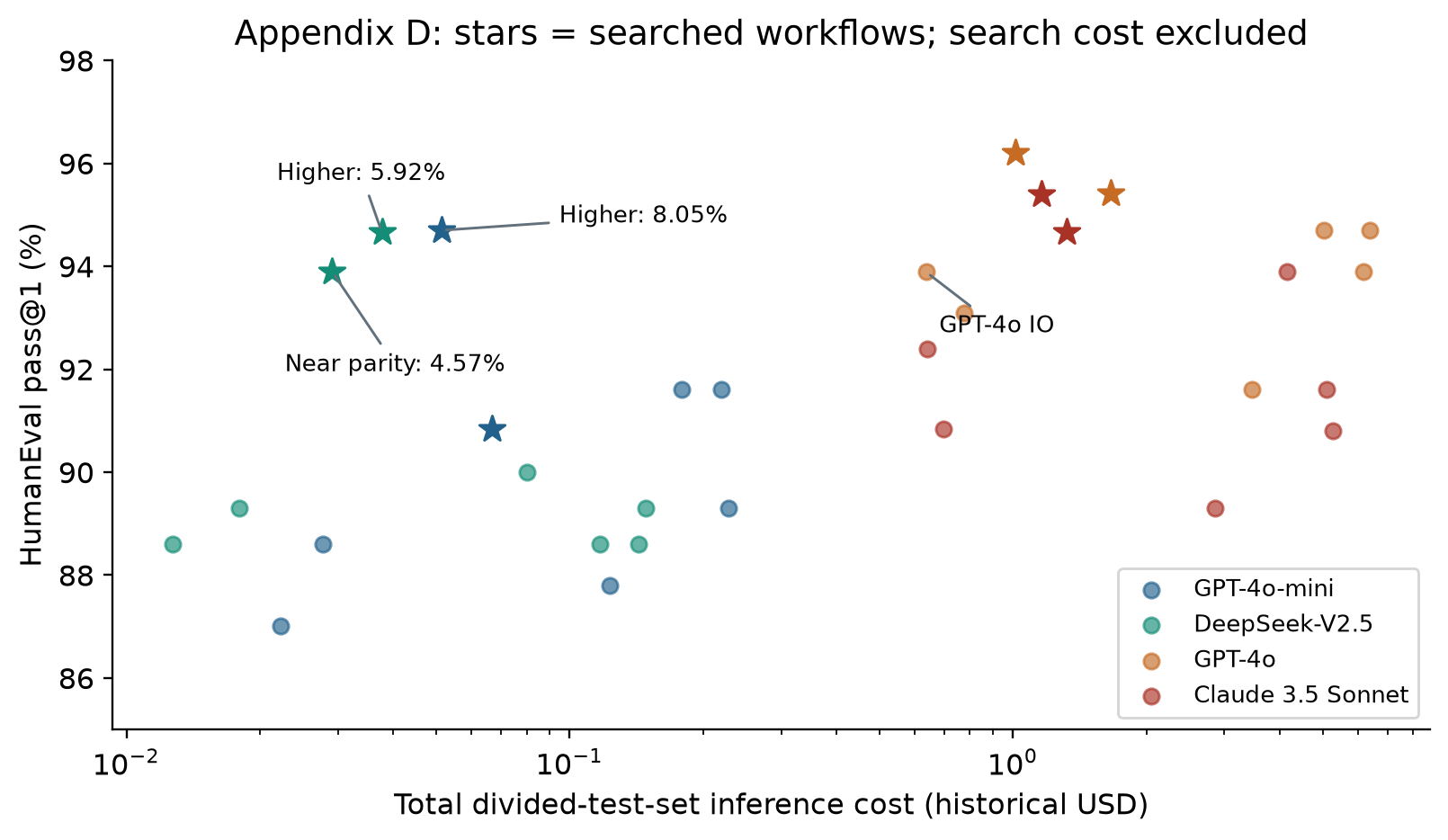
Figure 7. Original plot of all 32 Appendix D model/method entries. Stars denote searched workflows. The x-axis is the test-set execution cost, excludes search, and does not represent current API prices.

Search has a separate expense. It includes optimizer calls, repeated candidate evaluation, the initial filtering runs, and any failed proposals. If the selected workflow is reused many times, that expense can be amortized. Let $S$ be its search cost, $c_A$ its inference cost per comparable future batch, and $c_B$ the alternative’s cost. Then:

$$C_A(B)=S+Bc_A,\qquad C_B(B)=Bc_B,\qquad B>\frac{S}{c_B-c_A}\quad(c_B>c_A). \tag{10}$$

This follows by moving the recurring-cost terms to one side of $S+Bc_A<Bc_B$. The unit of $B$ must match the unit of the reported cost. Here a batch means a workload the size of the divided test set; it is not one question. With $c_A=0.0513$ and $c_B=0.6371$, every additional comparable batch saves $0.5858 before search cost. A hypothetical $10 search would break even after more than 17.07 such batches. The paper does not establish that $10 is the actual search expense.

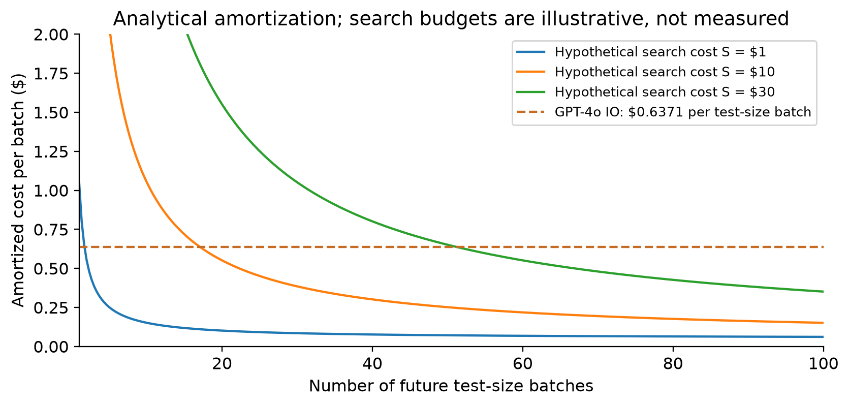
Figure 8. Analytical illustration using Appendix D execution costs and explicitly hypothetical search budgets. It shows the dependence on reuse volume, not a measured return on investment.

Dollar cost is also only one resource dimension. Five serial calls may be cheap but too slow for an interactive application. Parallel candidates can shorten some latency at the cost of concurrent capacity. A workflow that fixes more errors may still have a long-tail timeout problem. The paper’s cost-quality frontier is useful for its defined accounting boundary, while leaving latency, wall-clock search time, and operational reliability as separate questions.

Algorithm 3. Interpreting a workflow’s economic case

Input: measured search expense S, batch costs cA and cB,
       quality estimates, expected deployment volume B
1. Confirm that cA and cB cover the same amount of work.
2. Compare quality with uncertainty, not rounded scores alone.
3. Calculate recurring savings d = cB - cA.
4. If d <= 0, there is no cost-only amortization threshold.
5. Otherwise calculate the threshold Bstar = S / d.
6. Compare expected B with Bstar; add latency and failure costs.
7. Recalculate after a model, pricing, or workload change.
Output: a conditional deployment argument, not a universal claim

This third algorithm is the review’s proposed decision procedure. It is deliberately separate from AFlow’s search algorithm: the optimized validation score does not by itself decide whether deploying the winner is worthwhile.

10. What the search trajectories actually teach

The GSM8K case progresses from a simple initial workflow through an ensemble step, a Programmer step, and prompt changes. The figure reports improvements along a successful path, but also shows branches that do not help. A review step that changes a developed answer without sufficient additional reasoning can lower accuracy. A prompt revision emphasizing discount information can over-specialize. The lesson is that an intuitively sensible operation must still earn its place through task feedback.

Appendix C gives a more detailed MATH experience tree. A selected successful path rises from approximately 0.4874 to 0.5244, then 0.5277, then 0.5513. The associated changes include a programmatic solution, ensemble selection, and a detailed reasoning candidate. Yet near the same parent, several modifications described in similar terms receive very different scores. Adding an ensemble is not an intervention with one stable effect independent of its inputs and neighboring operations.

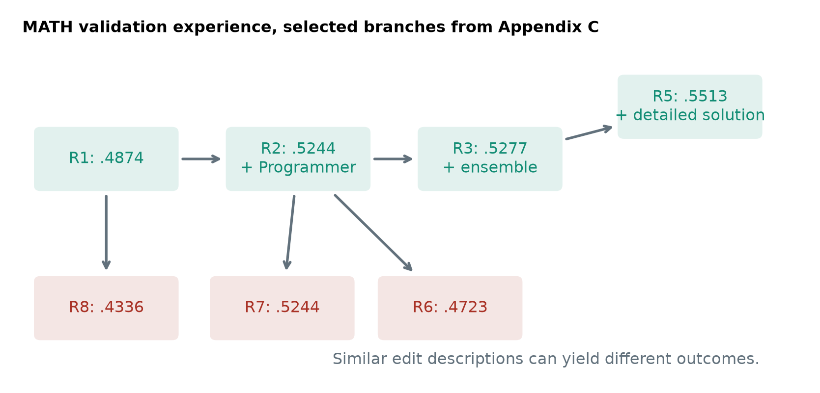
Figure 9. Original diagram of selected Appendix C validation records. Rounded scores belong to the search trajectory and should not be substituted for held-out test results.

This is where parent-specific experience becomes useful. A modification has a context: what information was available, what output was expected, which operator produced it, and where failures occurred. Storing “ensemble helped” globally is weaker than storing “this change helped this parent on these examples.” The tree can preserve such local evidence while keeping unsuccessful proposals available as negative examples.

At the same time, these examples are explanatory cases. A successful trajectory cannot tell us how often another search seed would find a similar result. Nor does labeling a branch as a failure imply its idea can never work. A branch can lose because of a poor prompt, an unsuitable input representation, a brittle output condition, or measurement noise. Interpretable edit records are valuable precisely because a scalar score collapses these different possibilities.

The appendix’s narrative and its stored edit descriptions are not always perfectly aligned. For example, the discussion of the round-1-to-round-8 MATH change invokes loss of programmatic capability, while the displayed experience summarizes an ensemble addition. That is a reason to avoid treating brief natural-language edit labels as a complete causal account. This review uses the numerical record to describe outcomes and treats the accompanying explanation as the authors’ interpretation.

The operator ablation on GSM8K reports 93.1% without predefined operators, and the main AFlow result is 93.5%. The ablated method can construct an ensemble-like pattern using Custom calls, indicating that the representation and optimizer still contain useful prior knowledge even after the explicit library is removed. “No operators” does not mean no knowledge of workflow patterns: the optimizer’s pretrained capabilities and the surrounding instructions remain.

The ablation is therefore best read as evidence that packaged operators improve search efficiency and can help final quality in this setting, rather than proof that operator priors are unnecessary in all domains. Removing a library also changes proposal difficulty and validity. A matched-budget comparison would need to account for how many evaluable candidates are actually produced and how much evaluation cost is spent before comparing final scores.

11. Open-ended tasks: feedback is still the bottleneck

Appendix F extends the method to a novel-writing prompt and ten academic-idea prompts. GPT-4o supplies a four-dimension judgment, each dimension scored from one to five, with a total of twenty. The dimensions cover relevance, content quality, coherence, and comparison with an expected or reference answer. Three human annotators also score outputs. This is useful preliminary evidence that the outer loop can operate when an exact symbolic checker is unavailable.

The results should nevertheless be separated from the six-benchmark evaluation. The novel case uses one prompt. The paper reports a final output of about 27,000 words even though the requested length was exactly 20,000. That is an approximately 35% overshoot, not exact satisfaction of the length requirement. A high overall quality score can coexist with failure on a concrete constraint. This is a particularly clear example of why an aggregate reward may not fully represent the task.

The idea-generation table shows LLM and human scores moving in broadly similar directions, but with different magnitudes. At round four, the LLM score is 17.6 while the human average is 9.7. Selecting candidates against one judge can exploit that judge’s tolerance for weaknesses that another evaluator notices. Correlation in final rankings is encouraging; disagreement on intermediate candidates shows why independent assessment remains informative.

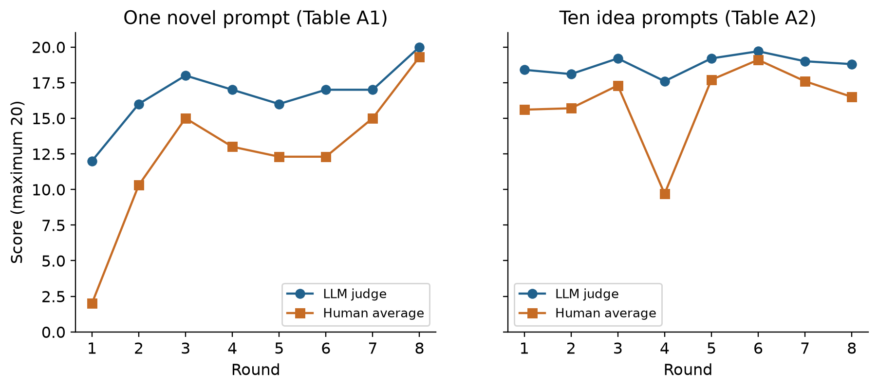
Figure 10. Original plots of Tables A1 and A2. The novel panel concerns one prompt and the idea panel ten prompts; the two settings do not constitute a broad open-ended-task benchmark.

A helpful formal distinction is between the judge reward $R$ and the actual user utility $U$. Search optimizes the first, while deployment cares about the second. An illustrative decomposition is:

$$R(W)=U(W)+b(W)+\epsilon(W). \tag{11}$$

Here $b(W)$ represents systematic evaluator bias and $\epsilon(W)$ measurement noise. Repeated judging can reduce some noise but will not eliminate a consistent preference for verbosity, familiar structure, or superficial compliance. If search can increase the bias term more cheaply than utility, it can produce a better judge score without a better user outcome. This is an analytical model of the risk, not a fitted model of AFlow’s experiments.

For a task with a hard constraint, a more faithful selection rule might maximize a quality score only among feasible outputs. For example, a word-count tolerance can be measured separately from narrative quality. The lesson from the novel case is not that automatic workflow generation cannot help long-form writing. It is that the evaluator must distinguish an improvement in the product from successful completion of the whole request.

12. Limitations and failure boundaries

The target is a task-family workflow. The main evidence concerns bounded QA, coding, and mathematics benchmarks with evaluable outputs. Persistent memory, changing tools, irreversible side effects, and tasks lasting days introduce different state-management problems. AFlow’s flexible program representation can express mechanisms for those problems, but expression is not evidence of successful adaptation.

The comparison isolates executor identity more clearly than total compute. Holding GPT-4o-mini fixed is helpful, but candidate count, operator access, optimizer effort, and inference calls differ between methods. Twenty AFlow rounds and thirty ADAS rounds are different search budgets, and equal round counts would not necessarily imply equal token or dollar costs. The results support a system-level improvement under the stated configuration, with a less complete accounting of which ingredient contributes how much.

The evaluator is part of the learned behavior. Formatting corrections may remove unfair penalties for correct answers, which is a real benefit. They can also dominate the reward signal or encourage output patterns fitted to one scoring rule. Public-test feedback is useful for repairing programs, but it makes test availability a condition of the result. Judge-based extensions bring their own systematic biases.

Parameter and procedure descriptions need reconciliation. The main text and Appendix A.6 disagree on lambda/alpha values, explicitly including the initial parent, and the early-stopping definition. The appendix also labels the 80% split as training in one algorithm comment, while the experimental setup identifies it as test. This review follows the experimental description for the data split and preserves the other discrepancies as unresolved paper-level details.

Finite search is not a global-optimality certificate. Appendix G argues from bounded evaluation, valid code, and nonzero chances of improvement. Those conditions alone do not establish that twenty rounds, or any fixed finite number, must discover an optimum. A bounded score is not a finite search space. A nonzero probability can be arbitrarily small, and a sequence of improvements need not reach the global best program.

To see the distinction, assume an idealized, independent probability $p$ of finding a particular useful candidate in each round. Then:

$$\Pr(\text{found by }N)=1-(1-p)^N. \tag{12}$$

For $p=0.01$ and $N=20$, this probability is only about 18.2%. Even in this much simpler model, “nonzero chance” does not imply a finite-budget guarantee. Real search is more complicated because eligible parents change, proposals depend on experience, and some useful workflows require multiple edits. The formula is a counterexample to an over-strong inference, not an estimate of AFlow’s success rate.

13. Critical analysis: where the next convincing evidence would come from

The most compelling interpretation of AFlow is that it makes feedback-guided workflow design concrete. It specifies a program representation, a manageable parent pool, a proposal mechanism, a repeated evaluator, and a memory organized by edit ancestry. This combination turns vague self-improvement into a sequence of inspectable decisions. The strongest scientific question remaining is how much each decision rule matters when budgets and evaluation opportunities are held comparable.

First, tree memory and candidate selection should be separated experimentally. A linear search with the same operator library, the same edit prompt, and the same amount of relevant parent-local feedback would be more informative than comparing two systems with several simultaneous differences. Conversely, a tree-shaped archive with random parent selection could test how much the score mixture contributes. These are proposed studies; the paper’s current tables do not provide their outcomes.

Second, the objective can be broadened from raw score to a constrained quality-cost trade-off. A useful formulation would be:

$$\max_W J(W)\quad\text{subject to}\quad \mathbb E[C(W)]\leq c_{\max},\quad \Pr(L(W)>\ell_{\max})\leq\delta. \tag{13}$$

The first constraint limits average expense; the second limits the chance of excessive latency. This is a review proposal, not the implemented objective claimed in the paper. It captures why a workflow with the highest validation mean may not be the best deployed system. A bounded retry, a reliable fallback, or a smaller candidate ensemble can be preferable when latency and failure costs matter.

Third, evaluation should distinguish discovering a good workflow once from reliably discovering one. Repeating the whole outer search with different seeds and reporting the distribution of held-out scores would reveal sensitivity to initial validation selection and optimizer sampling. Publishing every search’s cost-quality endpoint would also make the practical trade-off clearer than showing only the strongest discovered workflows. Confidence intervals over final execution alone cannot answer this search-level question.

Fourth, the relationship between local explanations and causal evidence should stay explicit. A parent-child comparison is informative, but the edit can change several details, and the measured score is noisy. Claims such as “ensemble improved reasoning” need more support than a label on one successful edge. The paper’s own failed ensemble branches show that behavior depends on context. That is precisely why retaining failed trials is useful for design, while not turning them into universal laws.

Finally, the harness perspective suggests a boundary between proposal and retention. An optimizer may invent a promising workflow for one family of tasks. Retaining that workflow for future use requires separate evidence that it preserves contracts, helps on unseen examples, and does not merely exploit the current evaluator. AFlow provides an outer search and useful local experience; a general self-evolving system would additionally need policies for compatibility, retirement, and independent-task reuse. This is a natural extension of the paper’s design, rather than an ability already demonstrated by its benchmark results.

My overall judgment is positive with a specific scope. The empirical tables make a strong case for searching the procedure surrounding a model. The interpretability of the search history and the portability of executable workflows are particularly useful ideas. The paper is less conclusive about global convergence, general-purpose autonomy, and total economic savings after discovery. Keeping those claims separate makes the work more actionable, because it identifies exactly which measurements a follow-up study should add.

14. Conclusion

AFlow treats an agentic workflow as a program that can be improved through execution feedback. Its outer search selects whole workflows, proposes local changes, evaluates them repeatedly, and stores what happened near each parent. In the reported six-benchmark setting, the resulting systems consistently improve over the compared baselines with the same GPT-4o-mini executor.

The details determine the interpretation: a 5.7% relative macro gain is not a 5.7-point gain; a cheap near-parity configuration is different from a higher-scoring configuration; and low inference expense does not erase search cost. The parameter discrepancies, score-scale sensitivity, and open-ended constraint failure are useful reminders that automatic optimization inherits the specification supplied by its evaluator. The transferable lesson is to search reusable behavior while measuring quality, cost, and generalization at the level where the behavior will actually be used.

References and figure provenance

1. Zhang et al. AFlow: Automating Agentic Workflow Generation, v4. Methods: Sections 3–4 and Appendix A; benchmark results: Section 5, Tables 1–2; detailed cost values: Appendix D; case studies: Appendices B–C and F; theoretical discussion: Appendix G. All 38 PDF pages were read for this review.
2. Versioned source PDF. The ten figures in this review are newly drawn explanations, plots of the paper’s reported numerical facts, or explicitly labeled analytical illustrations. No newly reproduced model results are claimed.
3. Author-provided AFlow resource. Resource entry for readers interested in the project.

Equation numbering and the three pseudocode algorithms belong to this review. Algorithms 1–2 explain the paper’s method while preserving stated ambiguities; Algorithm 3 and Equations 7, 10–13 provide independent interpretation and proposed evaluation criteria. Dollar amounts are historical values in the source paper.