SAES-SVD: Compensating for the Errors That Earlier Layers Leave Behind

Review date: October 9, 2026
Review author: Zhongzhu Zhou
Paper reviewed: SAES-SVD: Self-Adaptive Suppression of Accumulated and Local Errors for SVD-based LLM Compression
Paper authors: Xing Hu, Dawei Yang, Yuan Cheng, Zhixuan Chen, Zukang Xu
Paper version: arXiv:2602.03051v1, February 3, 2026

1. The input to a compressed layer has already changed

I find the most useful entry point to SAES-SVD to be a distinction between two reconstruction targets. Suppose an early transformer block has been compressed. A later linear layer now receives a different activation matrix. Should its low-rank replacement imitate the original weight on this changed input, or imitate the output that the uncompressed network would have produced? These targets are generally different. A method can be excellent at the first task while the whole network drifts away from its reference trajectory.

SAES-SVD makes that distinction explicit. Its Cumulative Error-Aware Layer Compression, or CEALC, combines local reconstruction with alignment to the full-precision path. Its Adaptive Collaborative Error Suppression, or ACES, chooses the alignment coefficient using a spectral surrogate. The central mathematical result is a low-rank regression problem reducible to an SVD after whitening. The coefficient search is a separate approximation; it is not the same theorem and does not inherit a guarantee of optimal language-model quality.

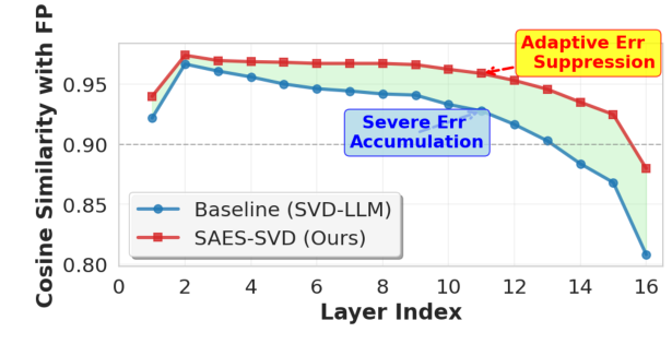
Figure 1 (paper Fig. 1a): output similarity across depth motivates cumulative-error compensation. Cropped from Hu et al., CC BY 4.0. The figure caption names LLaMA-3-8B, while nearby prose names LLaMA2-7B; I treat the plot as qualitative motivation rather than resolving that discrepancy by assumption.

The method is attractive because it changes the compression target rather than requiring a new inference operator. At serving time the result is still a pair of dense low-rank factors. During compression, however, it needs paired activations from the compressed and original paths. That makes calibration quality, reference alignment and the order of layer replacement central to the argument.

This review covers all 26 pages of v1, including the proofs, extra experiments and algorithms in Appendix A. Equations and numbered procedures below are explanatory reconstructions of the paper. Small matrix examples are analytical illustrations, and experimental values are attributed to the original tables. I did not run model-compression experiments. Several statements in the paper disagree with its tables or algorithm listing; I retain the disagreements where they affect interpretation instead of silently choosing the more favorable number.

2. Prerequisites: three meanings of low-rank error

Let $W\in\mathbb{R}^{m\times n}$ be a linear weight, $X\in\mathbb{R}^{n\times N}$ a matrix of calibration activations, and $U=AB$ its rank-at-most-$r$ replacement. The factors have shapes $m\times r$ and $r\times n$. Their parameter count is $r(m+n)$, compared with $mn$ for the dense matrix. Ignoring biases and metadata, a parameter reduction requires

$$r(m+n)<mn,\qquad r<\frac{mn}{m+n}. \tag{1}$$

For a square matrix, rank below the original dimension is not enough: it must be below half that dimension to reduce the number of stored scalars. At $m=n=4096$, a factorization with $r=2048$ has exactly as many scalars as the original. This is a simple but important distinction between mathematical rank reduction and practical compression. Whole-model ratios also depend on embeddings, norms, untouched layers and factor precision.

The ordinary SVD minimizes weight-space error, $\|U-W\|_F^2$. Activation-aware compression minimizes output error, $\|(U-W)X\|_F^2$. Expanding the latter gives

$$\|(U-W)X\|_F^2 =\operatorname{tr}\big((U-W)H(U-W)^\top\big), \qquad H=XX^\top. \tag{2}$$

Here $H$ is an uncentered second-moment matrix, even though the paper calls it a covariance. Centering activations would define a different objective. The matrix weights input directions according to the calibration distribution. A large weight error in a rarely activated direction can matter less than a small error in a frequently activated direction.

A third quantity is the downstream task loss after every layer has been replaced. Neither a small weight error nor a small calibration output error guarantees small task-loss degradation. Nonlinearities, attention routing, residual additions and output decision boundaries mediate that relationship. CEALC improves the local target by incorporating upstream drift; it still does not directly minimize the final next-token loss.

To see the distinction without a transformer, imagine a scalar layer $W=1$ whose original input is 1 but compressed-path input is 0.8. Local reconstruction prefers $U=1$, preserving output 0.8. Reference alignment alone prefers $U=1.25$, recovering output 1. Both are reasonable objectives, but they answer different questions. In a real network, a single linear correction cannot recover information that upstream compression has erased; compensation depends on what remains predictable from the current input.

3. CEALC turns two targets into one regression

Write $X^f$ for the original-path input, $T=WX$ for the original weight applied to the current input, and $R=WX^f$ for the reference output. Both paths must correspond to the same calibration examples and token positions. SAES-SVD chooses $U$ by minimizing

$$J(U)=\|UX-T\|_F^2+\alpha\|UX-R\|_F^2, \qquad \alpha\geq0,\quad \operatorname{rank}(U)\leq r. \tag{3}$$

The first term resists arbitrary changes to the original layer’s behavior. The second permits useful changes when they bring the compressed trajectory toward the original trajectory. Increasing $\alpha$ strengthens this preference; it does not create a proof that every downstream metric improves.

Expanding the two squares isolates the terms that depend on $UX$: their quadratic coefficient is $1+\alpha$ and their linear coefficient is $-2(T+\alpha R)$. Completing the square therefore gives

$$\begin{aligned} Z&=\frac{T+\alpha R}{1+\alpha},\qquad \beta=\frac{\alpha}{1+\alpha},\\ J(U)&=(1+\alpha)\|UX-Z\|_F^2 +\frac{\alpha}{1+\alpha}\|T-R\|_F^2,\\ Z&=W\big[X+\beta(X^f-X)\big]. \end{aligned}\tag{4}$$

The last term in the middle line is constant with respect to $U$. For a fixed coefficient, it can be dropped when finding the best factors. It cannot automatically be dropped when comparing the original objectives at different coefficients: both the target and this constant change with $\alpha$. ACES consequently introduces a new coefficient-selection criterion rather than jointly solving the original objective over all variables.

The bounded parameter $\beta$ is easier to reason about than $\alpha$. At zero there is no reference correction. At one the target becomes the original-path output, interpreted as the limit $\alpha\to\infty$. The inverse map is $\alpha=\beta/(1-\beta)$. A finite positive $\alpha$ corresponds to $0<\beta<1$; an interval specified in one parameter must be transformed before it is used for the other.

In the scalar example, $\alpha=1$ implies $\beta=0.5$ and target $Z=0.9$. The fitted weight is 1.125: it moves halfway in output space without completely abandoning the original layer. This example has no truncation and no claim of improved task accuracy. It simply makes the trade-off visible before matrix rank constraints enter.

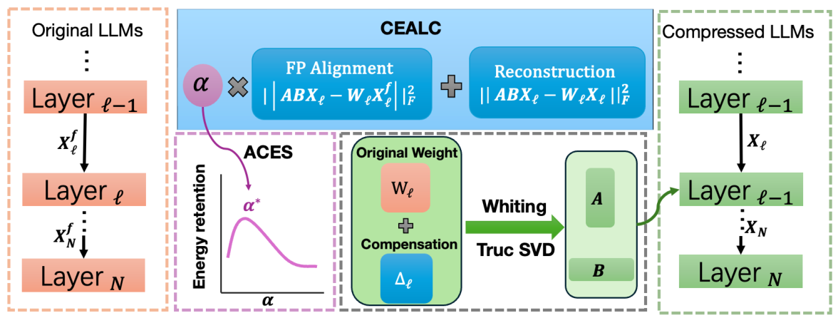
Figure 2 (paper Fig. 2): original and compressed activation paths feed a compensation-aware factorization. Cropped from Hu et al., CC BY 4.0. The diagram combines reference alignment, spectral coefficient selection and factor construction; these are separate computational stages.

4. The exact low-rank solution, including what it cannot fit

Assume first that $H=XX^\top$ is positive definite. Define the orthogonal projector onto the row space of $X$,

$$P=X^\top H^{-1}X,\qquad \|UX-Z\|_F^2=\|UX-ZP\|_F^2+\|Z(I-P)\|_F^2. \tag{5}$$

To justify this decomposition, note that $XP=X$, so every possible $UX$ already lies in that row space. Its difference from $ZP$ is orthogonal to $Z(I-P)$. The cross term vanishes in the squared Frobenius norm. The second term is an irreducible component for this layer and this calibration matrix, even before imposing a rank budget.

This is a useful corrective to the language of error compensation. If two original states have become indistinguishable on the compressed path, one fixed linear map of the compressed states cannot reconstruct both original outputs. The theorem optimizes over attainable outputs; it does not reconstruct information by assumption.

Let $M=ZX^\top$. Expanding the remaining objective using traces yields a quadratic term $\operatorname{tr}(UHU^\top)$ and a cross term $-2\operatorname{tr}(UM^\top)$. Since the symmetric square root $H^{1/2}$ is invertible, completing this square produces an equivalent rank-constrained problem in $V=UH^{1/2}$:

$$\min_{\operatorname{rank}(U)\leq r}\|UX-Z\|_F^2 \quad\Longleftrightarrow\quad \min_{\operatorname{rank}(V)\leq r}\|V-MH^{-1/2}\|_F^2. \tag{6}$$

The double arrow denotes corresponding minimizers, not equality of objective values. Rank is preserved under multiplication by an invertible matrix. This is why applying the Eckart-Young-Mirsky theorem is legitimate after the change of coordinates.

Now define $\Delta=(X^f-X)X^\top$. Substituting Equation (4), the target’s cross moment is $M=W(H+\beta\Delta)$. No $N\times N$ projector needs to be explicitly formed. The full solution is

$$\begin{aligned} G(\beta)&=W(H+\beta\Delta)H^{-1/2},\\ [G(\beta)]_r&=\widetilde U_r\Sigma_r\widetilde V_r^\top,\\ A&=\widetilde U_r\Sigma_r^{1/2},\qquad B=\Sigma_r^{1/2}\widetilde V_r^\top H^{-1/2}. \end{aligned}\tag{7}$$

Multiplying the factors gives $U=[G]_rH^{-1/2}$. Truncation occurs in the activation-weighted coordinates, and the final right factor maps back to the original input coordinates. Splitting the singular values equally between the factors is a convenient parameterization; assigning all of them to one factor gives the same product in exact arithmetic, though finite-precision and later quantization behavior can differ.

5. Statistics, regularization and the cost of calibration

The compact statistics are both $n\times n$, independent of the number of calibration tokens. For $n=4096$, $N=128\times2048$ and FP32 storage, two complete activation matrices would occupy 8 GiB, while two second-moment matrices occupy 128 MiB. This calculation excludes the model, forward-pass workspaces, decompositions and temporary activations. It illustrates the memory trade-off without claiming the paper’s broad storage comparison holds for every model or layer.

The residual cross moment $\Delta$ is generally not symmetric. Replacing it by a symmetric covariance would lose information about how original-path deviations correlate with the current input. Both streams must have the same normalization and token masking. Padding tokens, unmatched batches or statistics collected before upstream factors are installed can change the mathematical target while leaving matrix dimensions apparently correct.

Algorithm 1. Collect paired statistics for a fixed upstream model

This is a mathematical streaming version of Appendix A.11. It uses raw sums so the normalization is explicit.

1. Fix the already-compressed upstream layers and calibration examples.
2. Set H = 0, Delta = 0, token_count = 0.
3. For each calibration batch, obtain matching X and X_ref.
4. Flatten valid token positions to columns; keep their order identical.
5. Accumulate H += X X^T.
6. Accumulate Delta += (X_ref - X) X^T.
7. Increase token_count by the number of valid columns.
8. Optionally divide both matrices by the same token_count.
9. Return H, Delta and the normalization convention.

The paper’s streaming listing rescales previous statistics by $t/(t+m)$ and adds new outer products scaled by $2/(t+m)$. Under a consistent token counter, induction shows that the result is twice the running mean of the raw outer products. This is equivalent to common scaling of $H$ and $\Delta$ for the undamped mathematical solution. It is not an exponential moving average with a fixed forgetting factor, despite that terminology appearing in the complexity section.

With no ridge, multiplying both statistics by $c>0$ multiplies $G$ by $\sqrt c$ and the inverse square root by $1/\sqrt c$, leaving the reconstructed $U$ unchanged. With a ridge, the ridge must also scale by $c$ to preserve this invariance. Reporting only the scalar value of a damping parameter without its normalization convention is therefore incomplete.

Full row rank is an assumption, not a consequence of having more tokens than channels. Correlated channels can still make $H$ singular. Appendix A adds $\lambda I$. Algebraically, retaining $M=ZX^\top$ and replacing the metric by $H+\lambda I$ corresponds to a regularized problem:

$$\min_{\operatorname{rank}(U)\leq r} \|UX-Z\|_F^2+\lambda\|U\|_F^2 \quad\Longrightarrow\quad U=[M(H+\lambda I)^{-1/2}]_r(H+\lambda I)^{-1/2}. \tag{8}$$

This follows by adding $\lambda\operatorname{tr}(UU^\top)$ to the quadratic expansion. It is not exactly the undamped theorem. The distinction matters in low-variance directions, where regularization deliberately biases the fitted map. In addition, a Cholesky factor is not the symmetric matrix square root. A derivation using $H=CC^\top$ can use $UC$ and $MC^{-\top}$ consistently; mixing symmetric-root and triangular-root orientations would define a different transformation.

6. ACES chooses a target that is easier to truncate

For coefficient selection, define $S=WHH^{-1/2}$ and $D=W\Delta H^{-1/2}$, or their consistently damped versions. Then $G(\beta)=S+\beta D$. The exact retained energy ratio is

$$\operatorname{RER}(\beta)= \frac{\sum_{i\leq r}\sigma_i(G(\beta))^2}{\|G(\beta)\|_F^2} =1-\frac{\sum_{i>r}\sigma_i(G(\beta))^2}{\|G(\beta)\|_F^2}. \tag{9}$$

The ratio asks how concentrated this target is in its leading singular directions. It is scale-invariant, and changing $\beta$ changes the target itself. A higher ratio is not a guarantee of lower absolute reconstruction error, lower downstream loss, or better calibration generalization. It is a principled structural heuristic whose connection to task quality must be tested.

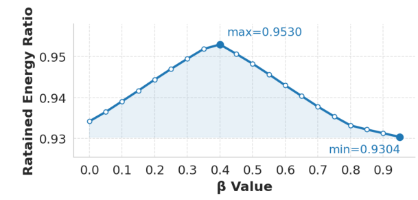
Figure 3 (paper Fig. 1c): retained energy depends non-monotonically on the compensation coefficient. Cropped from Hu et al., CC BY 4.0. The curve supports coefficient adaptation for this example, without establishing a universal coefficient schedule.

Repeatedly computing an SVD for many candidate coefficients would be expensive. ACES computes the leading left and right subspaces of $S$ once, with bases $U_r,V_r$, and fixes their orthogonal-complement projectors $P_L=I-U_rU_r^\top$ and $P_R=I-V_rV_r^\top$. It approximates the changing tail by $S_\perp+\beta D_\perp$, where the two matrices are doubly projected.

For clarity I use $q$ for the squared tail ratio. The paper alternates between squared and unsquared ratios; they have the same minimizer wherever the denominator is positive. Expanding the numerator and denominator gives

$$\widetilde q(\beta)=\frac{a+2b\beta+c\beta^2}{A_0+2B_0\beta+C_0\beta^2}, \tag{10}$$

where $a=\|S_\perp\|_F^2$, $b=\langle S_\perp,D_\perp\rangle_F$, $c=\|D_\perp\|_F^2$, and $A_0,B_0,C_0$ are the corresponding quantities for $S,D$. These capital coefficients are scalars, unrelated to the low-rank factors $A,B$.

Let numerator and denominator be $n(\beta),d(\beta)$. The quotient rule gives $\widetilde q'=(n'd-nd')/d^2$. The cubic terms cancel, leaving

$$\frac{n'd-nd'}{2} =(cB_0-bC_0)\beta^2+(cA_0-aC_0)\beta+(bA_0-aB_0). \tag{11}$$

Thus a continuous constrained search becomes evaluation of real stationary roots and interval endpoints. This is exact minimization of the rational surrogate, subject to handling a zero denominator and degenerate polynomial. It is still only approximate minimization of the true spectral tail ratio.

7. Why the frozen subspace can become inaccurate

Appendix A.3 invokes a positive gap $\delta=\sigma_r(S)-\sigma_{r+1}(S)$ and a small perturbation relative to that gap:

$$\tau=\frac{\beta\|D\|_2}{\delta}\ll1. \tag{12}$$

A small gap means the boundary between retained and discarded subspaces is unstable. Even a modest compensation term can rotate that boundary. An approximation derived near $\beta=0$ should not automatically be trusted throughout $[0,1]$. Clipping or shrinking the coefficient can reduce the perturbation, but the paper’s qualitative example of $\tau\lesssim0.5$ is not a universal accuracy threshold established by a reported constant.

The doubly projected matrix is also not generally the residual of a feasible fixed rank-$r$ reconstruction. Off-diagonal blocks connecting retained and discarded subspaces can rotate singular vectors. Discarding their effect makes sense as a local surrogate, but it does not turn the score into an upper bound on actual truncation loss.

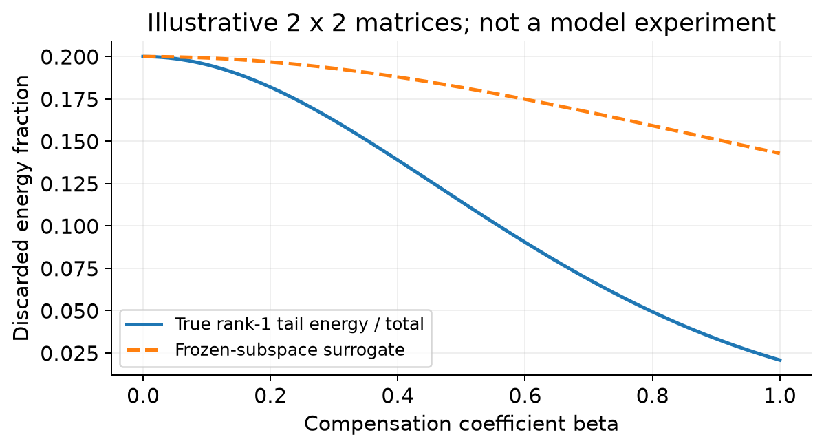
Figure 4 (original explanatory calculation): exact and surrogate squared tail ratios for the two-by-two matrices specified below, at rank one. This is an analytical illustration, not a model experiment. Agreement near zero does not imply agreement for a large perturbation.

Take S to be diagonal with entries 2 and 1, and D to have zeros on the diagonal and ones off the diagonal. The fixed bottom-right block is always 1. The true smaller eigenvalue is $(3-\sqrt{1+4\beta^2})/2$, while total squared energy is $5+2\beta^2$. The plotted curves follow directly from these expressions. At $\beta=1$, the true squared tail ratio is about 0.0208 and the surrogate is about 0.1429. This is not a counterexample to the local theorem: here $\tau=1$, outside its small-perturbation regime.

There is a further mathematical qualification. Turning a second-order bound on tail energy into a second-order bound on the unsquared tail ratio requires care near zero tail energy. A square root is not uniformly Lipschitz at zero, and division also requires total energy bounded away from zero. I would therefore rely most directly on the squared-energy surrogate and treat the appendix’s ratio bound as needing explicit non-degeneracy qualifications.

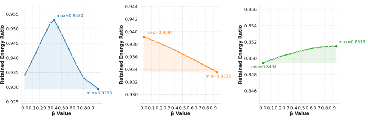
Figure 5 (paper Fig. 5): different layers can prefer different compensation coefficients. Cropped from Hu et al., CC BY 4.0. Its caption says rank 1228 whereas Fig. 1c says rank 128; these should not be combined into one calibrated experiment without clarification.

8. Three procedures, with explicit numerical boundaries

Algorithm 2. Select beta from a fixed-subspace surrogate

This is a clarified mathematical procedure based on ACES. The safeguards make special cases explicit; they are not a claim about a particular software implementation.

1. Form a consistent whitener L; compute S = W H L and D = W Delta L.
2. Compute the leading rank-r singular subspaces of S.
3. Project S and D onto both complementary subspaces.
4. Compute a, b, c, A0, B0, C0 in Equation (10).
5. Form the quadratic stationary polynomial in Equation (11).
6. If quadratic, find real roots; if linear, solve the linear equation.
7. If constant or identically zero, retain the interval endpoints.
8. Add all valid roots and endpoints to the candidate set.
9. Apply the declared cap/shrink convention and final feasible bounds.
10. Reject candidates whose total-energy denominator is numerically zero.
11. Evaluate the squared ratio; choose its smallest valid value.
12. Return beta; map to alpha only when beta < 1.

Appendix Algorithm 3 prints a ratio branch followed by an energy-only candidate assignment without a clear separating else. Its surrounding explanation distinguishes two objectives. I interpret those as alternatives rather than letting the second assignment erase the first candidate set. For the energy objective, minimizing $a+2b\beta+c\beta^2$ gives the clipped value $-b/c$ when $c>0$. It optimizes absolute surrogate tail energy, a different criterion from the ratio.

The order of guardrails also matters. Shrinking a clipped coefficient by a factor below one can move it below the declared lower bound. A clear procedure must state whether the final feasible interval applies before or after shrinking. No paper theorem resolves an ambiguous operational convention automatically.

Algorithm 3. Compress a network sequentially

The reference path remains original while the compressed path changes after each replacement. This ordering is what gives the cross-residual statistic its intended meaning.

1. Choose layer ranks, calibration data, ridge scaling and beta bounds.
2. Keep a fixed reference model and a current compressed model.
3. For the next layer, collect paired statistics with Algorithm 1.
4. Use a supplied beta or select it with Algorithm 2.
5. Form G = W (H + beta Delta) L.
6. Compute a rank-r truncated SVD of G.
7. Construct A and B using the consistent whitening convention.
8. Replace this layer in the compressed path with the two factors.
9. Recompute downstream calibration inputs after the replacement.
10. Continue in dependency order; evaluate the final compressed model.

CEALC with a supplied coefficient needs one factorization of $G$. Adaptive ACES additionally extracts a subspace from $S$. The full adaptive procedure therefore normally involves two truncated decompositions per layer. Appendix A.10 states the extra SVD explicitly. The main-text description of a single SVD per layer is accurate only for the final fixed-coefficient factorization, not as a complete count for the adaptive pipeline.

The statistics can be collected without retaining all calibration activations, but streaming does not make collection free. Each layer requires matrix products scaling with token count and width; its second-moment storage is quadratic in width. A truncated solver may have cost roughly proportional to $mnr$, depending on algorithm and iterations. Such an estimate is not the cost of an arbitrary dense exact SVD. Compression-time comparisons should state which routine and accuracy tolerance are assumed.

9. Main results: read the table before the headline

Table 1 reports LLaMA-7B results at compression ratios 0.2, 0.4 and 0.6. I preserve the paper’s reported ratio rather than inferring an exact whole-model byte budget. The table’s uncompressed baseline is WikiText-2 perplexity 5.68 and reported average zero-shot accuracy 0.52.

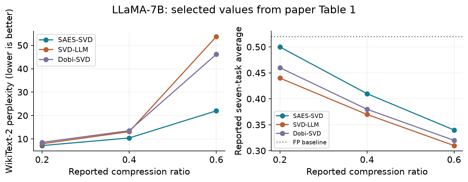
Figure 6 (redrawn from paper Table 1): selected perplexity and reported average-accuracy values for LLaMA-7B. These are authors’ measurements, not new experiments. The three methods’ training and rank-allocation budgets differ in the reported comparison.

At ratio 0.2, SAES-SVD reports WikiText-2 perplexity 7.17 and average accuracy 0.50, compared with Dip-SVD’s 7.95 and 0.47. Using rounded accuracy values, the drop from the baseline decreases from 0.05 to 0.02, a 60% reduction in the drop. Using the printed relative-drop column, $1-3.9/9.2$ gives 57.6%, consistent with the approximately 58% statement. Rounding explains this small difference.

The analogous perplexity-gap calculation is different:

$$1-\frac{7.17-5.68}{7.95-5.68}\approx0.344. \tag{13}$$

That is a 34.4% reduction in the WikiText-2 gap, not the introduction’s 52% relative to Dip-SVD. A different aggregation might produce another number, but the paper does not identify it clearly enough here to reconstruct that headline. I would report the table values and the precise denominator instead.

At ratio 0.6, WikiText-2 perplexity improves from Dobi-SVD’s 46.18 to 22.01, and the gap above the baseline shrinks by about 59.7%. This is a substantial relative improvement. Nevertheless, average accuracy is 0.34 versus the baseline’s 0.52, an absolute drop of 0.18. The main text’s claim of a drop below 0.03 at this ratio is inconsistent with Table 1. Better than a degraded baseline is not the same as preserving near-original quality.

The result is not uniform across corpora. At ratio 0.4, SAES-SVD reports C4 perplexity 32.79 versus Dobi-SVD’s 23.54, so Dobi-SVD is better on that entry. At ratio 0.2, Dobi-SVD also has lower PTB and C4 perplexity. I read SAES-SVD as strong on several reported aggregate and WikiText-2 comparisons, not as winning every task and dataset.

There are additional table-quality issues. Table 1’s caption says Dip-SVD’s ratio-0.4 result was unavailable, yet a row is present. Its FWSVD ratio-0.2 per-task values average to about 0.077, while the printed average is 0.02. Table 5’s original row lists four accuracies whose arithmetic mean is about 74.74%, rather than the printed 68.85%. These problems do not erase the method, but they prevent treating every aggregate as independently reconciled evidence.

10. Ablations, extensions and what the runtime measures

The component ablation in Table 3 gives a cleaner local comparison. LLaMA-2-7B WikiText-2 perplexity changes from 9.34 without either component to 7.66 with CEALC and 7.37 with both components. For LLaMA-3-8B it changes from 16.59 to 12.25 to 11.48. The corresponding four-task accuracies are 58.66%, 62.02%, 63.03% and 55.76%, 58.82%, 60.18%. These are four-task averages and should not be merged with Table 1’s seven-task average.

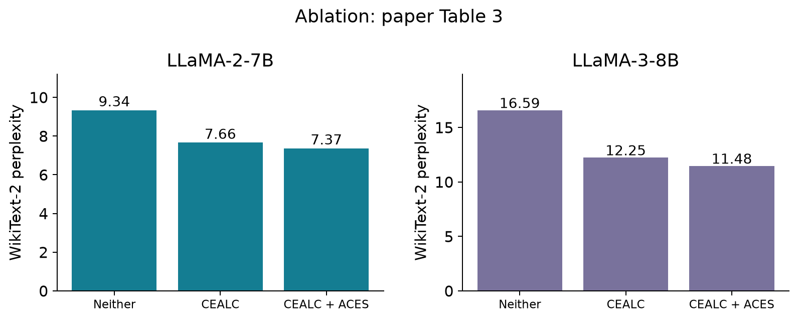
Figure 7 (redrawn from paper Table 3): CEALC accounts for the larger first improvement in these two ablations; ACES provides a further gain. This figure shows perplexity only and does not combine differently defined accuracy averages.

Table 4 shows sensitivity to the allowed coefficient interval: the printed $[0,1]$ setting gives PPL 8.96, while $[0.25,0.75]$ gives 7.37. This is evidence that unrestricted adaptation is not automatically best. However, the table labels its bounds $\alpha$ while ACES optimizes $\beta$. Those intervals are not interchangeable. If the bounds refer to $\alpha$, $[0.25,0.75]$ maps to $\beta\in[0.2,0.4286]$; if they refer to $\beta$, the corresponding $\alpha$ interval is $[1/3,3]$. I leave the experimental convention unresolved.

Appendix Table 7 broadens the evidence to LLaMA3.1 and Qwen2.5, with long-context, coding and mathematical tasks at ratio 0.2. For example, Qwen2.5-7B HumanEval is 0.66 for the original model, 0.55 for SVD-LLM and 0.63 for SAES-SVD. This is encouraging coverage, but a single compression level and limited evaluation details do not establish robustness at larger reductions, under domain shift, or on long agent trajectories.

Table 8 adds mixed-rank allocation and improves ratio-0.4 WikiText-2 PPL from 10.42 to 7.48 and average accuracy from 0.41 to 0.47. That supports complementarity between coefficient selection and rank allocation. They solve different problems: one chooses the target at a fixed rank; the other reallocates capacity across matrices.

Table 10 combines SAES with GPTQ at an equivalent three-bit budget. LLaMA2-7B PPL changes from 10.17 to 7.64 and Qwen2.5-7B from 12.29 to 9.87. Effective bits must include the factor shapes and quantization metadata before equal memory can be assumed in a deployment. The result motivates a combination study; it does not guarantee equal latency to direct three-bit quantization.

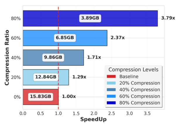
Figure 8 (paper Fig. 4): LLaMA-3-8B memory usage and speedup on an NVIDIA A6000. Cropped from Hu et al., CC BY 4.0. The reported 1.29x to 3.79x range belongs to these configurations; the figure alone does not specify a universal serving speedup.

Two smaller matrix products reduce arithmetic and weight traffic but introduce an intermediate activation and another operation boundary. Batch size, sequence length, prefill versus decoding, precision and kernel efficiency determine the net benefit. The paper’s speed figure omits enough workload detail that I would not use its maximum value as a capacity-planning multiplier. Accuracy at that compression level also belongs in the same decision.

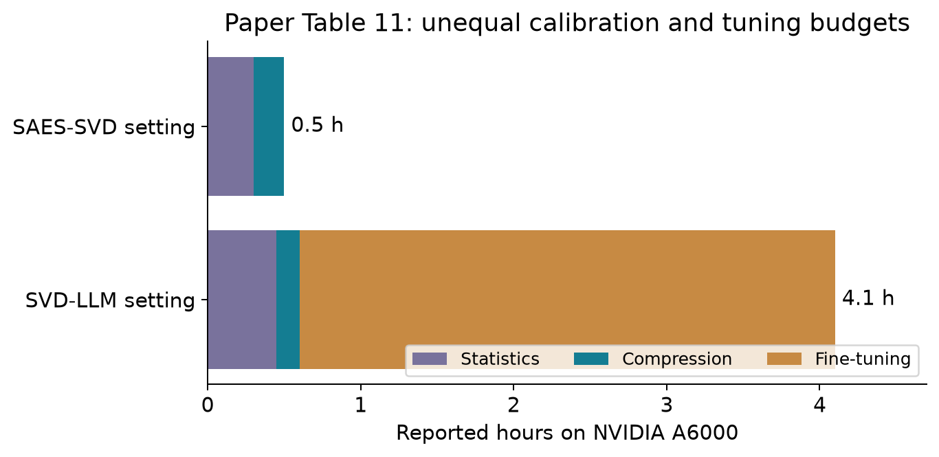
Figure 9 (redrawn from paper Table 11): the 4.1-hour versus 0.5-hour comparison includes fine-tuning only in the SVD-LLM configuration and uses 256 versus 128 calibration samples. It measures the reported pipelines, not an isolated factorization speed difference.

The reduction is $1-0.5/4.1\approx87.8\%$. In the compression-only column, SAES-SVD is actually 0.20 hours versus 0.15 hours. The practical saving comes mostly from omitting the 3.5-hour fine-tuning phase. This is useful evidence for a training-free workflow, but not proof that SVD-LLM intrinsically requires that fine-tuning configuration or that ACES is computationally cheaper.

11. Limitations: where the correction stops helping

The strongest exact guarantee is conditional on a fixed calibration matrix, fixed target coefficient and a specified metric. It does not establish optimality of the sequence of compressed layers. Replacing a layer changes the inputs of later layers and the distribution on which their objectives are constructed. A greedy sequence of optimal local fits can remain globally suboptimal.

Reference alignment can also overfit the calibration pairs. If the relation between $X^f-X$ and $X$ changes in another domain, $\Delta$ may encode an unhelpful correction. The original model is a reference for preservation, not an oracle for correctness. Recovering its internal activations need not improve an instruction-following or safety metric that is absent from the evaluation.

The uncentered second moments emphasize energetic directions and frequent tokens. Rare but consequential contexts can have low weight in this metric. A small Frobenius residual can coexist with a changed answer on a difficult example. Fisher weighting, task-aware validation or subgroup-aware calibration are possible alternatives, each introducing estimation cost and its own assumptions.

Width creates a separate boundary. Two $n\times n$ statistics, matrix square roots and subspace extraction can be expensive for wide feed-forward inputs. A smaller calibration set reduces collection time, but may worsen conditioning or coverage. Streaming avoids storing every token activation; it does not remove the quadratic dependence on channel count.

Finally, evidence quality is a practical limitation of v1. Several captions, averages and coefficient labels need clarification. Appendix Fig. 6’s caption names LLaMA2-7B while nearby prose names LLaMA3-8B. I would not infer a universal depth-dependent beta schedule from that plot. These inconsistencies are reasons to constrain claims and request precise experimental definitions, rather than to substitute guessed corrections.

12. Independent critical analysis: what I would test next

My main concern is that ACES optimizes the compressibility of a moving target. A ratio can improve because the denominator grows, because the tail shrinks, or because the reference mixture becomes easier to fit. Those possibilities have different implications for model quality. A useful follow-up would record true retained-energy ratio, absolute output error against both targets, and held-out token loss for the same coefficient sweep. Their correlations would reveal when spectral concentration is a useful proxy and when it becomes misleading.

A second concern is the unmeasured trust region for the frozen subspace. The paper states a gap-and-perturbation condition, but the reported experiments do not map observed $\tau$ to approximation error across all compressed layers. I would stratify layers by spectral gap, compare the analytical coefficient against a small exact-SVD grid, and report both extra compression time and task benefit. A conditional refinement only for unstable layers would make the trade-off visible. This is an evaluation proposal, not an experiment performed here.

Third, the sequential procedure should separate recoverable drift from destroyed information. Equation (5) identifies an irreducible component $Z(I-P)$, while Equation (7) identifies additional rank-truncation error. Reporting their relative sizes would help diagnose why some layers resist compensation. If irreducible error dominates, increasing the local rank may not recover what the upstream representation lost; preserving more upstream capacity could be more effective.

Fourth, the strongest end-to-end time claim deserves matched budgets. I would compare the same calibration examples, equal factor parameter counts, the same precision and both training-free and fine-tuned variants where meaningful. That comparison would distinguish improvements due to the target, rank allocation, calibration count and training budget. It would also allow the table averages and baseline protocols to be recomputed consistently.

Fifth, the deployment test should expose the full quality-cost frontier. For each supported model, report resident weight bytes including metadata, peak working memory, prefill latency, decode latency at several batch sizes, and representative task quality. A nominal compression ratio or maximum speedup is too incomplete for choosing a production configuration. Low-rank compression becomes compelling when it moves this frontier under the workload the user actually serves.

A compact evidence checklist for such a study is: identify the model and calibration distribution; distinguish alpha from beta; specify moment normalization and damping; state the rank-to-budget conversion; report the exact task sets behind averages; expose uncertainty across calibration seeds; and compare quality at matched memory and workload. None of this requires treating a paper’s qualitative conclusion as a substitute for measurement.

13. Conclusion

SAES-SVD gives a clean answer to a specific compression problem: a later layer should be allowed to compensate for predictable drift created by earlier layers. CEALC expresses that idea as a blended output target, then reduces rank-constrained regression to a whitened SVD. ACES supplies an inexpensive coefficient heuristic by optimizing a rational approximation to discarded spectral energy.

I regard the exact regression derivation as the most reusable contribution. It exposes what is fitted, what information is unavailable to the local map, and how second-order statistics replace large activation matrices. The adaptive coefficient is useful but more conditional: its approximation depends on subspace stability and its objective is a proxy for task quality. The experiments support further investigation, while the numerical inconsistencies and unmatched budgets make restrained reporting essential.

The practical lesson is to preserve the distinction between local mathematical optimality, empirical language-model quality and measured serving efficiency. SAES-SVD connects these levels more thoughtfully than a raw weight-space truncation, but it does not collapse them into one guarantee.

References and figure attribution

1. Xing Hu, Dawei Yang, Yuan Cheng, Zhixuan Chen and Zukang Xu. SAES-SVD, arXiv v1, 2026. Primary source for Sections 3-10 and all reported model results; the complete PDF and Appendix A were read.
2. Carl Eckart and Gale Young. The approximation of one matrix by another of lower rank, 1936. The low-rank approximation theorem used by the primary paper.
3. Figures 1, 2, 3, 5 and 8 reproduce cropped portions of the primary paper under its CC BY 4.0 license. Figures 6, 7 and 9 redraw stated table values; Figure 4 is an explicitly specified analytical example. Figure numbers in this review are independent of the source paper’s numbering.