TTT-E2E: Learning a Long Context into Weights

Review date: October 7, 2026
Author: Zhongzhu Zhou
Paper reviewed: End-to-End Test-Time Training for Long Context
Paper authors: Arnuv Tandon, Karan Dalal, Xinhao Li, Daniel Koceja, Marcel Rød, Sam Buchanan, Xiaolong Wang, Jure Leskovec, Sanmi Koyejo, Tatsunori Hashimoto, Carlos Guestrin, Jed McCaleb, Yejin Choi, Yu Sun
arXiv and version: 2512.23675v2, December 31, 2025

1. The useful question is what a memory must preserve

I read TTT-E2E as a proposal to change the object that carries a language model’s history. Full attention retains a growing collection of keys and values. A recurrent model compresses history into a state of fixed size. This paper makes a subset of the model’s weights that state, and uses ordinary next-token learning to update it. Recent tokens remain available through sliding-window attention; older experience can influence predictions through the adapted weights.

The proposal is not simply to fine-tune a deployed model whenever new text arrives. The initialization is trained in advance for the sequence of updates it will undergo. Each training sequence becomes a miniature learning problem. The outer training process rewards an initialization whose future predictions improve after the inner updates. This alignment between how the model is trained and how it will change at inference is the second half of the method.

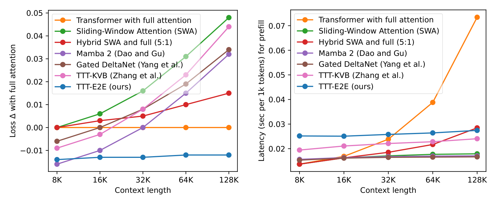
Figure 1 (paper Fig. 1). The left panel reports loss relative to full attention; lower is better. The right panel measures seconds per 1K prefill tokens on one H100, with 128K total tokens per batch. Its nearly flat curve means approximately constant work per token, not constant total time to read an arbitrarily long document.

The main experiment uses models described as 3B, trained with a reported 164B tokens, and context lengths up to 128K. TTT-E2E shows strong average language-modeling performance across these lengths and reports a 2.7-fold prefill speed advantage over full attention at 128K. Those results are interesting precisely because another result is unfavorable: exact needle retrieval remains much weaker than full attention. Both findings belong in the central explanation.

My interpretation is that this is a promising method for predictive compression. It learns features of a stream that help predict what comes next. It does not establish a general replacement for a searchable record of every fact. Repeated narrative patterns and an arbitrary identifier hidden in a document place different demands on memory. A system designer needs to know which demand the application imposes before deciding that a smaller or faster memory is better.

This review follows all 29 pages of v2, including Appendices A-D. The source figures retain the authors’ measurements. Additional equations below are explanatory derivations, and the scalar stability example is a mathematical illustration rather than an experiment with their model. I distinguish a result at a measured scale from an expectation about future production models.

2. Prerequisites: attention, recurrence, and predictive loss

2.1 Why full attention gets expensive

Let the context contain $T$ tokens, with a fixed model width and layer count. During causal prefill, token $t$ can attend to approximately $t$ positions. Summing these interactions gives:

$$N_{\mathrm{full}}(T)=\sum_{t=1}^{T}t =\frac{T(T+1)}{2},\qquad N_{\mathrm{window}}(T)\leq Tk. \tag{1}$$

Here $k$ is a fixed sliding-window length. Equation (1) counts attention interactions, not the complete floating-point workload. Projection and MLP costs remain, as do memory movement and kernel overhead. Nevertheless, it explains why full-attention prefill grows quadratically in context length while a fixed window grows linearly. During decoding, full attention scans an expanding cache for each new token, whereas a fixed window limits that scan.

Reducing this cost discards direct access to distant keys and values. A recurrent state provides another route for history to affect the output. Formally, a recurrence has a state transition and an output rule:

$$s_t=F(s_{t-1},x_t),\qquad \widehat p_{t+1}=G(s_t,x_t). \tag{2}$$

TTT interprets the fast weights as part of $s_t$. The transition $F$ contains a gradient update. This does not make the system free of recurrence: successive updates still depend on their predecessors. It changes the form and capacity of the recurrent state. The full deployed state also includes a bounded local attention cache and any working state required by the update procedure.

2.2 Compression is judged by a task

For the next observed token $x_t$, cross entropy is $-\log \widehat p_t(x_t)$. The loss asks whether the model assigned probability to the actual next symbol. It does not directly ask whether a string observed ten thousand tokens earlier can be reproduced exactly. A compressed representation can be excellent for the first objective and poor for the second without a logical contradiction.

Average loss and perplexity also need careful interpretation. If $L$ is average natural-log cross entropy, perplexity is $\exp(L)$. A loss difference $\Delta L$ changes perplexity by a multiplicative factor $\exp(\Delta L)$. Thus a loss improvement of 0.018, reported in one of the paper’s 8K ablations, corresponds to about a 1.8% reduction in perplexity. It is not an improvement of 1.8 percentage points in question-answering accuracy.

There are three timescales to keep separate. The outer optimization operates over many training sequences. Within a sequence, the inner update changes fast weights every chunk. Within a chunk, causal attention handles immediate context. Calling all three processes training obscures which information can influence each prediction. The central correctness condition is temporal: a token must be predicted before its own label is used to update the weights that predicted it.

I will use $W$ for fast weights and $\phi$ for weights held fixed during the inner loop. Both may be learned by the outer process. Inner-loop freezing therefore does not imply that the corresponding layer was never trained. This distinction matters for the embeddings, attention layers, normalization layers, and static MLP branches in the final architecture.

3. From a memoryless predictor to causal adaptation

The paper starts with a deliberately weak toy model: remove attention from a Transformer and let a feed-forward network predict the next token from the previous token. With fixed weights, this model cannot consult the preceding document. Giving it trainable state changes the situation. Past observations influence the weights used for later predictions, even though they are no longer supplied as an attention sequence.

Let $f(x;W)$ produce a distribution over the vocabulary. For clarity, temporarily omit the static parameters. Define the token loss and the inner update as

$$\ell_t(W)=-\log f(x_{t-1};W)[x_t],\qquad W_t=W_{t-1}-\eta\nabla_W\ell_t(W_{t-1}). \tag{3}$$

The order is essential. First predict $x_t$ with $W_{t-1}$; next reveal $x_t$; then update to $W_t$. The update may improve the prediction of $x_{t+1}$, but it cannot retroactively improve the recorded prediction of $x_t$. This is ordinary causal online learning, embedded inside a language model. Test-time training here does not require labels from a human: the next token in the observed context provides the learning signal.

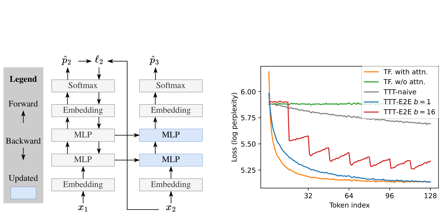
Figure 2. Paper Figure 2, cropped from PDF page 3. The toy model makes the distinction between an outer objective that anticipates adaptation and one that ignores it visible. The simplified network is an explanatory starting point, not the final competitive model.

A naive approach first trains a static predictor and only turns on updates at inference. That asks the same initialization to serve two different purposes without explicitly training it for the second. TTT-E2E instead optimizes the losses encountered along the adaptation trajectory:

$$\mathcal L_{\mathrm{adapt}}(W_0;X) =\frac{1}{T}\sum_{t=1}^{T}\ell_t(W_{t-1}), \qquad \mathcal L_{\mathrm{static}}(W_0;X) =\frac{1}{T}\sum_{t=1}^{T}\ell_t(W_0). \tag{4}$$

These objectives share the same labels but not the same computation graph. In the first objective, changing $W_0$ changes every later update and every later prediction. A good initialization is therefore one from which a short sequence of local gradient steps makes useful progress. The outer process can learn features and loss geometry that make the inner learning rule effective.

An analogy is useful if kept narrow. A student can be trained to answer a fixed exam, or trained to learn from a small set of examples before answering a new exam. TTT-E2E pursues the second kind of competence for token prediction. The analogy does not imply human-like understanding, an explicit database, or guaranteed retention of facts. The information is represented in parameter changes optimized for future predictive loss.

The toy example also explains why merely enabling gradients is insufficient. A large update can erase useful behavior. A small update can do essentially nothing. An update that reduces the loss on the just-observed token can still hurt later tokens. The outer objective judges updates by their downstream consequences across training sequences, although it cannot guarantee good consequences for every future document.

4. Deriving the meta-gradient

4.1 One update already requires a second derivative

Consider an inner chunk loss $A(W)$, one update $U(W)$, and a later loss $B(U)$. Hold the inner step size and static parameters fixed for this derivation:

$$U(W)=W-\eta\nabla A(W),\qquad \frac{\partial U}{\partial W}=I-\eta H_A(W), \tag{5}$$

where $H_A$ is the Hessian of $A$. Applying the chain rule gives

$$\nabla_W B(U(W)) =\left(I-\eta H_A(W)\right)^\top\nabla_U B(U(W)). \tag{6}$$

There are two effects. Moving $W$ directly changes the starting predictor, represented by $I$. It also changes the gradient that the inner optimizer will take, represented by $-\eta H_A$. Dropping the latter term changes the training objective’s gradient. End-to-end differentiation includes this dependence; it is not just ordinary training on a concatenation of chunks.

No dense Hessian needs to be stored. Equation (6) requires the action of a Hessian on a vector, which automatic differentiation can compute without forming every pairwise second derivative. Nevertheless, supporting these derivative operations through attention and retaining or recomputing the required intermediate values has a substantial systems cost.

4.2 Many updates expose a conditioning problem

For chunk losses $A_i$ and fast-weight states $W_i$, define $J_i=\partial W_i/\partial W_0$. Then

$$\begin{aligned} J_0&=I,\\ J_i&=\left(I-\eta H_{A_i}(W_{i-1})\right)J_{i-1},\\ \nabla_{W_0}\mathcal L &=\frac{1}{N}\sum_{i=1}^{N}J_{i-1}^{\top}\nabla A_i(W_{i-1}). \end{aligned} \tag{7}$$

This equal-size-chunk expression suppresses the additional paths through static parameters and assumes a fixed step size. It is a derivation of the central dependency, not a complete specification of every training hyperparameter. The products of Jacobians make the relation to training recurrent networks explicit: information about a distant loss can shrink or grow as it travels back through many transitions.

Take a one-dimensional illustrative loss $A(w)=a(w-w_\star)^2/2$. Gradient descent gives

$$e_i=w_i-w_\star=(1-\eta a)e_{i-1},\qquad |e_i|<|e_{i-1}|\ \Longleftrightarrow\ 0<\eta a<2. \tag{8}$$

For nonzero error and $a>0$, require $|1-\eta a|<1$. It is a local quadratic example, not a stability theorem for the paper’s nonconvex network. Still, it explains why more inner steps are not automatically better and why changing the chunk size can change both hardware efficiency and optimization behavior.

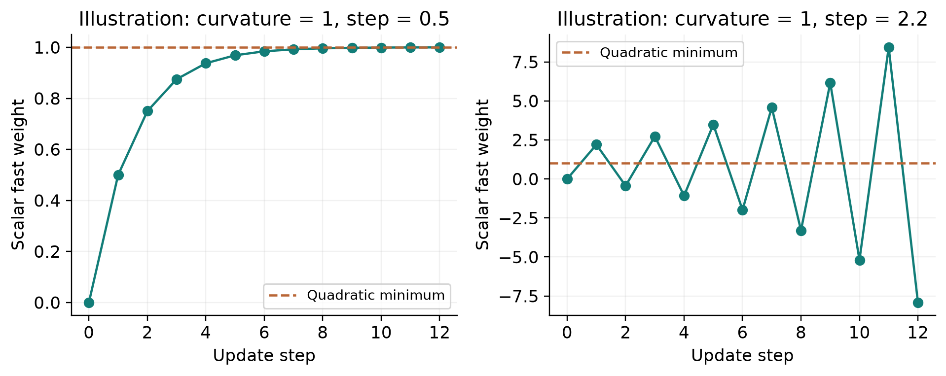
Figure 3. Original explanatory plot for $a=1$, $w_\star=1$, and $w_0=0$. The two step sizes are chosen to illustrate Equation (8); these are not TTT-E2E measurements or recommended model hyperparameters.

An outer learner might shape the initialization so that the updates encountered in training become useful and well conditioned. It does not eliminate sensitivity to distribution shifts, document length, or unusually large gradients. The later ablations should be read in this light: architectural restrictions are also restrictions on a difficult differentiable dynamical system.

5. Why batching needs a sliding window

Updating after every token creates a highly sequential computation. The paper batches the inner updates. If chunk $i$ contains $b$ token targets, its average loss and update are

$$A_i(W)=\frac{1}{b}\sum_{t=(i-1)b+1}^{ib}\ell_t(W),\qquad W_i=W_{i-1}-\eta\nabla A_i(W_{i-1}). \tag{9}$$

Every target in that chunk is scored using the same pre-update weights. The update is applied only after the chunk has been scored. Batching amortizes optimizer work and enables parallel computation, but the fast weights cannot yet contain information learned from earlier targets in the same chunk. The toy model’s sawtooth loss pattern illustrates this staleness.

The final model combines the adaptive state with causal sliding-window attention. Local attention supplies the recent tokens that the frozen-within-chunk weights have not yet absorbed. The adopted configuration uses an 8K attention window and 1K inner chunks. With a window at least as large as the chunk, the model can directly access earlier positions within the chunk without waiting for the next parameter update.

This division of labor is the core architectural argument. Attention handles detailed short-range context. Fast weights summarize information across chunks. Neither component has to solve the other’s problem perfectly. A causal mask remains necessary: processing a chunk in parallel must not let its early positions attend to later targets.

The chunk-size ablation contains a useful sanity check. At an 8K training sequence length, an 8K inner batch would update the state only after every prediction in that sequence has already been made. If the state is then reset, no scored prediction benefits from that update. The remaining difference from the baseline comes from the modified architecture and its training, not from adaptation within that sequence. This explains why a large enough chunk can remove the intended mechanism without disabling gradient calculations in the code path conceptually.

Smaller chunks increase the number of transitions and reduce within-chunk staleness, but they also increase sequential overhead and make the outer differentiation problem longer. The paper reports optimization difficulties below its selected 1K setting. Larger chunks reduce the number of transitions but weaken adaptation. The chosen point is an empirical balance for the reported models and hardware, rather than a universal optimum.

6. Where the adaptive state lives

The final network does not update every parameter during inference. It updates MLPs in the last quarter of the Transformer blocks. Embeddings, normalization, and attention parameters remain fixed during the inner loop. These components are still trainable in the outer loop. The paper reports that a broader inner update set made the outer optimization unstable.

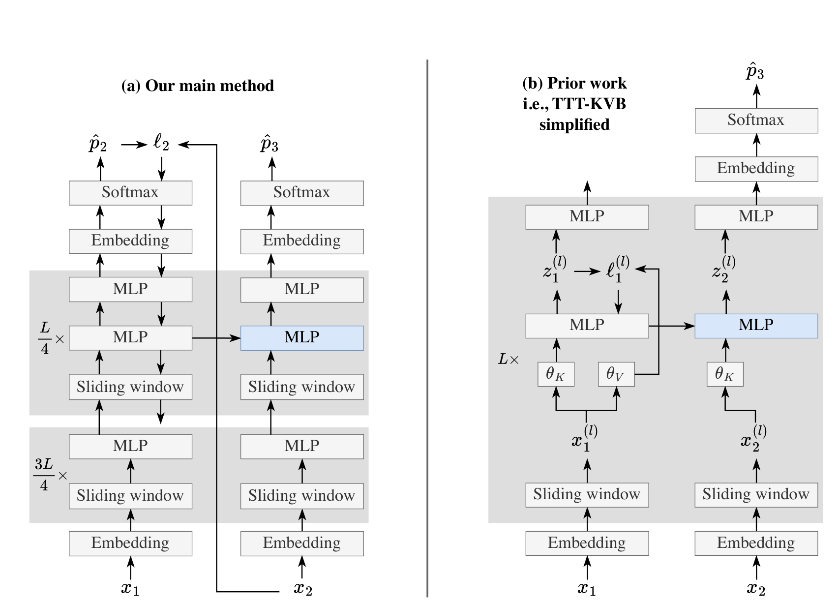
Figure 4. Paper Figure 3, cropped from PDF page 6. The diagrams contrast the end-to-end predictive objective with a local key-value binding objective. They show why replacing the inner loss can also simplify the adaptation structure.

Each adaptive block also receives a static MLP branch. Intuitively, one branch can retain reusable pretrained computation while the other changes with the document. The paper reduces MLP hidden dimensions across the network to preserve the overall parameter budget. Thus the comparison is not obtained by simply appending an unrestricted extra network to an otherwise identical baseline.

Why adapt late layers? Updating earlier layers forces differentiated inner learning to pass through more of the model and enlarges the mutable state. Later layers offer a more economical place to write context-dependent information. The ablation provides empirical support for the choice: in the 24-layer 760M configuration, six adaptive layers work well; reducing the number much further damages context scaling, while doubling it is not clearly better. This does not establish that early-layer adaptation is inherently useless.

A useful alternative would be a small low-rank adapter. It reduces per-session state, but also restricts the set of document-specific changes that the system can express. Another alternative is to adapt all MLPs with a first-order approximation to the outer gradient. That might reduce some training costs, but it changes the optimization and is not equivalent to the evaluated final design. These alternatives clarify the tradeoff without claiming that the paper has tested every variant.

7. Three algorithms and their information boundaries

The following pseudocode restates the mathematical method. It is not a report of inspecting the authors’ software. Details absent from the paper, such as a service’s policy for a final partial generation chunk, are left as explicit engineering decisions.

Algorithm 1. Causal prefill with adaptation

Input: context X, outer-trained W_init and phi, chunk size b
1. Set W <- a fresh per-sequence copy of W_init.
2. Initialize the bounded causal attention state.
3. For each observed chunk C, in temporal order:
   3.1 Predict the targets in C using W and phi.
   3.2 Enforce causal masking within C.
   3.3 Record the mean next-token loss before any update on C.
   3.4 Differentiate that loss with respect to fast weights W.
   3.5 Apply the inner update to W.
   3.6 Retain only the attention state allowed by the window.
4. Return the adapted W and the local attention state.

Line 3.3 separates evaluation from fitting. Scoring a chunk after optimizing on its own targets would leak the answers into the reported loss. During inference, the purpose of the gradient is to improve future predictions. During outer training, the sequence of such operations becomes part of the computation graph for learning the initialization and static parameters.

Algorithm 2. Outer training through inner learning

Input: a batch of independent training sequences
1. For each sequence, initialize its own fast weights at W_init.
2. Run causal chunk scoring and inner updates as in Algorithm 1.
3. Average the losses scored before their corresponding updates.
4. Differentiate this average through the inner update trajectory.
5. Accumulate outer gradients for W_init and static parameters phi.
6. Apply the outer optimizer update.
7. Discard per-sequence adapted states before the next sequence.

The reset is part of the statistical experiment: independent training documents do not silently share a continually changing state. Retaining one user’s adapted weights for another user’s document would change both the behavior and the isolation assumptions. Conversely, intentionally maintaining a persistent personal state would require an evaluation protocol beyond the document-level results reported here.

Algorithm 3. Generation with periodic adaptation

Input: the prefilled fast weights and local attention state
1. Generate new tokens causally with the current state.
2. Accumulate the newly generated tokens until one inner chunk is full.
3. Compute its causal next-token loss and update the fast weights.
4. Continue generation from the updated state.
5. Stop at the requested end condition.

The update in Algorithm 3 uses the model’s own generated continuation. That signal is not identical to an independently observed document. Errors or repetitive patterns may become part of the training signal. The paper evaluates generated text, but the algorithm alone does not prove that adaptation will always improve factuality or diversity. A production design must also decide how to handle cancellation, branching generation, incomplete chunks, and state disposal. These are consequences of the stateful method, not measured accomplishments of the paper.

8. Replacing key-value binding with the final task loss

An earlier family of TTT layers trains a local associative memory. A projected input becomes a key, another projection becomes a value, and a small function $g$ learns the binding. In simplified notation, the local objective is

$$\ell_t^{\mathrm{KVB}}(W) =\left\|g(\theta_K x_t;W)-\theta_V x_t\right\|_2^2. \tag{10}$$

The original formulation then reads the updated memory with a query projection, $g(\theta_Q x_t;W_t)$. The paper first simplifies this construction by using the pre-update weights and the key projection for the output. It next substitutes the entire network’s next-token objective for the local reconstruction objective, and finally changes the placement and structure of the adaptive MLPs.

Why should the objective matter? A local reconstruction loss trains the memory to preserve projected input information. The outer objective must make that information useful for language prediction indirectly. An end-to-end next-token inner loss uses the actual prediction error to decide what to write. It removes that particular surrogate-objective mismatch. It does not remove the mismatch between next-token prediction and a downstream task such as exact retrieval.

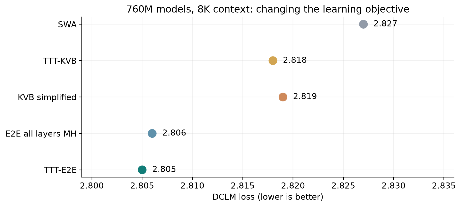
Figure 5. Redrawn from paper Table 1: 760M models on the reported 8K DCLM setting. The values are losses, with lower being better. The restricted horizontal range makes small differences readable; it is not a claim of a large multiplicative improvement.

The progression is informative. Sliding-window attention has loss 2.827; the original TTT-KVB has 2.818; the simplified KVB version has 2.819; an end-to-end version that still uses multi-head updates in all layers reaches 2.806; the final TTT-E2E reaches 2.805. The largest step in this particular sequence of ablations comes from changing the inner objective, while the final architectural simplification changes the loss only slightly.

This evidence supports the value of task-aligned adaptation in the tested setting. It is not a complete factorial experiment over all objectives, parameter counts, state sizes, and update placements. In particular, the final adaptive state contains 88M parameters versus 18M for the all-layers multi-head E2E intermediate model, approximately a fivefold difference. With a total parameter budget held comparable, the amount of state available to store the current document can still differ substantially.

The paper also reports 0.0086 versus 0.017 seconds per 1K tokens for the final E2E and all-layers multi-head E2E variants in the associated 760M comparison. This is a different model-scale comparison from the headline 3B result. Mixing the state size, loss numbers, and latency numbers from different tables into a single imaginary configuration would make the method look more precisely characterized than it is.

A structural reason for the state difference is that splitting a width-$D$ linear map into $H$ independent heads reduces the dense weight count from $D^2$ to approximately $D^2/H$. Low-rank restrictions can reduce it further. Moving from the all-layers multi-head E2E intermediate model to fewer ordinary MLPs changes both the optimizer’s computational pattern and the capacity of the state. Objective alignment and memory capacity therefore deserve separate attention in subsequent work.

9. Reading the scaling evidence

9.1 What was trained and what was tested

The paper studies model sizes from 125M through 2.7B parameters, commonly rounded to 3B in the discussion. The main data path is pretraining on DCLM with documents shorter than 8K removed, followed by long-context training on Books. The main loss evaluation uses held-out Books text. The headline model is reported as trained on 164B tokens.

Models evaluated at different target context lengths are not all the same checkpoint simply receiving longer inputs. They are separately extended to the target lengths from a pretrained checkpoint. This distinction is essential when interpreting a smooth context-scaling curve: it combines an architecture with a context-length training procedure. It does not by itself establish zero-shot extrapolation from an 8K-trained model to a 128K stream.

At the reported larger scales, TTT-E2E approaches full-attention predictive performance as context grows and outperforms the other constant-per-token-cost alternatives in the principal plots. Its advantage is not equally strong at every model or training-token scale. The study reports unstable long-context training for some small models, and trends that change with data and tokenizer choices. These observations narrow the empirical claim rather than invalidate it.

9.2 The ablations explain complementary components

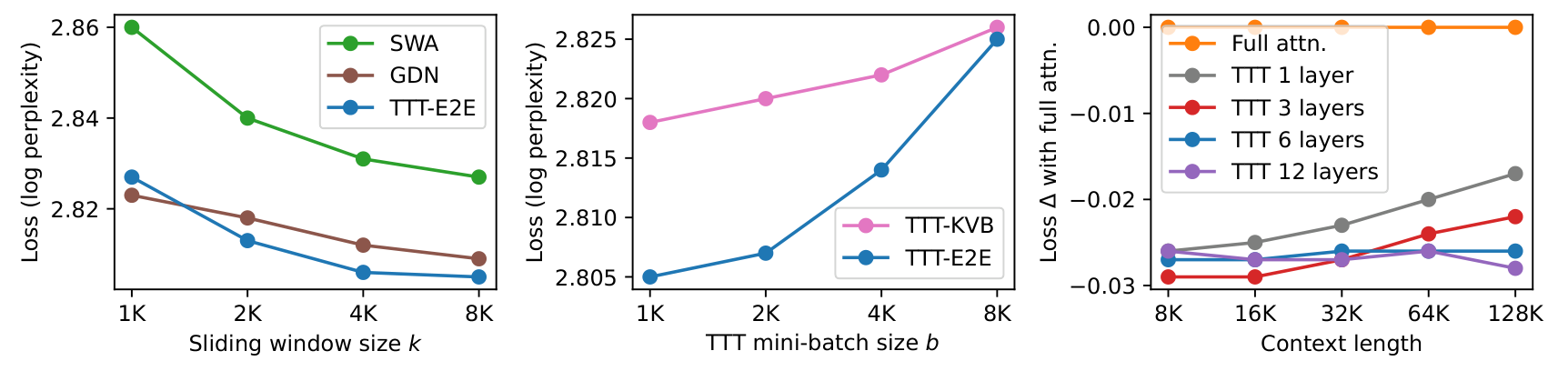
Figure 6. Paper Figure 4, cropped from PDF page 10. These experiments help explain why the final design combines an 8K local window, 1K inner chunks, and a limited set of adaptive layers. The curves are configuration-specific evidence, not a universal tuning rule.

The local window addresses information that is too recent to have reached the fast weights. The chunk size controls how often information is written. The number of adaptive layers controls the capacity and cost of that write mechanism. Reading these knobs together is more useful than presenting three disconnected best settings.

There are protocol details worth retaining. The layer-count ablation uses the 760M model, and its sequence batch is doubled across context lengths to improve stability. At the 8K pretraining length, an 8K window is already full attention within the sequence. The method can nevertheless gain from adaptation across 1K chunks; this is why the 8K comparison is informative about learning dynamics rather than about discarding distant attention connections.

The paper also examines a configuration in which the inner chunk covers the entire 8K sequence. With no useful within-sequence adaptation, the architectural variants achieve losses around 2.825 and 2.826, close to the full-attention baseline’s 2.827. That result is consistent with most of the gain requiring the adaptation-aware training procedure rather than simply an extra static branch.

9.3 Improvement before the first update is a different mechanism

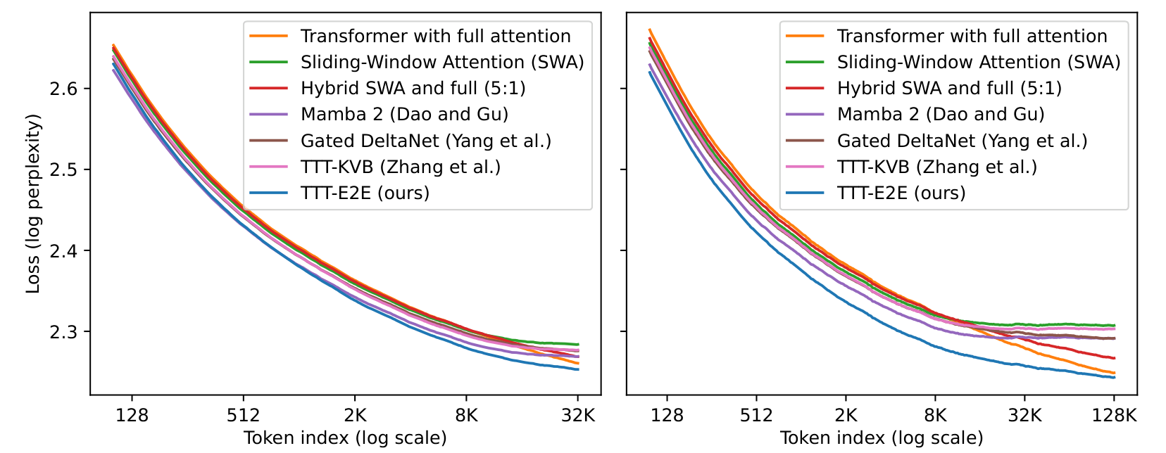
Figure 7. Paper Figure 6, cropped from PDF page 13. The 32K and 128K panels involve the relevant context-trained models. An early-position advantage can reflect a better learned initialization before the current sequence has supplied a full update chunk.

The position-wise curves are especially revealing. TTT-E2E can already have an advantage before the first 1K-token update has occurred. That early improvement cannot have been caused by an update on the current sequence. It must arise from what the outer training has learned: its initialization, static computation, or their joint organization.

Later improvements may combine that effect with adaptation to the current context. A plot of final loss alone does not separate the two. A particularly useful follow-up experiment would hold the trained checkpoint fixed and disable or shuffle its inner updates at evaluation. This is a proposed causal diagnostic, not a result supplied by this review. It would help estimate how much of the gain comes from learning to initialize versus learning from the current document.

10. Exact retrieval exposes the compression boundary

A next-token predictor can exploit a book’s style, recurring entities, topic, and local narrative structure without preserving every random string. Needle-in-a-haystack tests ask a different question: can a model reproduce a particular piece of information hidden in a long context? The paper’s results show a sharp distinction between these capabilities.

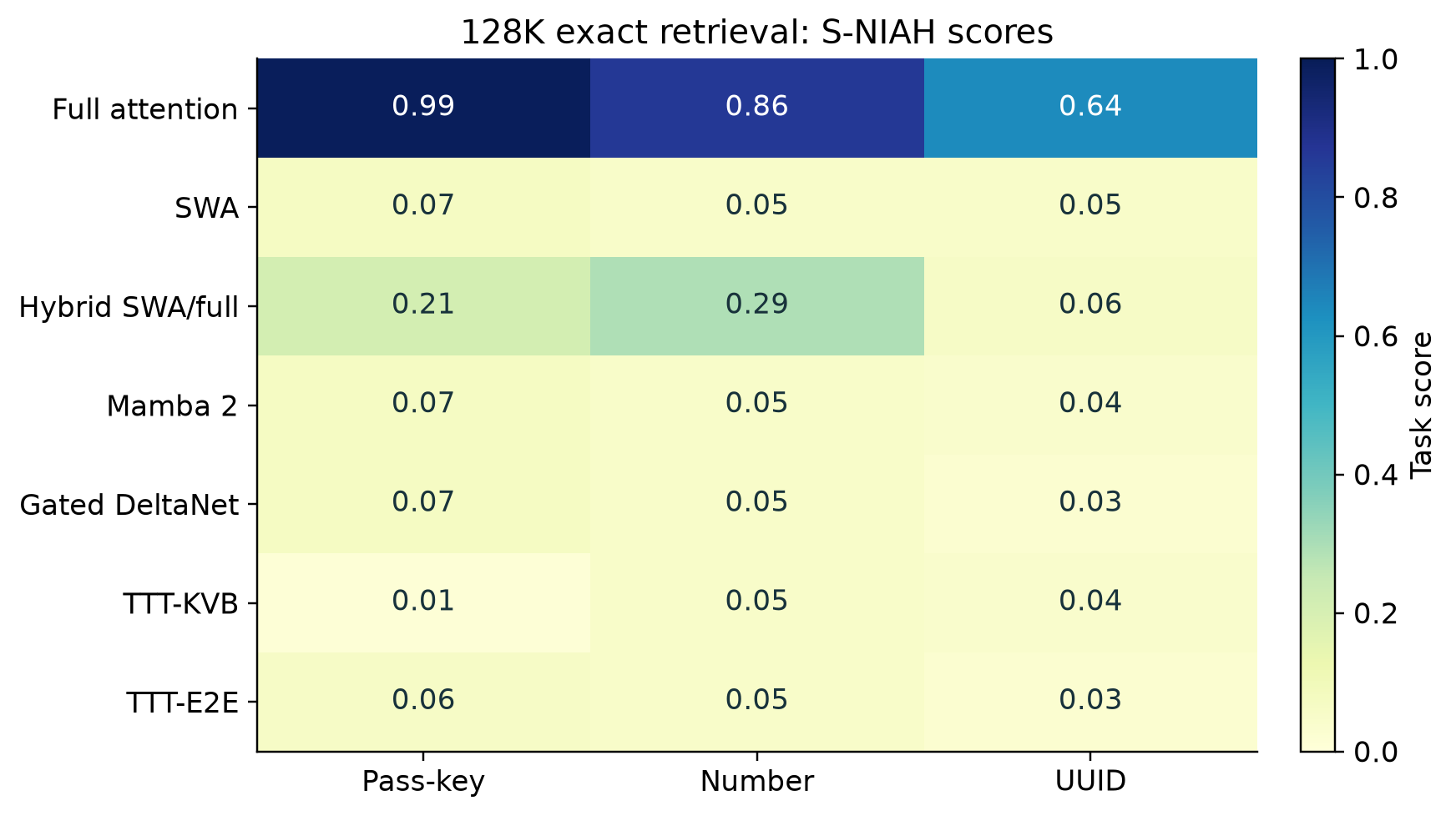
Figure 8. Redrawn from paper Table 2, using its 128K columns. The three single-needle tasks use a passkey, a number, and a UUID. Values are reported retrieval scores; these are not language-model losses.

At 128K, full attention scores 0.99, 0.86, and 0.64 on those three tasks. TTT-E2E scores 0.06, 0.05, and 0.03. Other compressed-state alternatives also struggle. The comparison prevents a broad claim that low predictive loss means comprehensive long-range recall.

The length trend matters as well. TTT-E2E’s passkey result declines from 1.00 at 8K to 0.46 at 16K, 0.24 at 32K, 0.13 at 64K, and 0.06 at 128K. The tested models were extended to 128K, then evaluated at these lengths. Good local retrieval is therefore compatible with weak retention beyond the direct attention window.

Why can this happen? The training objective rewards information according to its effect on future token prediction. An arbitrary UUID may have very little predictive utility until a later explicit query asks for that exact sequence. A finite mutable state is encouraged to compress, and the relevant training distribution may not teach it to reserve sufficient capacity for all such details. This is an interpretation of the objective and results, not a proof of which internal representation was learned.

The practical consequence is task-dependent. For document adaptation or topic-sensitive continuation, the loss improvements are meaningful. For legal citations, exact configuration values, identifiers, or source-grounded answers, explicit access to the original evidence remains important. A hybrid system could use adaptation for broad context and retrieval for exact details. That proposal follows from the complementary failure modes; this paper does not demonstrate the full hybrid product.

11. Efficiency means three different workloads

11.1 Prefill: bounded marginal cost, growing total work

The headline prefill comparison uses one H100 and holds the total number of tokens per batch at 128K. An 8K context therefore permits more sequences per batch than a 128K context. This is a controlled throughput-oriented setup. It is not identical to measuring single-request latency at every length or maximizing throughput independently for every architecture.

The reported 2.7-fold prefill speedup at 128K is useful evidence under that setup. The near-flat normalized curve means that processing another fixed-size portion of context costs approximately the same amount. With fixed model size, window $k$, and chunk size $b$, a schematic total cost is

$$C_{\mathrm{prefill}}(T) \approx T\,c_{\mathrm{local}}(k) +\left\lceil\frac{T}{b}\right\rceil c_{\mathrm{update}}(b). \tag{11}$$

Both terms grow linearly in $T$ for fixed $k$ and $b$. Dividing by $T$ yields a bounded average cost per token. Reading the whole document still takes longer when the document is longer. Full attention, in contrast, has a growing attention-interaction term, although its optimized kernels and parallelism can be highly competitive at moderate lengths.

11.2 Decode: the average hides periodic updates

For generation, tokens between update boundaries follow the sliding-window path. At a boundary, the model performs an adaptation step. An illustrative amortized expression is

$$\overline c_{\mathrm{decode}} \approx c_{\mathrm{token}}(k)+\frac{c_{\mathrm{update}}(b)}{b}. \tag{12}$$

This is an accounting identity under simplified stationary costs, not a measured decode benchmark from the paper. The authors discuss generation cost composition but do not provide a standalone decode-latency study comparable to the prefill plot. A streaming service should care about the delay at update boundaries as well as the average. Two methods can have similar mean time per token but very different pauses visible to a user.

Memory also has a serving dimension. The shared pretrained parameters are only part of a multi-session deployment. A useful conceptual budget is

$$M(S)\approx M_{\mathrm{shared}} +S\left(M_{\mathrm{fast}}+M_{\mathrm{local\ cache}}+M_{\mathrm{update\ work}}\right), \tag{13}$$

for $S$ simultaneous independent sessions. Actual peak memory depends on scheduling, precision, gradient buffers, and whether workspace can be reused. If an update rule stores extra optimizer state, it also belongs in the per-session or scheduled workspace budget. The formula does not assume that the paper uses any particular stateful inner optimizer.

Unlike an ever-growing full attention cache, these terms can remain bounded with respect to document length. Yet bounded is not the same as small. The 88M fast-state parameters in the 760M comparison would occupy approximately 176MB at two bytes each before gradients or other workspace. That calculation illustrates a capacity concern; it is not a measured serving-memory result or a claim about the 3B configuration.

11.3 Training: learning the update rule is expensive

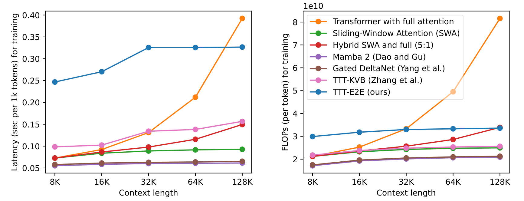
Figure 9. Paper Figure 8, cropped from PDF page 16. Training-latency measurements use H200 in this comparison, whereas the main prefill comparison uses H100. Training, prefill, and decode should not be merged into a single speed claim.

The paper reports approximately 3.4-fold slower training at 8K but 1.2-fold faster training at 128K relative to its Transformer comparison. This reversal follows the changing balance between full attention’s growing cost and the costs of differentiating through updates. A long-context inference benefit does not imply that pretraining the method is uniformly cheaper.

Higher-order derivatives interact with the available kernels. The paper discusses a lack of support for the required derivatives in a fused attention path and the use of checkpointing through time. Checkpointing trades stored activations for recomputation; its overhead can increase with the unrolled trajectory. Consequently, nearly flat estimated operation counts per token need not translate into flat measured training latency.

These measurements motivate custom kernels and alternative initialization strategies, but those possibilities should remain future work. The reported models and baselines also use different software frameworks in parts of the study. The paper describes efforts to improve baseline kernels. For an application decision, one should still compare the complete stack under equal hardware, memory, token budget, and wall-clock constraints. This review does not run such a benchmark.

12. Limitations of the evidence

Scale and length are finite. The main empirical envelope reaches roughly 3B parameters and 128K tokens. An asymptotic argument supports bounded per-token work when the window and state are fixed, but it does not establish stable quality on arbitrarily long streams. Update counts, content shifts, and retained information can all change outside the evaluated range.

The data emphasizes sustained text. The path through filtered DCLM and Books provides a natural setting for recurring linguistic structure. It does not comprehensively represent tool logs, interleaved conversations, multilingual mixtures, source-code repositories, or long documents where one rare exact detail dominates the task. A method that learns a book’s regularities may need different objectives or safeguards in these settings.

Predictive loss and generation quality are related but distinct. The paper evaluates generated continuations with an external Qwen3-8B-Base language model, using 8K prefill and 8K generation across 512 sequences. Sampling uses temperature 1, top-p 0.95, and repetition penalty 1.1; the authors also describe a small manual inspection. External-model likelihood is a proxy, not a factuality or instruction-following guarantee. Repetition controls matter because predictable repetition can look good to a likelihood metric.

The retrieval gap is substantial. The needle results are a direct observed limitation, not merely a theoretical concern. Strong predictive compression should not be advertised as exact memory. The paper does not establish broad downstream question answering, instruction-following, or agent performance after supervised or reinforcement-learning post-training.

Serving remains incompletely measured. Prefill throughput is reported, while concurrent-session capacity, branching requests, tail latency around update boundaries, and sustained decoding need fuller evaluation. The fixed-total-token batching rule is important context for the prefill advantage.

Optimization can be fragile. Restricted update locations, chunk-size choices, small-model instabilities, and sensitivity to training details all indicate that end-to-end inner learning is not a costless replacement for attention. The paper reports encouraging scaling, but not a universal recipe for every model family.

13. Critical analysis

13.1 The strongest contribution is a change in what is optimized

My reading is that the important conceptual move is not simply storing a document in weights. Recurrent models already store history in state, and gradient-based memory predates this paper. The stronger contribution is to let the final language-prediction objective determine both what the inner loop writes and how the outer loop prepares the network to be written into.

The controlled progression from KVB to E2E supports that interpretation. Nevertheless, the larger adaptive state and architectural reorganization are part of the actual system. A decisive capacity-controlled study would compare objectives at matched mutable-state size and update cost, then report predictive quality, exact recall, and training expense together. The current results justify serious attention, while leaving this attribution question open.

13.2 Initialization quality and online learning should be separated

The early-token advantage is easy to overlook. It means that some benefits are present before the current document changes the weights. That is valuable: an adaptation-aware outer objective can apparently improve the starting model as well as its learning trajectory. It also means that attributing the entire gap to memorizing the current context would be incorrect.

A useful evaluation matrix would compare the same trained initialization with normal updates, disabled updates, shuffled chunk order where meaningful, and updates on unrelated context. Predictions must remain causally scored in every condition. These are proposed diagnostics, not experiments conducted here. Their purpose would be to distinguish helpful current-context adaptation from improvements already encoded by outer training and from harmful sensitivity to irrelevant text.

13.3 Compression deserves a task-specific contract

The retrieval result suggests that a deployable adaptive memory should state what it is expected to retain. Topic and style adaptation tolerate lossy summaries. Quoting an identifier does not. A system that combines an adaptive predictor with an explicit evidence store can assign these responsibilities separately, but it then inherits retrieval cost and state-management complexity.

One might add an auxiliary retention objective or train on tasks that reward delayed exact recall. That could improve the missing capability, or it could reduce predictive gains and consume additional state. The paper does not resolve this tradeoff. The correct conclusion is that the objective selects the kind of memory being learned, not that a sufficiently long context length automatically supplies every kind of memory users want.

13.4 Self-generated updates need a quality argument

During document ingestion, the observed next token provides an external signal. During free generation, the model trains on its own outputs. These regimes should not be assumed equivalent. A mistaken entity, repetitive phrase, or abrupt topic shift can enter the update stream. Outer training may make the learner robust to familiar patterns, but robustness to all generated errors is not established.

Potential policies include updating only on externally observed text, gating high-loss chunks, or keeping recoverable state checkpoints. Each would alter the learning distribution and could remove useful adaptation. They should be evaluated as new systems choices. This is particularly relevant for agents that mix user input, tool outputs, and their own reasoning: those sources carry different kinds of evidence.

13.5 A fair systems question includes the training bill

For a one-time research demonstration, a faster long-context prefill can be compelling even if training is expensive. For a deployed family of models, the decision depends on how much inference is amortized over each trained checkpoint. A model with a large training premium might still be worthwhile for repeated very long workloads, while being unattractive for short contexts or low utilization.

The missing measurements are concrete: identical-quality checkpoints at matched training wall time; peak per-session mutable memory; concurrent throughput; decode tail latency; and quality under uninterrupted streams longer than the training sequence. None is required to acknowledge the reported result, but all matter before treating the method as a general serving replacement.

14. Conclusion

TTT-E2E offers a coherent route to long-context language modeling: local attention preserves immediate detail, gradient updates compress older context into a fixed-size adaptive state, and outer training makes those updates part of the prediction problem. Its strongest reported evidence combines near-full-attention predictive loss with a 2.7-fold prefill speedup at 128K in the stated 3B/H100 setup.

The paper also makes the boundary visible. Exact long-range retrieval remains weak, training can be more expensive, and decoding or multi-session serving needs further measurement. The useful lesson is to evaluate a memory mechanism by the information its objective teaches it to retain. TTT-E2E is an encouraging predictive memory, with a clear agenda for testing where that memory is sufficient and where explicit access to the original context is still needed.

References and figure provenance

1. Arnuv Tandon et al. End-to-End Test-Time Training for Long Context. arXiv:2512.23675v2, 31 December 2025. Paper and version history; full PDF. This review reads the full 29-page document, including Appendices A–D.
2. Official project and official code resource. These links are provided as resources; the analysis above is based on the paper and its appendices.