SICA: When a Coding Agent Becomes Its Own Next Engineer

Review date: October 5, 2026
Author: Zhongzhu Zhou
Paper reviewed: A Self-Improving Coding Agent
Paper authors: Maxime Robeyns, Martin Szummer, Laurence Aitchison
arXiv: 2504.15228v2, May 16, 2025

1. The claim I want to understand

A language model can write code that changes the software around a language model. That observation sounds almost trivial until the surrounding software is also responsible for choosing and carrying out the next change. SICA turns this feedback loop into an experiment. It keeps earlier agent programs and their results in an archive, selects the program with the highest measured utility, and asks that agent to create another version. The foundation model weights remain fixed. The editable object is the program that manages prompts, tools, sub-agents, context, and execution.

My main takeaway is that SICA makes a concrete case for learning through changes to an agent’s working environment. Some of the useful changes are ordinary engineering: smaller file edits, better symbol lookup, more economical observations, and more deliberate routing. Their value comes from placing them inside a repeated propose-and-evaluate loop. A successful tool improvement can help the agent solve external coding tasks and also help it edit its own framework during a later iteration.

The headline result needs its denominator. The paper reports a rise from 17% to 53% on a fixed random 50-question subset of SWE-bench Verified. These are the iteration 0 and iteration 14 entries in Table 1. Iteration 15 reports 51%. The study is not a full SWE-bench Verified leaderboard evaluation. Its five-minute task timeout and resource-sensitive selection also define a different operating point from an unconstrained coding agent. I will retain these qualifications when interpreting the gain.

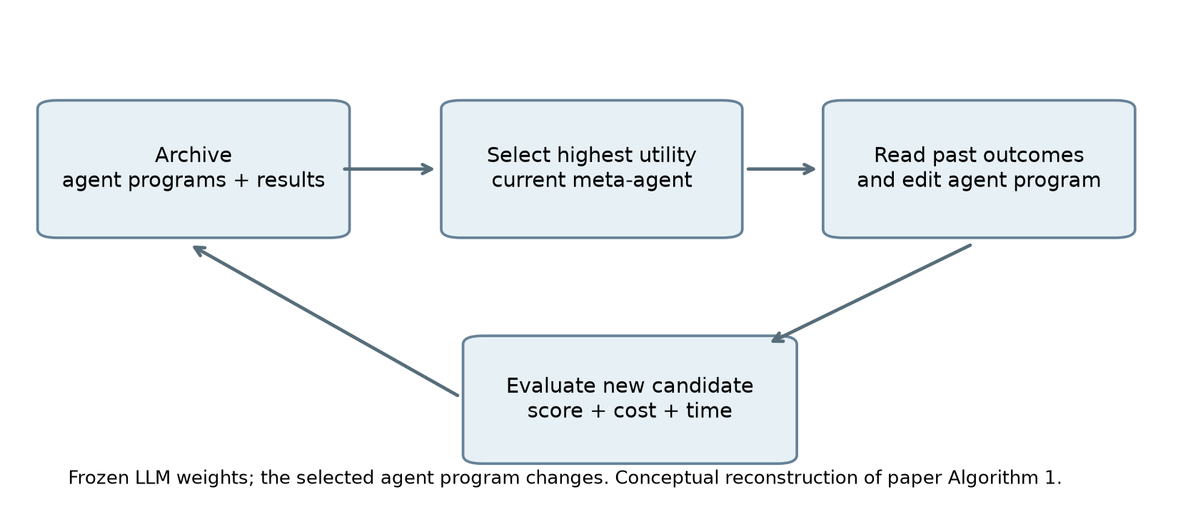
Figure 1. My reconstruction of paper Algorithm 1 and Section 3. The archive supplies both evidence and the next editor. The model weights remain fixed, while the agent program used for subsequent editing can change.

There is an equally useful negative result. A second experiment on AIME 2024 and GPQA Diamond finds little improvement from the additional scaffold. An already strong reasoning sub-agent often does the substantive work; extra orchestration can contribute overhead or disrupt that work. This makes the paper a study of where agent engineering helps, rather than evidence that more recursive structure always produces more intelligence.

The discussion below is based on the complete 18-page v2 paper, including its prompts, traces, function-calling description, and change log. I distinguish the paper’s numerical observations from my explanatory calculations and proposed experiments. The figures labeled as reconstructions use reported numbers; the utility heatmap and experimental-design diagram are explanatory artifacts, not reproduced experimental outcomes.

2. Prerequisites: what exactly can learn?

2.1 A model, an agent program, and a running process

Three objects are easy to conflate. A model with parameters $\theta$ maps context to generated tokens. An agent program $g$ turns those tokens into tool calls, observations, and future contexts. A running process also contains temporary state: open files, previous messages, pending work, and the task’s partial solution. In SICA, improvements persist mainly in $g$, rather than in model parameters or one conversation’s temporary state.

For exposition, I represent one task execution as a trajectory $z$ and its returned artifact $y$:

$$z\sim P(z\mid x,g,\theta),\qquad y=\operatorname{Return}(z),\qquad \theta\text{ fixed}. \tag{1}$$

Changing $g$ can change performance even with identical $\theta$. A tool that returns a precise symbol definition may avoid ten unproductive searches. A patch editor may replace a large generated file with a small edit. A router may call a capable reasoning model directly. Each changes the distribution of observations and future decisions available to the same underlying models.

This is a persistent form of adaptation, but it is not gradient-based training of the foundation model. A new agent program can be saved and reused for another task. Conversely, one useful reflection that exists only in the current conversation disappears when that conversation ends unless it is stored in a reusable form. SICA’s archive gives program changes a durable representation and connects them to measurements.

2.2 Task performance and improvement performance

Being a good coding agent is related to being a good agent designer, but the relationship is not automatic. A task solver may be excellent at changing application code and poor at selecting a useful architectural intervention. A meta-improvement step has at least three burdens: diagnose a failure pattern, propose a change with positive expected value, and implement it without damaging other behavior. Higher benchmark utility directly measures only the downstream solver, not all three meta-level abilities.

Let $g_i$ be an archived agent, $\widehat U_i$ its measured utility, and $H_t$ the archive at time $t$. My shorthand for the paper’s selection rule is

$$j_t=\arg\max_{i\leq t}\widehat U_i,\qquad g_{t+1}\sim Q(\,\cdot\mid g_{j_t},H_t,\theta). \tag{2}$$

Here $Q$ denotes the behavior of the selected agent when asked to improve the agent system. It is not a separate trained probability model introduced by the paper. Equation (2) simply makes the dependency visible: the program selected for task quality also influences the next proposal. To establish a recursive advantage, we would like evidence that improving the selected program improves $Q$, not merely evidence that the new downstream task score increased.

SICA operationalizes self-reference more directly than an arrangement with a permanently fixed meta-agent editing a separate target agent. This is the paper’s contrast with ADAS. I would avoid treating that terminology as a binary definition of all self-improvement research. The important engineering question is which component changes, which measurements select it, and which parts of the search remain externally specified.

2.3 Search uses a noisy evaluator

An archive is a collection of candidate systems and observations, not a proof that its winner is best. The measured score includes finite task sampling, stochastic model outputs, API timing, and possibly infrastructure variation. Selecting the maximum observed value amplifies favorable noise. A failed candidate can still contribute diagnostic evidence; a winning candidate can still have been lucky.

This is why a best-so-far curve is insufficient on its own. Define the recorded incumbent utility as

$$M_t=\max_{0\leq i\leq t}\widehat U_i \quad\Longrightarrow\quad M_{t+1}\geq M_t. \tag{3}$$

The monotonicity is a property of taking a maximum. It does not prove that every child improves, that the incumbent generalizes, or that the search will continue finding useful changes indefinitely. The raw candidate curve and the tasks on which it is measured are necessary companions to that appealing red line.

3. The starting agent is already a designed system

3.1 Tools and delegation create the search substrate

The initial system is more substantial than a bare language model with a terminal. Section 3.1 describes tools for opening and closing files in context, overwriting files, executing shell commands, using a calculator, submitting a benchmark answer, and returning or exiting from sub-agent calls. An archive-analysis tool exposes high-level statistics from earlier iterations. The initial agent therefore starts with both editing capabilities and a way to inspect its own history.

The paper includes a main routing agent plus coding, problem-solving, and reasoning sub-agents. A sub-agent accepts arguments and returns a string, much like a tool. The abstraction supports decomposition, but it also has a context-management role: detailed child work can disappear from the parent’s active context and be replaced by a concise returned result. This reduces the need for one long conversation to retain every intermediate observation.

That benefit has a cost. A summary can omit the exact file location, a failed assumption, or the distinction between a test passing and a hypothesis being plausible. A parent that receives only a confident summary may repeat work or accept an incorrect conclusion. Delegation should therefore be evaluated through successful completion under the resource budget, not through the number of specialized roles a system has created.

3.2 Context layout is part of the algorithm

The paper separates system context, core context, and the growing assistant history. System context defines the role, available tools, sub-agents, and execution instructions. Core context contains the task, open files, and a directory view. The history contains model messages, tool observations, sub-agent outputs, and overseer notifications. This arrangement affects both what the model sees and what can be reused by the inference service.

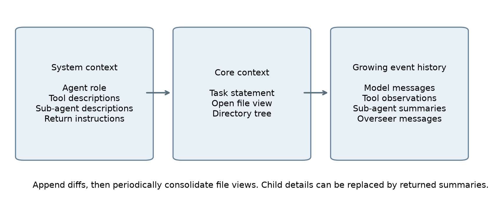
Figure 2. An original diagram based on paper Figure 2 and Section 3.1. File views and observations are part of the agent’s effective state; the written system prompt alone does not describe the whole method.

The authors append file edits as diffs and periodically consolidate the accumulated changes into the file view. Appending usually preserves more of an existing prefix than repeatedly replacing early context. That can improve cache reuse, but the benefit competes with freshness. A long list of diffs can force the model to reconstruct the current file mentally. Consolidation simplifies the representation while changing more of the prefix.

A useful mental model is a materialized view plus an update log. The view is easy to inspect but expensive to refresh; the log is cheap to append but grows harder to interpret. The right consolidation interval depends on file size, edit frequency, context length, and the provider’s caching behavior. SICA makes this engineering choice editable. It does not derive an optimal interval or establish that every increase in cached-token fraction is caused by a particular context change.

3.3 The overseer has a different view of progress

The initial agent also includes an asynchronous LLM overseer, called every 30 seconds by default or on important events. It sees a summarized call graph and event stream, including tool calls and agent activity. It can send a steering message or cancel a badly stalled execution. This allows one component to notice repetition across child calls that an individual child may not see.

I read the overseer as a progress-control mechanism with imperfect information. It can interrupt a genuine loop, but it can also interrupt a legitimate slow operation. Its own model calls consume resources. A healthy experimental comparison would measure successful interventions, false cancellations, and overhead. The paper describes the mechanism and provides its prompt; it does not provide a comprehensive causal decomposition of the overseer’s contribution.

The appendix also warns about a subtle process-state issue during self-editing: changing files on disk does not magically replace objects already loaded by a running process. Its overseer prompt directs the agent toward testing the new agent in a separate execution or using an explicit test script. The conceptual lesson is to keep “the program being edited” distinct from “the process currently doing the editing.” No special theory of self-reference removes this ordinary software boundary.

3.4 Function calls are an interface contract

Appendix C describes unconstrained XML-formatted generations whose closing tags act as stop tokens. The runner detects the stop reason, parses a tool name and arguments, dispatches the tool, and returns an observation. The authors prefer this representation partly because it avoids JSON string-literal escaping for large file contents.

This is a design tradeoff rather than a guarantee of correctness. Delimited text still needs parsing, validation, and an unambiguous termination convention. A constrained format or a provider’s native function interface may reduce some malformed-call cases but may constrain portability or expressiveness. The paper’s contribution is the adaptable agent system; one should not attribute the entire experimental gain to XML versus another serialization format without a controlled comparison.

4. Deriving the resource-aware utility

4.1 Normalize the quantities before adding them

A benchmark score is dimensionless, a cost is measured in dollars, and elapsed time is measured in seconds. Adding the raw values would be meaningless. The paper first expresses expense and time as fractions of reference budgets. Write task score $p\in[0,1]$, dollar cost $c\geq0$, and elapsed time $t\geq0$. The reference values are $C=10$ dollars and $T=300$ seconds.

Define two efficiency terms:

$$e_c=1-\min(1,c/C),\qquad e_t=1-\min(1,t/T). \tag{4}$$

At zero cost or zero time the corresponding term is one; at the reference limit it is zero. Beyond that limit the clipped term stays zero. This clipping prevents an arbitrarily expensive run from making the base utility arbitrarily negative. It does not by itself enforce a hard cost cancellation. The explicit timeout is described separately.

The paper assigns half of the total weight to task score and one quarter to each efficiency term:

$$U=0.5p+0.25e_c+0.25e_t. \tag{5}$$

For nonnegative inputs, every term lies between zero and its weight, so $0\leq U\leq1$. A zero-score run can still receive efficiency credit. That is a deliberate implication of additive utility. It makes rapid inexpensive failures comparable to slower successful runs, which may be reasonable in some applications and unacceptable in others.

4.2 The exchange rate hidden in the weights

Below the clipping limits, substitute Equation (4) into Equation (5), expand the brackets, and collect constants:

$$\begin{aligned} U&=0.5p+0.25(1-c/10)+0.25(1-t/300)\\ &=0.5p+0.5-0.025c-t/1200. \end{aligned} \tag{6}$$

Now compare two runs in that same region. The constant cancels, leaving

$$\Delta U=0.5\Delta p-0.025\Delta c-\Delta t/1200. \tag{7}$$

An extra dollar must be compensated by a five-percentage-point increase in score if time stays fixed. An additional 60 seconds requires a ten-percentage-point increase if cost stays fixed. These are calculations implied by the selected weights, not universal economic exchange rates. Different API prices or product latency needs would make different weights sensible.

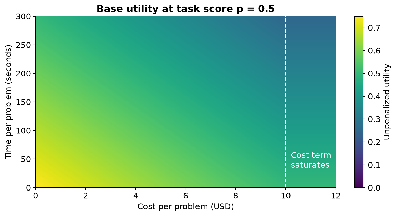
Figure 3. My calculation from the paper’s utility at a fixed task score of 0.5. The cost contribution saturates at USD 10. This depicts base utility before the timeout multiplier; it is not an experimental heatmap.

A concrete example makes the ranking less abstract. Candidate A scores 0.50, costs USD 2, and takes 120 seconds; its utility is 0.60. Candidate B scores 0.54, costs USD 3, and takes 150 seconds; its utility is 0.57. B has the better score, but A is preferred by this particular objective. The example is invented for arithmetic explanation. Neither candidate is an observed SICA iteration.

4.3 Timeout creates an additional discontinuity

The paper halves base utility after a timeout, using a penalty parameter of 0.5:

$$U_{\mathrm{final}}= \begin{cases} 0.5U,&\text{if the run times out},\\ U,&\text{otherwise}. \end{cases} \tag{8}$$

This is more than a gradual preference for faster answers. A run just before the deadline and one that times out can receive sharply different final utilities even when their partial work is similar. For an illustrative score of 0.5 and cost of USD 2, a completed run at 299 seconds has utility about 0.4508. At the 300-second boundary, if the run is classified as timed out, the same base quantities give final utility 0.225. This is an explanation of the rule, not a claim about the runner’s exact event-order convention.

The discontinuity creates strong incentives to remove operational friction. If slow file overwrites regularly prevent otherwise feasible fixes from finishing, an efficient patch tool can improve both score and time. This offers a plausible mechanism for the large coding improvement. It also explains why the result should not be read as a pure measure of newly acquired abstract reasoning ability.

The score is used for archive selection and as information for the next improvement step. It is not differentiated through to update model weights. “Reward” in this setting therefore has a narrower operational meaning than the training reward in policy-gradient reinforcement learning.

5. Reading the algorithm without hiding its bookkeeping

Algorithm 1. Self-referential improvement, with explicit measurements

The following is explanatory pseudocode for Section 3. It makes candidate evaluation explicit; it is not a verbatim transcription of the paper’s compact indexing.

1. Create the initial agent program g0 and a fixed benchmark set B.
2. Evaluate g0; archive its task results, resource use, and utility.
3. For each allowed improvement attempt:
4.     Select an archived agent with the highest measured utility.
5.     Give that agent the improvement task and archive evidence.
6.     Let it diagnose, propose, and construct a candidate program.
7.     Evaluate the candidate under the same benchmark conditions.
8.     Archive its program, observations, and measured utility.
9. Report the final candidate and the best measured incumbent separately.

The final line is a reporting clarification. The paper’s Algorithm 1 returns the final generated agent, while its selection rule repeatedly uses the best archived agent. These are different objects. Its abbreviated loop evaluates the current agent before generating the next, so an implementation or experimental report must also make the final candidate’s evaluation explicit. I do not infer missing experimental steps from the pseudocode alone.

Retaining an unsuccessful candidate does not mean choosing it as the next editor. SICA’s described rule greedily chooses the highest-utility archived program. The archive still carries negative evidence and earlier designs, but this is different from an explicitly diversity-seeking parent sampler. An archive can support broad reasoning while the actual parent-selection rule remains narrow.

This distinction matters when comparing SICA with yesterday’s DGM reading. Both allow editable agent programs and retain history. SICA’s central description selects the current best program as the meta-agent; DGM emphasizes an archive and exploration over multiple lineages. These are method differences worth investigating. The papers’ headline numbers come from different task populations and budgets, so they cannot decide which method is superior.

Algorithm 2. Calculate utility for a single task run

This pseudocode spells out Equations (4)-(8). The paper’s table contains aggregate measurements, which must not be silently substituted for individual observations.

1. Read normalized task score p, cost c, elapsed time t, timeout flag z.
2. Compute cost efficiency ec = 1 - min(1, c / 10 dollars).
3. Compute time efficiency et = 1 - min(1, t / 300 seconds).
4. Compute base utility u = 0.5*p + 0.25*ec + 0.25*et.
5. If z is true, set final utility v = 0.5*u; otherwise v = u.
6. Retain p, c, t, z, and v together for subsequent aggregation.

Why retain the raw components? The clipping and timeout multiplier are nonlinear. In general, averaging the final task utilities is not equivalent to applying the utility function to averaged score, cost, and time. For example, two costs of USD 0 and USD 20 have mean USD 10. Their mean clipped cost efficiency is 0.5; computing efficiency from their mean gives zero. The extreme numbers are illustrative, but the mathematical problem is real.

The paper’s Table 1 reports benchmark-level scores and cross-benchmark resource averages. It does not supply enough information to reconstruct every candidate’s exact aggregate final utility, timeout pattern, or confidence interval. Accordingly, I redraw the raw reported components and do not manufacture an exact utility series from their means.

Algorithm 3. Read an archive as evidence, not just a ranking

This is my analytical procedure for understanding the paper’s loop and traces, not an additional experiment carried out by the authors.

1. Find tasks where the incumbent failed or exhausted its budget.
2. Separate locating, editing, reasoning, and execution bottlenecks.
3. Compare successful and failed traces for the same bottleneck.
4. State one change and the mechanism by which it should help.
5. Identify tasks or resource terms that the change could harm.
6. Compare the next measured candidate with the relevant predecessor.
7. Keep a causal hypothesis separate from the observed score change.

Appendix B offers a useful example of this workflow. An archive-explorer sub-agent compares iterations and success/failure cases, then returns a proposed direction. A coding sub-agent develops the change, and another coding sub-agent subsequently checks it in a separate pass. This is a reported trace illustrating the intended process. It is not a frequency estimate for how often all iterations followed the same sequence, nor proof that the chosen change caused the later score movement.

6. Experimental design and the populations behind the numbers

6.1 Four tasks measure different abilities

The main experiment combines four benchmark categories. File editing measures how closely an edited file matches a target version constructed from repository history. Symbol location asks for the file, line, and column defining a referenced symbol. SWE-bench Verified tests repository-level issue resolution. LiveCodeBench contains competitive-programming-style tasks with a stronger algorithmic component.

The two synthetic tasks are useful probes of the agent’s mechanics. A poor file-editing interface can be detected directly rather than only through a failed end-to-end repository task. At the same time, file similarity is not identical to semantic correctness, and symbol-location labels may be unreliable when the target belongs to a missing external library. The authors explicitly acknowledge data-quality problems in the symbol benchmark. A low score can therefore mix agent limitations with defects in the task specification.

The paper selects 50 fixed random SWE-bench Verified questions and 50 random LiveCodeBench questions. Most agents use Claude 3.5 Sonnet v2; the reasoning sub-agent uses o3-mini. This mixed-model design matters. A score belongs to the whole configured system, not to Sonnet alone. Improving routing to a stronger component can produce a useful system gain without demonstrating that the weaker model acquired the stronger model’s internal capabilities.

The 15-iteration run is reported to cost approximately USD 7,000 in API usage. That figure describes the search run. It is distinct from the per-problem dollar costs in Table 1, and it should not be treated as the price of answering one benchmark question. A production decision would need the search expense, maintenance effort, and deployment volume as well as the final inference cost.

6.2 What Table 1 actually shows

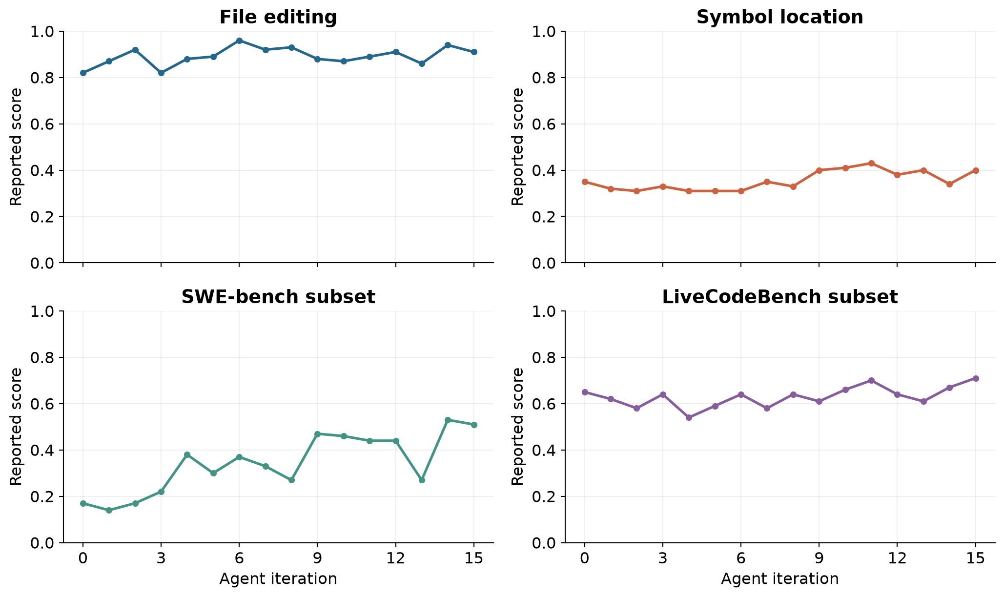
Figure 4. All 16 rows of paper Table 1 redrawn from the published rounded values. Scores are not uniformly improving. The SWE-bench and LiveCodeBench panels refer to the paper’s selected subsets; these curves are not full-benchmark leaderboards.

The most visible improvement is SWE-bench: 0.17 at the initial agent, 0.53 at iteration 14, and 0.51 at iteration 15. The increase to the peak is 36 percentage points. It is approximately 3.12 times the initial score, but the absolute gain is the clearer description because a small baseline makes relative ratios look dramatic. A ratio does not tell us which classes of repository problems became solvable.

File editing rises from 0.82 to 0.91 at iteration 15, with an earlier peak of 0.96. Symbol location rises from 0.35 to 0.40 at the final iteration, with a peak of 0.43. LiveCodeBench changes from 0.65 to 0.71 at the final iteration; it temporarily drops as low as 0.54 at iteration 4. A useful overall system can still regress on an individual task category.

Table 1 prints values such as 0.17 and 0.53 even though the selected SWE-bench set contains 50 questions. A single deterministic binary evaluation on 50 tasks would move in increments of 0.02. Without additional per-run aggregation details, these printed decimals do not justify inventing exact solved-task counts or a binomial confidence interval. I preserve the reported scores rather than reverse-engineering fictional counts from them.

This is not a reason to discard the result. It is a reason to separate the reported mean from a stronger statistical reconstruction. Per-instance outcomes, repeated-seed counts, and aggregation conventions would be needed for a faithful uncertainty analysis. The paper’s plotted confidence intervals should be read as its reported intervals; my redraw of Table 1 deliberately adds no new bands.

6.3 Cost and speed improve unevenly

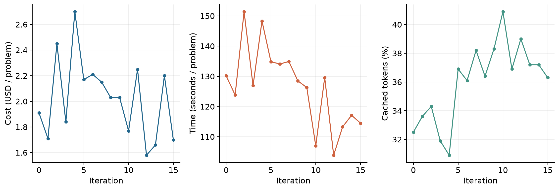
Figure 5. Mean per-problem cost, elapsed time, and cached-token percentage from paper Table 1. These resource statistics average across benchmark problems; they are not specific to the SWE-bench subset.

At iteration 0 the mean cost is USD 1.91 and mean time is 130.2 seconds. At iteration 15 the corresponding values are USD 1.70 and 114.5 seconds. Arithmetic on the rounded table entries gives about an 11.0% cost reduction and a 12.1% time reduction. Meanwhile the reported token volume increases from 0.24 million to 0.30 million per problem. Fewer dollars therefore does not simply mean fewer tokens.

Cached-token share, model mix, the balance of input and output tokens, and the pattern of repeated calls can all affect cost. The table alone does not isolate which factor explains the price difference. Cached-token percentage changes from 32.5% to 36.3%, but peaks at 40.9% at iteration 10. That observation supports paying attention to context structure without proving a one-variable causal explanation.

Iteration 14, which supplies the 53% SWE-bench headline, has mean cost USD 2.20 and time 117.1 seconds. Its cost is higher than the initial USD 1.91. It is therefore inaccurate to combine the peak accuracy at iteration 14 with the cheaper final cost at iteration 15 and describe them as one measured agent. Keeping the row identity attached to every number prevents an overly favorable synthetic result.

6.4 The cheapest agent, fastest agent, and best solver differ

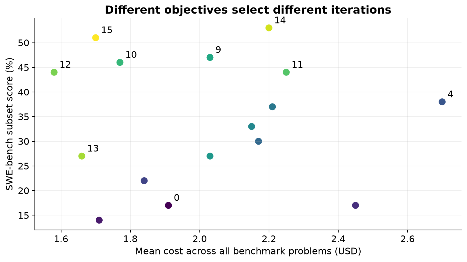
Figure 6. Table 1’s SWE-bench score plotted against its cross-benchmark mean cost; labels are iteration numbers. The axes use different task populations, so this is a way to compare recorded dimensions, not a SWE-specific cost-effectiveness frontier.

Iteration 12 has the lowest reported mean cost, USD 1.58, and the lowest mean time, 103.9 seconds. Its SWE-bench score is 0.44, not the maximum. Iteration 15 has the strongest reported LiveCodeBench score. Iteration 6 has the strongest file-editing score. No single row dominates every criterion in the published table.

A practical system can retain several artifacts for different deployment conditions. A latency-sensitive workflow might prefer one version; a difficult repository repair might prefer another. That would be an extension to the decision policy, not a result established by the paper’s scalar selection rule. The scalar utility is convenient because it creates a single winner, but it embeds a choice about which tradeoffs are acceptable.

7. What changed, and why might it help?

7.1 Efficient editing removes repeated output work

Appendix D records changes involving smart editing, faster overwrite operations, diff-based strategy selection, input normalization, and file-state tracking. The common mechanism is to reduce the amount of text and coordination required for a small code change. Rewriting a whole large file spends output tokens reproducing unchanged content and creates more opportunities to damage surrounding code.

A patch-based alternative can localize the intended modification. That introduces its own failure boundary: a patch may target stale content, ambiguous text, or the wrong occurrence. Input normalization and file-state tracking address related interface problems. An efficient edit interface must therefore balance compactness with a reliable account of the file version it is changing.

Under a five-minute budget, this is not merely cosmetic optimization. Saving time on editing may allow a test to run, reveal a mistake, and leave enough time for a repair. More successful tasks can emerge from a better allocation of an unchanged model’s effort. This is a plausible explanation of the strong SWE-bench movement, but the change log does not establish the fraction of the gain caused by each component.

7.2 Navigation trades text flexibility against structural precision

The initial code-navigation problem motivates an AST-based symbol locator at iteration 9. An abstract syntax tree represents code structure more directly than searching raw text for a name. This can distinguish definitions from incidental mentions and can produce a more precise location. The paper suggests that the predominantly Python benchmarks may make this intervention especially valuable.

Text search remains useful because it is cheap, broadly applicable, and tolerant of partially broken code. A later hybrid locator uses text search to identify candidates and AST processing to verify them. This design narrows the expensive structural work. Targeted parsing then processes relevant regions rather than entire files. Each step is a familiar systems tradeoff: reduce the search space before applying the more structured operation.

The boundary is language and repository distribution. Dynamic references, generated code, missing dependencies, or a language without a supported parser can defeat the assumed structure. The symbol benchmark already contains external-library cases with questionable targets. A result concentrated in Python repositories should motivate a transfer test rather than a claim of language-independent navigation intelligence.

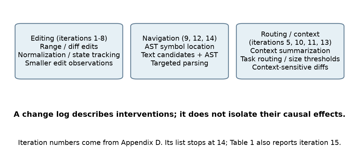
Figure 7. My functional grouping of the changes listed in Appendix D. Groups overlap because one intervention can affect editing, routing, and context. The appendix lists changes through 14, while Table 1 also contains iteration 15; I do not invent a missing fifteenth description.

7.3 Context compression can remove evidence as well as noise

Summarizing relevant code and minimizing diff output can reduce observation size. But an observation is useful precisely because it constrains what the model should believe about the external state. Removing too much context may erase an import, a nearby invariant, an error message, or the reason a previous attempt failed. Compact observations are helpful only when they preserve the information required for the next decision.

This gives a concrete alternative to “always summarize more.” A system could preserve exact locations and changed lines while compressing repetitive context, and request the original material when an uncertainty becomes decision-relevant. The paper’s adaptive program representation makes such policies expressible. It does not measure an information-retention optimum or compare all plausible compression policies.

A change can also be beneficial in one benchmark and harmful in another. Aggressive output minimization may speed synthetic file edits while making a complex repository diagnosis harder. Table 1’s non-monotonic task curves are consistent with such tradeoffs, but they do not uniquely establish this explanation. Runtime noise and unrelated changes can produce similar patterns.

8. Why the reasoning experiment matters

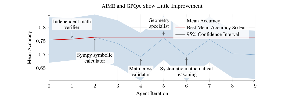
Figure 8. Paper Figure 4, reproduced from v2 p. 7 under CC BY 4.0, by Robeyns, Szummer, and Aitchison. It reports mean accuracy and the best observed mean across AIME 2024 and GPQA Diamond. The confidence band belongs to the original figure; I have not reconstructed it from unavailable raw outcomes.

The second experiment starts from an agent system averaging about 76% across AIME and GPQA Diamond. The paper cites o3-mini-high standalone scores of 87% and 79% on the two benchmarks. Those are contextual model results, not a newly controlled head-to-head experiment in which every inference setting has been matched. The point is that a strong reasoning component is already available, so the surrounding scaffold has less obvious room to help.

The paper describes cases where the main agent largely delegates to the reasoning sub-agent. Added verifiers, symbolic calculators, or specialist roles do not consistently improve the combined outcome. The authors hypothesize that externally imposed reasoning structures may disrupt a reasoning model’s learned process. That is a plausible interpretation of limited gains, but the experiment does not isolate interruption as the unique cause.

There are several alternatives: the chosen changes may be poor; the tasks may offer little benefit from tools; the selection signal may be noisy; the available budget may penalize extra verification; or the initial delegation policy may already be near the useful operating point. Distinguishing these explanations would require ablations and repeated runs. The negative result nonetheless constrains the story: self-editability is not sufficient to guarantee improvement on every domain.

For agent design, I would use the result to ask where the bottleneck lives. If it is file access, tool affordances, or context management, the harness can remove friction. If the model already has a strong internal solution procedure and the task barely touches an external environment, additional coordination may mostly spend time. These are testable categories, not permanent laws separating coding from mathematics.

9. Limitations and failure boundaries

9.1 Repeated optimization on a small fixed task set

The same fixed evaluation population guides repeated selection. Its score is informative about progress on that population, but repeated feedback can favor specialized solutions. An AST locator can be a broadly useful tool and simultaneously exploit the language composition of the development tasks. Those possibilities are compatible. A held-out repository and language evaluation is needed to estimate how far the gain transfers.

A search that repeatedly looks at the same benchmark is also statistically different from testing one predeclared system once. The winner has been chosen using those measurements. Without a separate final evaluation, a selected score can include adaptation to idiosyncratic tasks or favorable noise. The paper provides evidence of an improving development process; it leaves the strength of out-of-distribution generalization less settled.

9.2 Path dependence and proposal quality

The authors explicitly identify difficulty generating novel, feasible, useful ideas. Early ideas can influence later proposals, producing repeated variations of an initially weak direction. Retaining a failure in an archive does not ensure that the next agent will interpret it correctly or explore a genuinely different direction. A detailed archive can become a source of evidence or a source of anchoring.

The expensive part of a bad proposal is not just drafting it. A long editing attempt is followed by another benchmark run. This creates a need to evaluate proposal quality and expected information value, not only downstream task utility. Stronger coding tools may lower implementation cost while leaving the idea-selection bottleneck largely intact.

9.3 Resource constraints define the result

The five-minute timeout can depress the starting score on long-horizon tasks and amplify the value of efficient editing. The authors acknowledge this directly. Removing a bottleneck under a tight budget is still a legitimate contribution. It simply answers a budgeted-performance question, not a budget-independent question about maximum attainable capability.

API prices and latencies are also part of the experiment’s conditions. The paper’s historical dollar figures should not be read as today’s provider pricing. A different model or inference stack can change both the best agent and the utility ranking. The reported token, time, and dollar columns help expose that dependency, but do not eliminate it.

9.4 Observability is incomplete evidence

The paper describes rich traces and an overseer as useful controls. Observability helps people understand failures, but a readable trace is not a guarantee that every important effect is captured. A summary can omit a relevant action; a checker can share an agent’s mistaken assumption; an editable component can change the form of future observations. The paper proposes including additional evaluations before promotion, but does not establish comprehensive behavioral guarantees.

I would keep this limitation proportional to the experiment. SICA demonstrates a bounded, expensive research loop over agent programs. It does not demonstrate an unbounded autonomous system, nor prove that all consequences of arbitrary future edits can be predicted from the supplied traces.

10. Critical analysis: does the better agent become a better inventor?

10.1 Separate useful automation from recursive acceleration

The paper convincingly motivates automated engineering of the agent program. The more ambitious recursive claim concerns the search operator: does selecting a stronger solver make subsequent improvement more effective? These statements are related but logically distinct. Ordinary automated search could find useful agent versions even if the proposal operator remained fixed throughout.

A useful target quantity for that second question is the expected improvement produced by an editor under a fixed search budget. As an analytical definition, let

$$V(g)=\mathbb{E}\left[U_{\mathrm{heldout}}(g')-U_{\mathrm{heldout}}(g) \mid g'\text{ proposed by editor }g,\ \text{fixed budget}\right]. \tag{9}$$

SICA primarily measures the task utility of proposed systems. It does not establish a general monotonic relationship between $U(g)$ and $V(g)$. A faster patch tool plausibly helps both. A policy that over-specializes to a benchmark might improve the first and reduce the second. This is the central uncertainty I would investigate next.

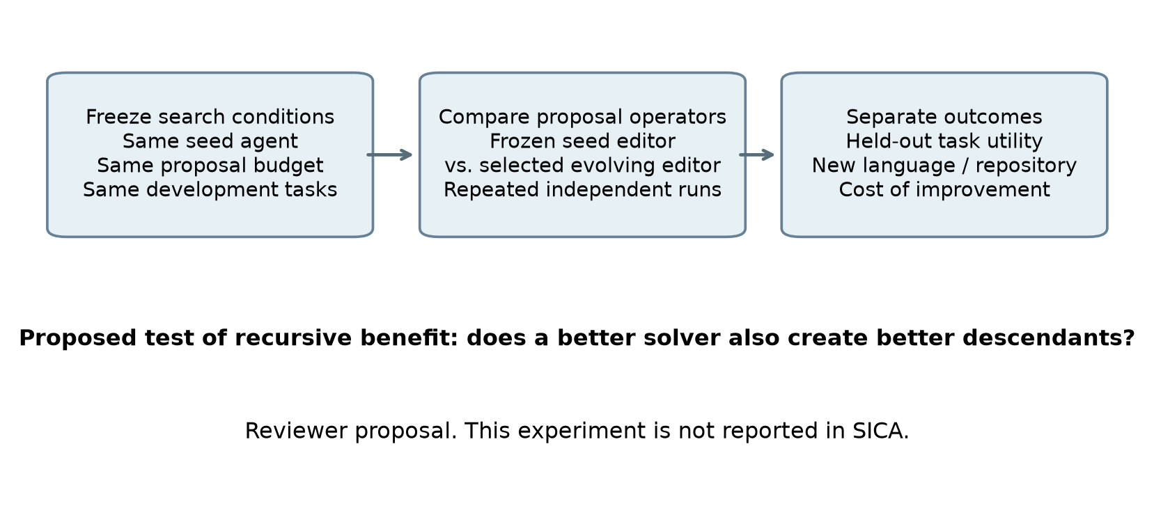
Figure 9. My proposed comparison, not a SICA result. Hold the starting conditions and proposal budget fixed, compare a frozen editor with the evolving selected editor, and judge descendants on held-out tasks as well as search expense.

The clean comparison is not simply “run the system longer.” One arm keeps the initial editing agent fixed while allowing its target programs to change. Another arm lets the selected improved agent become the next editor. Both should receive comparable archive information, evaluation budgets, and task sets. Multiple independent search runs are necessary because path dependence is itself one of the paper’s observed difficulties.

10.2 Measure improvement economics separately

The approximately USD 7,000 search cost and the final per-problem savings answer different questions. Using the rounded Table 1 initial/final costs, the nominal saving is USD 0.21 per problem. If the entire search expense were attributed to obtaining this saving alone, a simplistic break-even volume would be

$$N_{\mathrm{break-even}}=\frac{7000}{1.91-1.70}\approx 33{,}333\text{ problems}. \tag{10}$$

This is a deliberately narrow illustrative calculation, not a deployment forecast. It ignores improved success, human engineering time, infrastructure, changes in task mix, and model pricing. It does show why data efficiency and economic efficiency should not be treated as synonyms. A few improvement iterations can consume a substantial amount of inference compute.

Successful-task cost is another useful metric, but it cannot be honestly recovered here by dividing the all-task mean cost by the SWE-bench score. The numerator and denominator describe different populations. A real estimate would use costs and outcomes for the same task distribution, including retries and failed attempts. Refusing an attractive but mismatched ratio is part of reading the experiment carefully.

10.3 The archive needs structured uncertainty, not only a story

A natural next design is to attach uncertainty and task-level differences to each archived version. Suppose two versions solve different tasks even when their means are similar. That information could motivate conditional routing or a combined tool set. A single scalar rank hides this complementarity. Conversely, two apparently different changes may fail on the same tasks and provide little additional search diversity.

I would retain failure categories, budget exhaustion, affected languages, and a distinction between observed outcomes and explanations. This is a proposal for richer experimental evidence, not a claim that the paper implements such a complete archive. Its existing traces and benchmark summaries are a strong starting point because they make this kind of diagnosis possible.

A held-out score should also be protected from repeated design decisions. Once that score is used to choose the next intervention, it has become development feedback. Calling a set “held out” is insufficient if its results repeatedly steer the search. A final untouched evaluation and independent searches would make the generalization claim easier to assess.

10.4 What I would transfer into a practical harness

The most transferable principle is to make operational bottlenecks visible and editable. Preserve the association between an agent program, its task outcomes, and its resource use. Prefer interventions with a concrete mechanism, such as replacing expensive full-file generation with localized edits. Keep task-solving success separate from the ability to generate useful next changes. Compare against simple routing before adding more roles.

I would not transfer the particular scalar weights unchanged into every product. A research assistant, an interactive coding tool, and an unattended batch fixer have different latency and quality requirements. A hard minimum success condition or a constrained optimization objective may be preferable to trading off every failure against saved time. SICA’s value is that it exposes this choice and makes the surrounding program available for improvement.

11. Conclusion

SICA shows that an agent can improve an editable harness through a loop of archive inspection, code modification, and measured selection, while keeping its foundation models fixed. Its main coding experiment demonstrates substantial gains on the selected SWE-bench tasks, along with uneven improvements across other tasks and resource dimensions. The strongest reading is about reducing friction and improving orchestration under an explicit operating budget.

The remaining question is whether a stronger task solver reliably becomes a stronger improvement operator. That requires more than a rising best-so-far curve. It requires matched search budgets, frozen-versus-evolving editor comparisons, multiple trajectories, and task populations that did not repeatedly steer the design. The paper makes that question concrete enough to study, and its reasoning-task saturation result prevents an overly simple answer.

References and figure provenance

1. Maxime Robeyns, Martin Szummer, Laurence Aitchison. A Self-Improving Coding Agent, arXiv v2, May 16, 2025. Primary source for all reported experimental numbers, Algorithms 1 and utility definitions; full paper and Appendices A-D read.
2. SICA official code resource, linked by the paper.
3. Shengran Hu, Cong Lu, Jeff Clune. Automated Design of Agentic Systems. Related design paradigm discussed in SICA Section 2; no cross-paper numerical ranking is attempted here.
4. Jenny Zhang, Shengran Hu, Cong Lu, Robert Lange, Jeff Clune. Darwin Gödel Machine. Companion reading for archive-based agent evolution; different evaluations and budgets.

Figures 1-3, 7 and 9 are original explanatory diagrams or calculations by Zhongzhu Zhou. Figures 4-6 redraw the rounded values in SICA Table 1. Figure 8 reproduces SICA Figure 4 with attribution under its CC BY 4.0 license. The numerical examples, economic calculation and proposed controlled comparison are my analysis, not additional experiments reported by the paper.