FlashInfer-Bench: Closing the Loop Between Kernel Generation and LLM Serving

Review date: 2026-10-01
Author: Zhongzhu Zhou
Paper reviewed: FlashInfer-Bench: Building the Virtuous Cycle for AI-driven LLM Systems
Paper authors: Shanli Xing, Yiyan Zhai, Alexander Jiang, Yixin Dong, Yong Wu, Zihao Ye, Charlie Ruan, Yingyi Huang, Yineng Zhang, Liangsheng Yin, Aksara Bayyapu, Luis Ceze, Tianqi Chen
arXiv: 2601.00227v1
Version and date: v1, 2026-01-01

1. The contribution I find most useful

A kernel-writing agent can produce a program that compiles, agrees with a reference, and wins a microbenchmark. A serving engineer still needs to know whether that program applies to a particular request, remains valid under the request’s numerical and memory-layout constraints, and improves the complete inference system. FlashInfer-Bench organizes these questions into a common workflow. Its main contribution is the connection between a precise workload description, an evaluation record, and a runtime substitution decision.

I read this as a systems paper about making optimization results usable. The model that generates a kernel is replaceable. The persistent objects are the operator contract, the concrete workload, the proposed solution, and the evidence obtained by evaluating that solution. A well-designed interface between these objects lets many agents contribute without every agent having to redesign the inference engine.

The paper’s snapshot contains eight operator families, 41 definitions, 1,600 workloads, 240 solutions, and 9,600 evaluation records. These are different units. In particular, 9,600 is not the Cartesian product of every solution with every workload: a solution belongs to a compatible definition. The dataset comes from SGLang runs of DeepSeek-V3, Llama-3.1-8B, and Qwen3-30B-A3B using ShareGPT prompts and common serving configurations. The primary agent evaluation uses an NVIDIA B200. These facts describe the January paper, rather than today’s moving leaderboard.

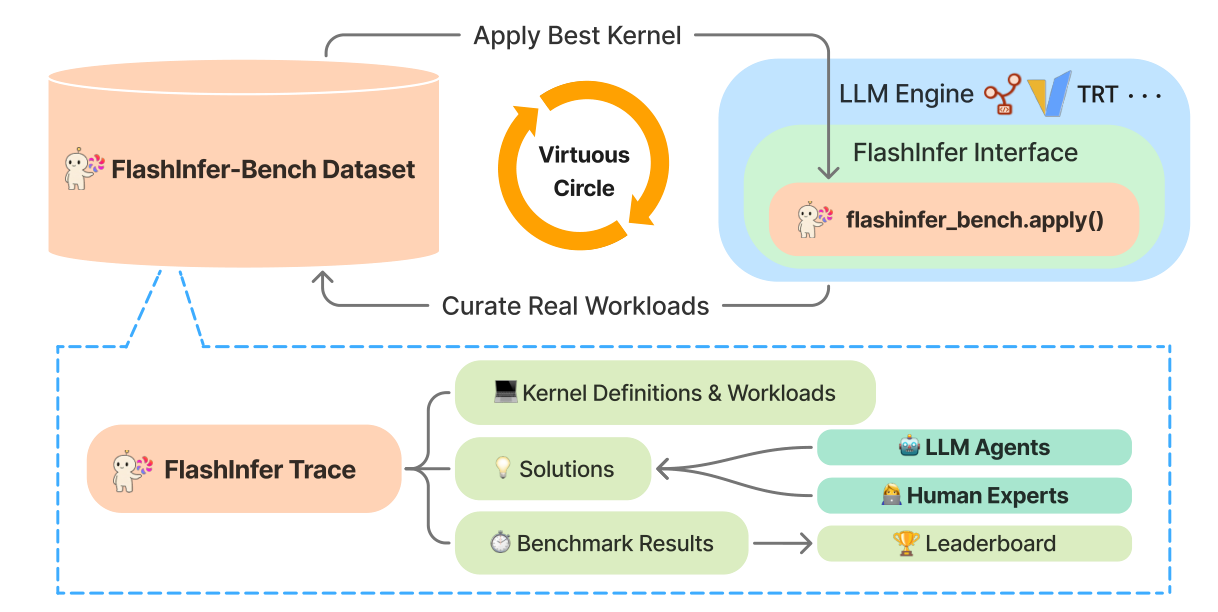
There is an important qualification to the paper’s deployment story. Its Figure 8 demonstrates that substituting different implementations changes end-to-end latency, with small overhead for substituting the original kernel. However, both AI-generated alternatives plotted there are slower than the native FlashInfer baseline. The experiment supports a working integration mechanism and sensitivity to kernel quality; it does not demonstrate an AI-generated end-to-end win over that baseline. I return to the actual numbers in Section 12.

2. Prerequisites: what a kernel result actually means

2.1 Operators, kernels, and complete requests

An operator specifies a mathematical transformation, such as a matrix multiplication. A kernel is a GPU program that implements some or all of that operator. A complete request includes many operator invocations, CPU scheduling, memory management, and often communication. Improving one level does not imply the same proportional improvement at the next level.

For example, a fused add-and-normalization operator can eliminate intermediate memory traffic, but it may occupy only a small fraction of a request’s latency. A tenfold acceleration of that operator does not make the entire request ten times faster. Conversely, adding a few microseconds to a frequently repeated operator can accumulate over layers and generated tokens. This is why a deployable benchmark needs both local timing and a system-level experiment.

2.2 Shape specialization and arithmetic intensity

For a matrix product with $A\in\mathbb R^{M\times K}$ and $B\in\mathbb R^{N\times K}$, the output is $C=AB^\top$. Counting a multiply and an addition as two operations gives approximately $2MNK$ floating-point operations. If ideal traffic includes one read of each input and one write of the output, with $b$ bytes per element, a simple arithmetic-intensity estimate is

$$I=\frac{2MNK}{b(MK+NK+MN)}. \tag{1}$$

This is an explanatory lower-traffic model, not a measurement from the paper. Cache reuse, repeated reads, layout conversions, and intermediate storage change the denominator. It nevertheless explains why the variable dimension $M$ matters even when $N$ and $K$ stay fixed: small matrices may expose launch overhead and insufficient parallelism, whereas large matrices can benefit from more aggressive tiling and tensor-core use.

If peak compute capacity is $P$ operations per second and effective memory bandwidth is $B_w$ bytes per second, the idealized roofline bounds achievable throughput by $\min(P,B_wI)$. Reaching that bound still requires sufficient occupancy and efficient instruction scheduling. A program that implements the right equation with scalar arithmetic can be dramatically slower than one that maps the same equation to tensor cores.

2.3 Ragged batches and paged attention

In decoding, different requests have different context lengths. Padding every request to the longest context wastes work. A paged KV cache instead stores tokens in blocks and uses an index structure to locate each request’s keys and values. Two batches with identical total token counts can have very different length distributions and memory-access behavior.

Grouped-query attention additionally shares KV heads among several query heads. With $H_q$ query heads and $H_{kv}$ KV heads, assuming divisibility and the grouping convention in Appendix A, query head $h$ maps to

$$g(h)=\left\lfloor\frac{h}{H_q/H_{kv}}\right\rfloor. \tag{2}$$

The operator contract must specify this mapping, the page layout, the scaling factor, the output precision, and auxiliary outputs. Matching only the main attention tensor while returning the wrong log-sum-exp output does not satisfy the full contract.

2.4 Correctness references and performance baselines

A clear reference implementation answers what a program should compute. A strong performance baseline answers how quickly an existing system can compute it. They need not be the same program. A Python loop over requests and heads can be an excellent semantic reference and a terrible speed baseline.

The paper says the primary benchmark compares against FlashInfer, using PyTorch when an appropriate FlashInfer implementation is unavailable. Appendix A also contains an illustrative attention trace reporting approximately $1299\times$ relative to its recorded reference latency. That number must not be promoted into a production speedup: its reference and workload context differ from the main benchmark. Keeping the two roles separate is essential to reading this paper accurately.

3. FlashInfer Trace: contracts before optimization

3.1 The four objects

The trace format separates four responsibilities. A Definition describes inputs, outputs, types, dimension axes, constraints, and reference semantics. A Workload binds variable axes and supplies input values. A Solution associates an implementation and compatibility requirements with a definition. An Evaluation ties that specific solution and workload to measured correctness, latency, and an environment snapshot.

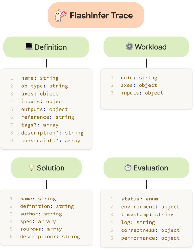
This separation is useful because changing an input shape is different from changing the operator itself. Suppose $N=128$ and $K=2048$ are fixed for a gate projection, while $M$ varies with the number of tokens. The definition fixes the first two dimensions; workloads instantiate $M=6$, $M=64$, and so on. An agent can specialize for known constants without pretending that it supports every matrix shape.

Definitions are deliberately specific. The paper groups invocations only when their interfaces, reference semantics, axis roles, and constant-axis values agree. It discourages optional arguments and behavioral switches: a genuine semantic difference should create a separate definition. The alternative is a large general-purpose interface whose branches may be incompletely exercised. Narrow contracts make dispatch less ambiguous, at the cost of more definitions to maintain.

3.2 A worked attention contract

Appendix A’s example fixes 32 query heads, four KV heads, head dimension 128, and page size one. The variable axes include batch size, number of pages, and the length of the page-index arrays. The pointer array has one more entry than the batch size. For request $b$, its page indices occupy a half-open interval

$$J_b=\mathrm{indices}[\mathrm{indptr}[b]:\mathrm{indptr}[b+1]]. \tag{3}$$

The contract therefore carries both dimensions and input-dependent structure. Supplying random floating-point query tensors is not enough; the integer page mapping must also describe a meaningful request. The example records those structural tensors separately, while other values can be generated at runtime. This is a concrete reason to support both stored inputs and seeded random inputs.

For each head, the reference then computes scaled query-key scores, normalizes them, and combines values. Writing the selected keys and values as $K_{J_b,g(h)}$ and $V_{J_b,g(h)}$, the semantics can be expressed as

$$z_j=\alpha q_{b,h}^{\top}k_{j,g(h)},\qquad o_{b,h}=\frac{\sum_{j\in J_b}e^{z_j}v_{j,g(h)}}{\sum_{j\in J_b}e^{z_j}}. \tag{4}$$

Appendix A also specifies a base-two log-sum-exp. Starting from $Z=\sum_j e^{z_j}$, converting the natural logarithm to base two gives $\log_2 Z=\ln Z/\ln 2$. This conversion is part of the interface, not an optional numerical preference. For empty contexts, the example returns zero attention output and an infinite negative log-sum-exp. That boundary requires explicit treatment when applying the main text’s general rule rejecting non-finite outputs. The paper does not explain this exception in the validation description, so a reader should not assume one universal finite-value rule fits every auxiliary output.

3.3 What the schema does not guarantee

An immutable record preserves what was measured; it does not prove that the recorded workload covers future traffic. A hardware label also does not make performance portable across software versions, clock states, and other loads. The value of a trace is that it makes these dependencies representable and inspectable.

For deployment I would treat the definition and environment as part of the validity domain. A solution that is correct for contiguous BF16 tensors should not silently become the preferred path for a different stride pattern or precision. Some of these conditions can be definition constraints; others belong in compatibility metadata. The paper supplies the framework for making that distinction, but the completeness of each contract remains a substantive engineering question.

4. Curating realistic workloads without erasing the tail

The dataset is extracted from serving runs rather than assembled solely from arbitrary square matrices. This matters for attention, sampling, and MoE. Sequence-length distributions, routing imbalance, and probability distributions can affect cost even when nominal shapes match. The paper records full tensors when values materially affect performance or correctness; otherwise it uses runtime random generation to reduce storage.

It then removes redundant workloads along performance-sensitive dimensions and statistics. Around 50 workloads per definition is the design target, while the concrete snapshot has 1,600 workloads across 41 definitions. The target should not be interpreted as an exact count for every definition.

Algorithm 1. Build a compact workload set

This is my explanatory reconstruction of Section 3.2, not a new measured algorithm. The paper does not specify a complete distance function or a unique rule for representative selection.

1. Run chosen models under stated serving configurations and traffic.
2. Capture operator semantics, fixed axes, variable axes, and inputs.
3. Group calls only when their definition contracts agree.
4. Identify dimensions and values that affect correctness or cost.
5. Store value-sensitive tensors; otherwise store generation metadata.
6. Group redundant cases while preserving important shape diversity.
7. Retain representative workloads for each definition.
8. Freeze the dataset identity used for each reported comparison.

The benefit of reduction is affordable evaluation. A candidate generator may produce many revisions, and testing every real invocation would be expensive. The failure mode is distribution distortion: rare long contexts or highly imbalanced requests may disappear during compression. A benchmark with good operator coverage can still underrepresent the requests responsible for tail latency.

For a simple illustration, batches with lengths $(1,1,1,97)$ and $(25,25,25,25)$ have the same average length and total token count. They can behave differently under a scheduling strategy that assigns one unit of work per request. This example is not a paper experiment; it shows why deduplication based only on an average is insufficient to establish performance equivalence.

An improved evaluation would preserve both representative cases and a separate adversarial or tail set. The former estimates typical behavior; the latter tests the edges of a contract. I would also retain occurrence weights from the serving trace. Equal weighting is appropriate for measuring breadth across cases, but it cannot recover traffic-weighted latency once those weights are discarded.

5. Three different notions of numerical correctness

5.1 Deterministic outputs

For ordinary deterministic operators, the paper compares each output element with a reference. If $a_j$ is the candidate output and $r_j$ the reference, the condition is

$$|a_j-r_j|\leq \epsilon_{\rm abs}+\epsilon_{\rm rel}|r_j|. \tag{5}$$

The absolute term protects values near zero, where relative error becomes unstable. The relative term permits larger absolute deviations when the output magnitude is large. For instance, if both tolerances are $10^{-3}$, the allowed deviation is $0.001$ at zero and $0.101$ at a reference value of 100. These are illustrative tolerances, not values reported for all FlashInfer-Bench tasks.

Every output element must pass for the deterministic rule, and the main text rejects NaN and infinity. Recording maximum absolute and relative errors helps diagnose failures, but those two summaries alone do not show where errors occur. Errors concentrated in a semantically important output can matter more than an equally sized error in an unimportant coordinate.

5.2 Low precision and the matched-ratio rule

Low-bit arithmetic creates larger numerical deviations. Rather than relaxing the bound uniformly, the paper allows a fraction of output elements to miss the tight bound. For an output with $d$ elements, define

$$R=\frac{1}{d}\sum_{j=1}^{d}\mathbf 1\left[|a_j-r_j|\leq\epsilon_{\rm abs}+\epsilon_{\rm rel}|r_j|\right], \qquad R\geq\rho. \tag{6}$$

The paper gives $\rho=0.95$ as an example. This admits a small proportion of outliers without increasing the permitted error everywhere. The trade-off is that the unmatched elements have no magnitude bound in this equation. With 1,000 outputs, 950 perfect values and 50 arbitrarily bad finite values satisfy a 95% matching rule. That arithmetic observation does not mean the reported kernels exhibit such behavior; it identifies what this particular acceptance condition cannot establish.

For a deployment-oriented benchmark, I would report both the matched fraction and a tail-error statistic, such as a high quantile or a norm bound, then relate those errors to model-level quality. A threshold should be justified by the operator’s intended use. It should not be chosen after seeing which value produces an attractive correctness score.

5.3 Sampling: compare distributions, not token equality

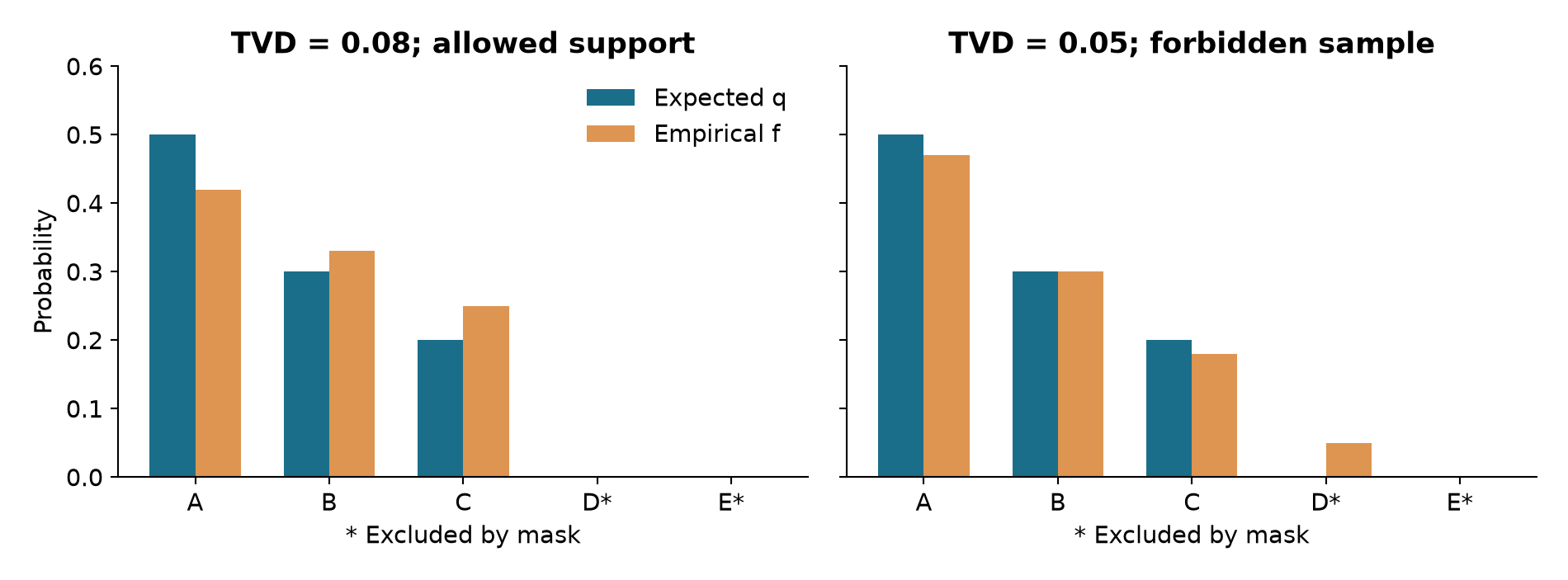
A correct sampler may return a different token on every call. Comparing individual samples with one reference draw is therefore meaningless. The paper forms a target distribution from probabilities $p_j$ and a mask $M_j\in\{0,1\}$, where the mask captures top-k or top-p filtering:

$$Z_M=\sum_j p_jM_j,\qquad q_j=\frac{p_jM_j}{Z_M},\qquad Z_M>0. \tag{7}$$

Repeated candidate calls produce counts $n_j$ from $n$ samples, giving $\hat f_j=n_j/n$. The comparison uses total variation distance:

$$\operatorname{TVD}(\hat f,q)=\frac12\sum_j|\hat f_j-q_j|. \tag{8}$$

To see the meaning of the factor one-half, let $A$ contain coordinates where $\hat f_j>q_j$. The positive excess on $A$ equals the negative deficit outside $A$, because both distributions sum to one. Their absolute differences count that same transferred probability mass twice. Consequently, TVD equals the largest probability discrepancy over any event, $\sup_A|\hat f(A)-q(A)|$.

The paper also requires every sampled token to satisfy the mask. This additional check is necessary: a small TVD can coexist with a forbidden token. In Figure 3, the right example has lower TVD but places positive mass outside the allowed support. It should fail regardless of the global distance threshold.

5.4 Finite samples create uncertainty

Even a perfect sampler produces empirical frequencies different from $q$. A threshold cannot be interpreted without the sample count and the effective support size. Under independent draws from the true target, each frequency has variance $q_j(1-q_j)/n$. Jensen’s inequality and Cauchy-Schwarz give the explanatory bound

$$\begin{aligned} \mathbb E[\operatorname{TVD}(\hat f,q)] &\leq\frac{1}{2\sqrt n}\sum_{j=1}^{K}\sqrt{q_j(1-q_j)}\\ &\leq\frac{1}{2\sqrt n}\sqrt{K\left(1-\sum_jq_j^2\right)} \leq\frac12\sqrt{\frac{K-1}{n}}. \end{aligned} \tag{9}$$

Here $K$ is the size of the target support, not necessarily the whole vocabulary. The last step uses $\sum_jq_j^2\geq1/K$. This is an expectation bound derived for these notes; it is neither a confidence guarantee nor a threshold supplied by the paper. It explains why a single fixed TVD threshold can behave differently for a concentrated distribution and a broad one. The bound is loose when $K$ is large relative to $n$, which is itself a useful warning about relying on empirical TVD alone.

Algorithm 2. Validate according to operator semantics

The following pseudocode summarizes the paper’s three validator branches. Thresholds, trial counts, and handling of legitimate special values must be part of the operator’s declared evaluation policy.

1. Resolve the definition, workload, and numerical acceptance policy.
2. Materialize the required inputs and obtain the reference outputs.
3. Run the candidate and check the complete output structure.
4. For deterministic outputs, require every element to meet its bound.
5. For low-bit outputs, require the declared matched-ratio threshold.
6. For sampling, compute the masked and normalized target distribution.
7. Draw repeated samples; reject any token outside the allowed mask.
8. Compare empirical and target distributions with the TVD threshold.
9. Record errors, acceptance outcome, environment, and trial settings.

The central design choice is to match the test to the semantics. The failure boundary is equally important: passing a finite collection of tests is evidence for those tests, not a proof for every legal input. More trials, carefully selected edge cases, and calibrated stochastic thresholds strengthen the evidence in different ways.

6. Measuring performance without measuring the wrong work

GPU execution is asynchronous with respect to the CPU. A host timer around a launch may mostly measure submission latency. The paper instead uses CUDA events for device-side timing, performs $w$ warmup runs, and reports the mean of $m$ measured runs. A per-device lock coordinates cooperating benchmark processes so two timed jobs do not compete on the same GPU.

The distinction between cooperating processes and the entire machine matters. A lock within the benchmark does not establish that every unrelated workload, device clock change, or thermal event is controlled. The evaluation environment should record the relevant conditions. Warmup also changes the question: the reported latency estimates a prepared steady state, while first-use compilation and initialization are separate costs.

FlashInfer-Bench provides persistent workers and fully isolated subprocess runs. Persistent workers amortize initialization and preserve useful caches. Isolated runs tear down the CUDA context after completion or timeout, reducing cross-solution state carryover. These are practical choices for evaluating many expensive candidates; they have different costs and different isolation properties.

The described default is persistent execution, with repeatedly failing solutions deferred to isolated runs. This detail limits how strongly one can summarize the framework as universally isolated. A deployment claim should state which measurements came from which mode. Process separation is also not equivalent to complete protection against arbitrary host behavior; the paper’s scope is a benchmarking mechanism, and stronger security conclusions need separate evidence.

6.1 Scheduling evaluations across devices

The benchmark service builds a cost matrix for ready solution-workload jobs and device workers, accounting for warm compilation caches and baseline residency. It assigns small batches using the Hungarian algorithm and updates cost estimates online. The idea is to schedule related work near useful cached state without allowing simultaneous timing interference.

A conventional exponentially weighted estimate has the form

$$\hat c_{t+1}=\beta\hat c_t+(1-\beta)c_t,\qquad 0\leq\beta<1. \tag{10}$$

This equation explains the moving-average idea mentioned by the paper; no particular $\beta$ is reported here. Large $\beta$ smooths noise but adapts slowly when a new class of workloads arrives. Small $\beta$ adapts quickly but reacts strongly to unusual measurements. The assignment policy optimizes evaluation throughput, whereas the final kernel timing estimates serving performance. Those are separate objectives even though both are measured in time.

7. The agent loop: feedback is only as good as its objective

The paper evaluates a straightforward feedback-loop agent. It receives an operator definition, a target language, and hardware information, proposes a solution, receives benchmark feedback, and revises the proposal. The best passing candidate is retained. This arrangement avoids conflating the framework contribution with a particularly elaborate agent architecture.

Algorithm 3. Generate, measure, revise, retain

This restates paper Algorithm 1 with an explicit no-success case. The aggregate score used to select the best candidate must be specified when several workloads are involved.

1. Initialize the agent with definition, language, and target hardware.
2. Generate the initial candidate and initialize an empty valid set.
3. For each iteration within the stated budget:
4.     Evaluate the candidate against the designated workloads.
5.     If it passes, store the candidate and its evaluation record.
6.     Provide errors and performance measurements to the agent.
7.     Ask for a revised candidate without changing the task contract.
8. If no candidate passed, return failure and retain the fallback.
9. Otherwise select the valid candidate with the best declared score.

The distinction between correctness repair and speed optimization appears in Appendix C’s prompts. A model with a compilation error is first asked to repair it; a correct model is asked to improve memory access, launch geometry, and related choices. Feedback can make this process more effective than one-shot generation, but it also encourages overfitting to whichever examples are repeatedly visible.

I would separate tuning workloads from final evaluation workloads at the level of meaningful shapes and distributions, rather than merely changing random seeds. Otherwise an agent can learn a dispatcher that performs well on familiar shapes while offering little generalization. The paper mentions hidden workloads in the leaderboard design, but it does not provide a complete split and search-budget accounting for every result in the static paper.

There is another design choice: allowing library calls. The authors observe that some CUDA solutions use cuBLAS rather than developing a new low-level kernel. This can be excellent engineering and weak evidence of novel kernel synthesis at the same time. A benchmark should declare whether it measures unrestricted operator implementation, new kernel construction, or knowledge of existing libraries. None of these is intrinsically the wrong task; mixing them under one interpretation is the problem.

8. Reading fast-p curves carefully

Let $c_i$ indicate whether workload $i$ passes validation, and let $s_i=t_i^{\rm base}/t_i^{\rm cand}$ be its speedup. The paper adopts the KernelBench metric

$$\operatorname{fast}_p=\frac1N\sum_{i=1}^N c_i\mathbf1[s_i>p]. \tag{11}$$

For positive execution times, $p=0$ measures the fraction correct. At $p=1$, it measures the fraction both correct and strictly faster than the baseline. At $p=0.95$, a correct candidate can be slightly slower and still count. Specifically, $s>0.95$ permits candidate latency below $t^{\rm base}/0.95$, approximately 5.26% above baseline latency. Ranking at 0.95 is therefore a near-parity criterion, not a strict improvement criterion.

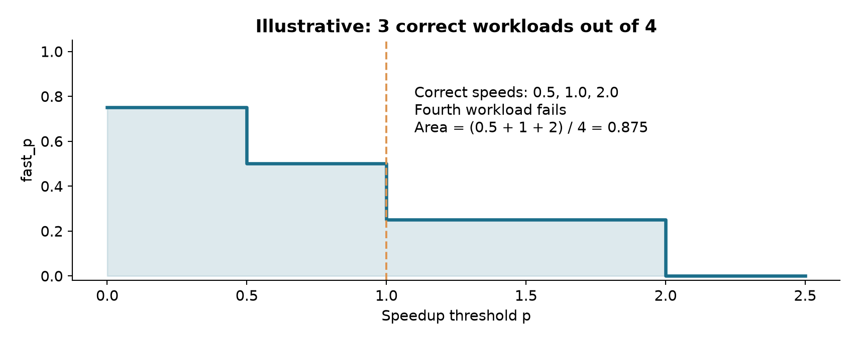
The curve is a correctness-weighted survival function of speedup. Its area has a precise interpretation. Since the area under $\mathbf1[s_i>p]$ from zero to infinity is $s_i$,

$$\int_0^\infty\operatorname{fast}_p\,dp =\frac1N\sum_i c_is_i. \tag{12}$$

For an axis truncated at $P$, the contribution becomes $c_i\min(s_i,P)$. This derivation assumes a linear threshold axis and the same workload weighting. An area on a logarithmic axis would have a different interpretation. The paper describes AUC as an overall measure; it should be accompanied by the actual integration range and aggregation policy.

In Figure 4, correct speedups are 0.5, 1, and 2, while a fourth workload fails. The full area is $(0.5+1+2)/4=0.875$, the correctness rate is 0.75, and $\operatorname{fast}_1=0.25$. An incorrect candidate with an apparently enormous speedup contributes zero. This is a useful safeguard, but it still depends on the validator actually detecting incorrect behavior.

8.1 Equal workload weight is not equal serving importance

An arithmetic mean of speedup ratios can be dominated by a large improvement on a tiny operation. A traffic-weighted latency comparison instead considers how often each operation occurs and how much time it occupies. Under a simple serial model with occurrence weights $w_i$, the aggregate speedup is

$$S_{\rm weighted}=\frac{\sum_iw_it_i^{\rm base}}{\sum_iw_it_i^{\rm cand}}. \tag{13}$$

Consider a 1-microsecond operation improved to 0.1 microseconds and a 100-microsecond operation worsened to 125 microseconds, each occurring once. The arithmetic mean of local ratios is $(10+0.8)/2=5.4$, yet total time increases from 101 to 125.1 microseconds. The ratio of totals is about 0.807. These illustrative numbers explain why fast-p curves should accompany, rather than replace, an end-to-end measurement.

9. Applying a result to a serving engine

The apply() mechanism turns evaluated candidates into operator replacements. A decorator associates a serving function with a fixed definition or a resolver that derives the definition from runtime arguments. The original function supplies a fallback. An imperative API provides a direct invocation path. Integration with FlashInfer enables compatible operators to be redirected without changing each serving engine call site.

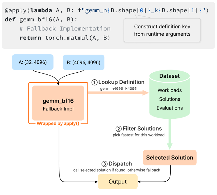
Most selection work is performed before serving starts. The system filters evaluation records according to acceptance requirements, creates workload feature keys, chooses the fastest accepted candidate for each key, and compiles frequently selected candidates ahead of time. Less frequent choices can be compiled on demand. Online dispatch then uses a small number of index lookups.

Algorithm 4. Build and use a dispatch index

This is an explanatory expansion of Section 3.5. The contract and compatibility guards are necessary to interpret the selected entry; the pseudocode is not an implementation prescription.

1. Load the chosen dataset and evaluation snapshot.
2. Discard candidates that fail the declared numerical requirements.
3. Filter by compatible definition and execution environment.
4. Construct a feature key for each supported workload.
5. Associate each key with the lowest-latency accepted candidate.
6. Compile frequent choices ahead of time; prepare remaining choices.
7. On a serving call, resolve its definition and workload key.
8. If a valid matching choice exists, invoke it.
9. Otherwise invoke the original fallback function.

The attraction is clear: expensive evaluation produces a reusable dispatch table rather than a report that an engineer must translate manually into engine modifications. It is also easy to disable substitution globally and recover the original behavior. This fallback is useful when a new shape has no validated candidate.

9.1 The information lost when a trace becomes a key

An evaluation record can contain actual tensor values, but a fast runtime key commonly includes shapes and a limited feature set. That is a compression of information. If two workloads share a key while differing in an input-dependent performance characteristic, choosing the faster candidate for one does not establish optimality for the other.

For example, the paper itself notes that sampling cost can depend on the probability distribution. Identical batch and vocabulary sizes do not imply the same effective top-p support. A shape-only dispatcher can remain mathematically correct yet choose a poor performance path. It should either incorporate the relevant inexpensive statistic, select a robust candidate, or keep the native fallback when evidence is insufficient.

There is also a first-use question. Constant-time lookup does not imply constant-time compilation. Ahead-of-time preparation and CUDA graph warmup can make steady-state overhead small, while an unseen key that triggers compilation can cause a latency spike. Both paths belong in a deployment evaluation; reporting only the prepared path answers only one of the two questions.

10. What the model comparison actually establishes

The static evaluation uses frontier models available in the paper’s study: GPT-5, o3, Gemini 2.5 Pro, and Claude Opus 4.1. Results should be read as that snapshot, not as a current model ranking. Figure 7’s language comparison reports the following correctness percentages:

Model	CUDA	Triton
GPT-5	83	96
o3	58	96
Gemini 2.5 Pro	29	79
Claude Opus 4.1	25	83

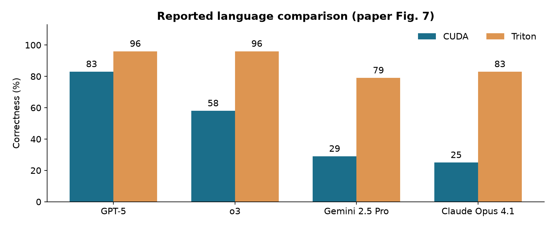
This supports a language-abstraction effect under the tested generation procedure. It does not establish that Triton is always faster, nor that the models have the same intrinsic ability independent of their compiler. A high-level language delegates important decisions to a compiler; that delegation is part of the system being evaluated.

The authors report that 30 of 32 observed correctness errors were compilation failures. The remaining two involved runtime or numerical errors. That is a concrete failure breakdown for the analyzed set, not a universal statement that numerical mistakes are rare in generated kernels. A candidate that cannot compile never reaches many numerical tests, so the visible failure distribution depends on the order of the checks and the maturity of the generator.

The main examples include API misuse, host/device confusion, and type or shape mistakes. These suggest a practical improvement direction: provide accurate interface constraints and feedback before investing the entire search budget in sophisticated optimization prompts. However, fixing compilation is only the entry ticket. Correct scalar code may still be far below a tuned library.

Figure 4’s leaderboard screenshot and Figure 7’s language split also should not be casually combined. They show different summaries, and the paper does not give enough aggregation detail to derive every displayed percentage from the other. I retain each figure’s stated scope instead of averaging them into a new headline number.

11. The GEMM and attention case studies

11.1 Why the compiler can dominate the comparison

Section 4.4 reports mean GEMM times of 0.11 ms for a generated Triton kernel and 0.5 ms for a generated CUDA kernel, a ratio of roughly $4.5\times$. The explanation emphasizes compiler-provided pipelining, tile selection, and use of newer tensor-core instructions. The CUDA discussion describes a load-synchronize-compute-synchronize structure with WMMA, while the Triton discussion describes four autotuning configurations and compiler support for Blackwell’s tcgen05 instructions.

The relevant intuition is coordination cost. Efficient kernels require choices about data movement, synchronization, shared memory, registers, and matrix instructions to work together. A generator that expresses a tile-level operation in a DSL can rely on the compiler for some of that coordination. A generator writing lower-level CUDA must get more interacting details right itself.

This is evidence for evaluating the model-language-compiler combination. It is not a controlled experiment isolating only language syntax: the search space, automatic tuning, compiler transformations, and possibly generated solution identity all change. A fair follow-up would keep the model, definition, candidate budget, and hardware fixed while separately enabling each source of automatic optimization.

11.2 The appendix needs a careful reading

Appendix B provides selected example summaries. Their listed speedups relative to their stated baselines are:

Appendix example	Listed across-workload speedup	Listed best case
B.1 GPT-5 Triton GEMM	0.20×	0.60×
B.2 Gemini CUDA GEMM using cuBLAS	0.97×	1.03×
B.3 o3 Triton GQA decode	0.19×	0.98×
B.4 GPT-5 CUDA GQA decode	0.02×	1.02×

A speedup below one is a slowdown. Thus a large improvement over another generated kernel can coexist with poor performance against the production baseline. The $4.5\times$ number from the main text and the 0.20× result in Appendix B.1 answer different comparison questions.

There is a further presentation inconsistency: Section 4.4 points to B.1 and B.2 as the implementations for its GPT-5 Triton/CUDA comparison, but B.2 labels its example as Gemini 2.5 Pro calling cuBLAS. I do not equate those examples or infer a corrected experiment. The safe conclusion is that the narrative and appendix are not sufficient to reconstruct the exact paired comparison from those references alone.

11.3 Online softmax is necessary but not sufficient

For attention, implementing online softmax removes the need to materialize every attention probability. Suppose the current processed block has maximum $m$, exponential sum $l$, and weighted-value accumulator $o$. A new block has $m'$, $l'$, and $o'$. To combine both while preserving a common exponent scale, set $M=\max(m,m')$ and rescale:

$$\begin{aligned} l_{\rm new}&=e^{m-M}l+e^{m'-M}l',\\ o_{\rm new}&=e^{m-M}o+e^{m'-M}o',\\ y&=o_{\rm new}/l_{\rm new}. \end{aligned} \tag{14}$$

This identity follows by multiplying numerator and denominator contributions by the same common factor $e^{-M}$. It explains how intermediate state stays bounded without changing the attention result in exact arithmetic. It does not automatically supply efficient GPU tiling, asynchronous loads, tensor-core mapping, or enough parallelism.

The paper reports that explicitly prompting GPT-5 with more advanced attention optimization advice still failed to produce a correct implementation of those optimizations in ten attempts. That is a useful local observation, with a small and specific attempt budget. It should not become a claim that all agents cannot perform the task. The broad lesson is that stating an optimization in words and coordinating its low-level realization are different capabilities.

12. End-to-end evidence: recalculate before repeating the claim

The substitution experiment uses fused add RMSNorm with hidden size 4096 inside SGLang serving Llama-3.1-8B-Instruct. The three batch/concurrency settings are 1, 16, and 64. The paper says it warms up the system and measures mean latency over four requests with the same input and output lengths. That is a small controlled demonstration, not a production traffic study.

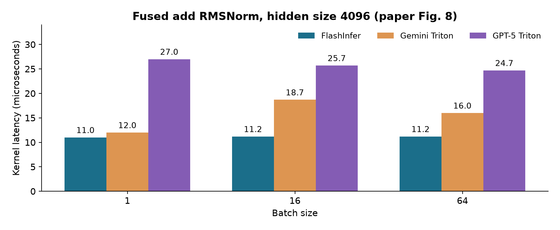
At batch 64, FlashInfer takes 11.2 microseconds, Gemini’s generated Triton alternative takes 16.0, and GPT-5’s takes 24.7. Relative to FlashInfer, their speedups are $11.2/16.0=0.70$ and $11.2/24.7\approx0.453$. These calculations make the ordering unambiguous. The text that introduces Gemini as faster than baseline conflicts with the plotted values.

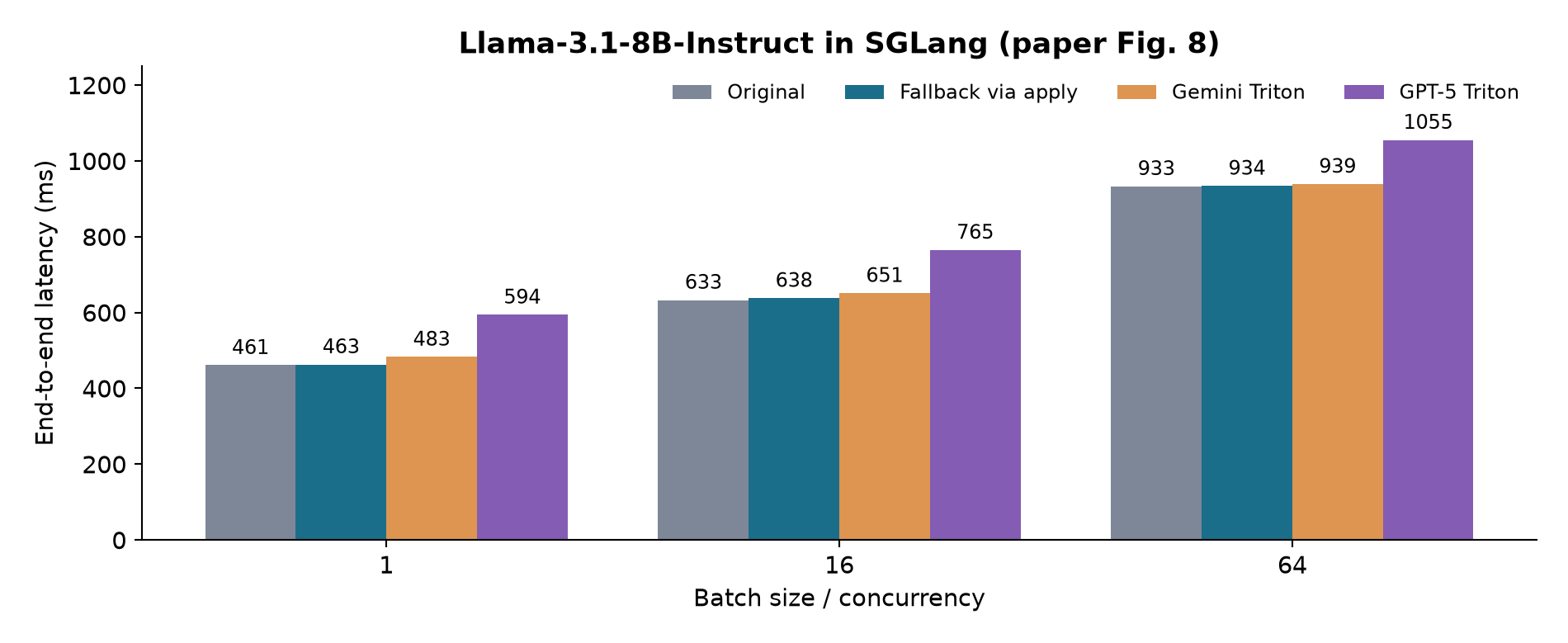
The original-to-fallback pairs are 461/463, 633/638, and 933/934 ms. The calculated overheads are approximately 0.434%, 0.790%, and 0.107%. These agree with the paper’s statement that the end-to-end overhead is below 0.8%. The reported per-invocation dispatch overhead is 1–2 microseconds; it should be distinguished from these whole-request percentages.

At batch 64, fallback substitution, Gemini, and GPT-5 take 934, 939, and 1055 ms. The ordering tracks local kernel quality, but neither generated kernel improves the native 933 ms result. Gemini reduces latency relative to the slower generated GPT-5 kernel, not relative to FlashInfer. At batch 1 the same distinction is stronger: the native result is 461 ms, compared with 483 and 594 ms for the two generated alternatives.

This does not undermine the usefulness of substitution. A benchmark needs a mechanism that faithfully carries both improvements and regressions into the complete system. It does limit the empirical conclusion: the plotted example demonstrates low replacement overhead and a relationship between kernel quality and request latency. The paper would need a candidate faster than the native kernel, with a robust whole-system comparison, to demonstrate the stronger improvement claim.

12.1 Amdahl’s law with dispatch cost

Let $T$ be the original request latency, let fraction $f$ be spent in the operator being replaced, and let $s$ be its local speedup. If the remaining work does not change and the extra dispatch cost is $\delta T$, then

$$T_{\rm new}=T(1-f)+\frac{Tf}{s}+\delta T, \qquad S_{\rm end}=\frac{1}{(1-f)+f/s+\delta}. \tag{15}$$

This is an explanatory model, not a fitted estimate for Figure 8. It assumes the affected work lies on the relevant serial critical path; overlap, changed scheduling, and memory contention can break the decomposition. Setting $f=0.1$, $s=2$, and $\delta=0.01$ gives an end-to-end speedup of $1/0.96\approx1.042$. A twofold local improvement then yields only about 4.2% overall.

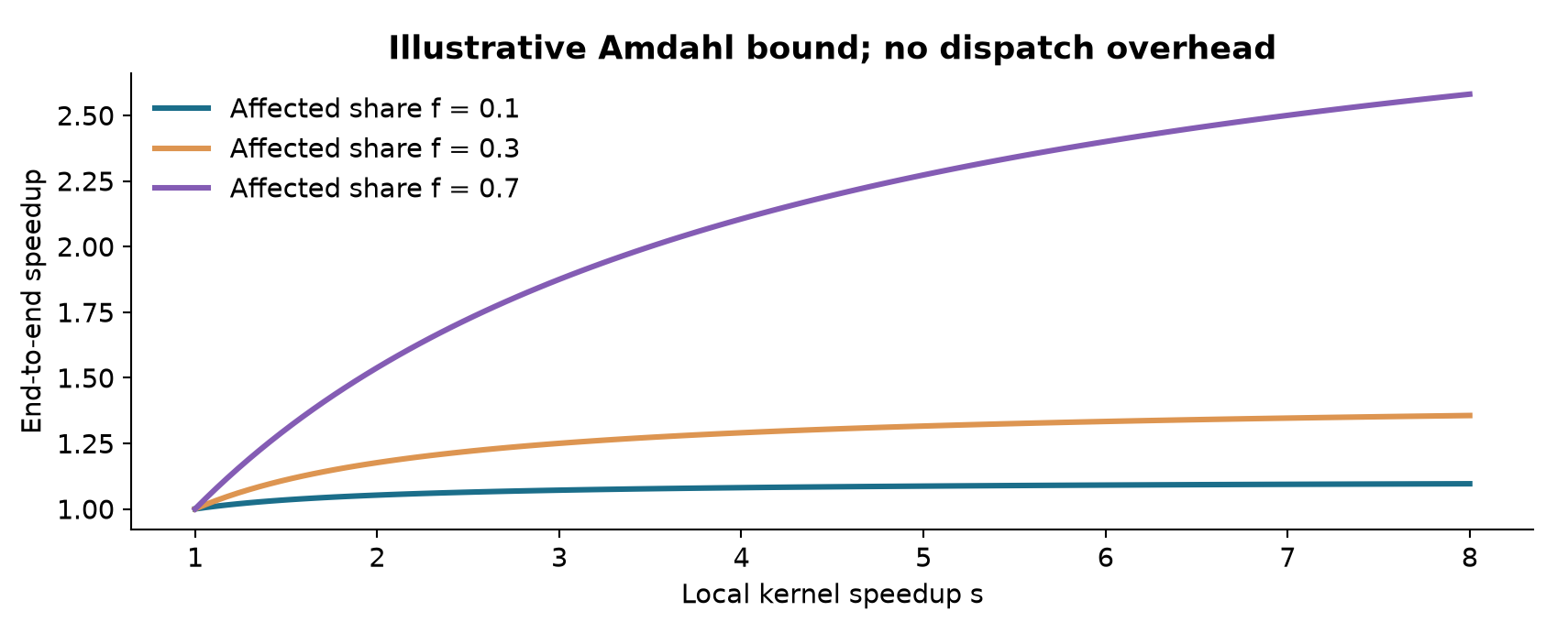
Rearranging Equation 15 yields a useful deployment condition: substitution is beneficial only when $f(1-1/s)>\delta$. The saved time must exceed the added overhead. This condition also explains why a dispatcher should retain the native implementation among its performance choices. Choosing the fastest generated candidate is insufficient if all generated candidates are slower than the native path.

12.2 Why four requests are not an uncertainty analysis

The figure reports means without variation estimates. When the observed fallback difference is 1–5 ms, one needs run-to-run variability to judge the precision of that difference. Repeated paired measurements, randomized execution order, and confidence intervals would make the comparison more persuasive. Tail percentiles and throughput under a stated arrival process would answer additional serving questions that a mean over four requests cannot.

The relationship between isolated kernel timing and end-to-end timing is also not expected to be linear across all batch sizes. The number of invocations, critical-path overlap, graph capture, and scheduling can change. The paper’s three points show a qualitative ordering. They do not identify a universal conversion factor from microseconds saved in one kernel to milliseconds saved in a request.

13. What a stronger follow-up evaluation should report

I have not run the paper’s GPU experiments. The numerical work in these notes consists of explicit recalculation of published values and labeled explanatory examples. The following is a study design for evaluating the paper’s claims, rather than a report of completed experiments.

First, freeze the task population: definition identities, workload values or seeds, numerical policies, hardware, software environment, and baseline identities. Keep semantic references and performance baselines as separate fields in the report. Record both the initial and final candidate-selection rules so the reported result can be tied to a specific search process.

Second, report search cost as a budget vector. Number of iterations alone is not enough when models consume different token counts, compiler time, autotuning time, or GPU evaluation time. For each model-language pair, record attempts, successful candidates, total wall time, and the cost of producing the final result. A DSL with a larger automatic search budget may deserve the performance credit, but that budget should be visible.

Third, use separate development, held-out, and stress workloads. Development inputs support feedback. Held-out workloads estimate transfer. Stress cases target numerical extremes, unusual ragged distributions, and boundary shapes. The split should preserve the relevant contracts while making it difficult to succeed solely by memorizing a small dispatch table.

Fourth, evaluate deployment in stages. Compare the native path with an identical fallback passed through substitution to estimate overhead. Compare validated generated candidates with the same native baseline. Report warm and cold behavior separately, then run a controlled traffic mix with latency percentiles and throughput. For stochastic kernels, state sample counts and acceptance thresholds; for low-bit kernels, include error tails and model-level quality.

Finally, distinguish the benchmark’s frozen snapshot from a rolling leaderboard. A continuously improving dataset is valuable for engineering, while a reproducible scientific comparison needs stable task identities and definitions. Both can coexist if each published result identifies which population and environment it refers to.

14. Limitations and failure boundaries

The authors explicitly note limited coverage of models, hardware, and programming languages, and the absence of multi-GPU communication kernels. A service that schedules independent evaluations across several GPUs is not the same as evaluating one distributed kernel spanning several GPUs. Extending to collectives introduces ordering, communication-computation overlap, and failure behavior beyond the present single-kernel model.

The serving traces are more relevant than arbitrary operator shapes, but they remain a sample from selected models, configurations, and traffic. Changes in quantization, context length, batching policy, or MoE routing can change both the dominant kernels and the best implementations. A fixed dispatch table therefore has a validity period and domain, rather than universal applicability.

Numerical acceptance is finite and policy-dependent. Elementwise tolerances, a matched ratio, and empirical TVD address different failure modes, but none alone proves equivalence for all inputs or preservation of complete-model quality. The special-value behavior in the attention example illustrates why validation must be attached to the exact contract.

The low end-to-end overhead result is strongest for prepared execution. It does not fully characterize just-in-time compilation, cache misses, or workload drift. The experimental example also covers one normalization operator inside one model and engine configuration. Broader engine integration is a framework capability, not equivalent to broad end-to-end empirical validation.

15. Critical analysis: where the argument can be made stronger

15.1 Keep three claims separate

The paper bundles an expressive task format, a usable substitution mechanism, and a promise of continuously improving serving performance. The first two are supported by concrete design and an integration experiment. The third requires stronger evidence than the particular Figure 8 example provides. Treating these claims separately makes the work more useful: its infrastructure contribution does not need an exaggerated acceleration headline.

A decisive follow-up would retain the native kernel as a candidate, present a generated replacement that wins held-out local tests, and demonstrate the improvement under repeated whole-system measurements. If no such candidate wins, a successful dispatcher should select the native path. The ability to decline a bad optimization is itself a meaningful systems property.

15.2 The schema should preserve uncertainty, not only results

An evaluation object is described as immutable, which is valuable for provenance. Yet a single latency and a pass/fail outcome hide uncertainty. For selection among many candidates, the minimum observed latency can be optimistically biased simply because many noisy estimates were compared. The more candidates an agent tries, the more opportunities it has to select a lucky measurement.

I would attach sample counts, spread estimates, and independent confirmation measurements to selected candidates. For close races, the policy could require an improvement margin exceeding measurement uncertainty. This changes the question from which candidate has the smallest observed number to which candidate has enough evidence to justify replacement.

15.3 Numerical policies can become optimization targets

The matched-ratio rule intentionally ignores a small fraction of errors. Repeated optimization against that rule can reward concentrating error into the allowed fraction, even without malicious intent. Similarly, a stochastic test with insufficient samples can miss rare but meaningful probability distortion. These are properties of the objective, not accusations about the authors’ reported candidates.

The remedy is to make failure costs visible at multiple levels: support validity, distribution distance with calibrated sampling uncertainty, error magnitude tails, and downstream model quality. A benchmark should keep those components separately reportable rather than collapse every notion of correctness into a single unexplained Boolean.

15.4 Real workload collection needs an explicit generalization test

Collecting production-like traces improves relevance, but repeatedly tuning on a finite trace set can turn realism into memorization. The solution is not merely collecting more cases. One needs a split that reflects the anticipated deployment change: unseen sequence-length distributions, another batching regime, a related model, or a changed precision mode.

The paper’s specific definitions make such tests easier to describe. I would use that structure to separate within-definition interpolation from transfer to a new definition. An agent may excel at choosing tile parameters for known shapes while struggling to adapt to a different data layout. Those are different capabilities and should produce different claims.

15.5 Abstraction deserves credit, and cost accounting

The Triton result suggests that a strong compiler is an effective partner for a code-generating model. It does not require framing low-level generation as the only legitimate form of intelligence. Production systems often benefit from combining generated glue, existing libraries, and specialized kernels.

At the same time, evaluations of new kernel synthesis should distinguish library reuse from new algorithms. Reporting both unrestricted engineering performance and restricted synthesis performance would preserve practical relevance while making the capability claim sharper. Matching search budgets would further reveal whether gains come from language abstraction, automated tuning, or model reasoning.

16. Conclusion

FlashInfer-Bench offers a useful way to turn kernel experiments into structured, reusable serving decisions. The most durable ideas are specific operator contracts, workload-aware evaluation, separate validation policies for different numerical semantics, and a fallback-capable substitution path. Together they reduce the engineering distance between a generated candidate and an inference engine.

The paper also illustrates how demanding it is to substantiate a systems improvement. Correctness rates, local speedups, and whole-request latency answer different questions. A comparison with another generated kernel is different from a comparison with a tuned production baseline. The end-to-end figure establishes a working replacement mechanism and small overhead, while leaving a stronger native-baseline acceleration claim unproven in that example.

My practical takeaway is to preserve the full chain of evidence: precise contract, representative workload, calibrated validation, strong baseline, cost-aware selection, and whole-system measurement. A closed optimization loop becomes valuable when every link carries the conditions under which its result remains true.

References and reading pointers

1. Shanli Xing et al. FlashInfer-Bench: Building the Virtuous Cycle for AI-driven LLM Systems, v1, 2026-01-01. Primary source for all reported experiments and the three cropped figures; Sections 3–4 and Appendices A–C were read in the complete 39-page paper.
2. FlashInfer-Bench project. Resource entry; the analysis above uses the fixed paper snapshot rather than a current leaderboard ranking.
3. Anne Ouyang et al. KernelBench: Can LLMs Write Efficient GPU Kernels?. Background source for the fast-p metric adopted by FlashInfer-Bench.
4. Zihao Ye et al. FlashInfer: Efficient and Customizable Attention Engine for LLM Inference Serving. Background on the kernel library used as the principal performance baseline.

Equations 1–4, 9–10, and 12–15 supply explanatory modeling or derivations around the paper’s method. Equations 5–8 and 11 express its stated acceptance rules and metric. Figures 3, 4, and 9 are illustrative calculations; Figures 6–8 redraw reported data. No new GPU performance measurements are claimed.