Fast-dLLM: Reusing Bidirectional State and Spending Confidence on Parallel Tokens

Review date: 2026-09-30
Author: Zhongzhu Zhou
Paper: Fast-dLLM: Training-free Acceleration of Diffusion LLM by Enabling KV Cache and Parallel Decoding
Paper authors: Chengyue Wu, Hao Zhang, Shuchen Xue, Zhijian Liu, Shizhe Diao, Ligeng Zhu, Ping Luo, Song Han, Enze Xie
Version: arXiv:2505.22618v3, 3 July 2025; first submitted 28 May 2025
Resources: Paper PDF, author project page, official repository.

1. The useful question behind the headline

A masked diffusion language model can predict many missing tokens in one forward pass. That sounds like a direct route to fast generation, but two obstacles intervene. First, the model repeatedly processes positions whose visible tokens have barely changed. Second, filling many blanks from separate marginal predictions can produce a combination that the model would not prefer jointly. More parallel prediction is therefore not automatically more useful completed text per second.

Fast-dLLM addresses both obstacles without retraining the base diffusion model. It reuses key and value states over short intervals, then refreshes them. It also selects how many tokens to commit from the current confidence estimates, rather than forcing a fixed number at every step. The experimental contribution is substantial: these two changes accelerate LLaDA and Dream across mathematical and coding tasks. The paper also supplies an informative worst-case theorem about when marginally confident choices agree with the joint most probable choice.

My reading is that the method spends two kinds of approximation budget: one on stale representations, and one on token dependence. These budgets interact. A confidence value computed with approximate cached states is not automatically the confidence assumed by a theorem about a coherent joint distribution. That distinction is central to understanding both the design and its limits.

The much-quoted 27.6-fold throughput improvement is a specific LLaDA configuration: eight-shot GSM8K, generation length 1,024, and DualCache with parallel decoding. The reported throughput moves from 0.7 to 19.3 tokens per second; accuracy moves from 77.3 to 76.0. Those absolute numbers, the workload, and the quality difference belong beside the ratio. The result is neither a universal diffusion-model speedup nor a comparison against a highly optimized autoregressive serving system.

This review separates reported measurements, algebraic consequences, and my proposed follow-up experiments. The figures redraw reported values where indicated; the probability examples and cost model are explanatory calculations, not new model measurements.

2. Prerequisites: what the model predicts and what a cache stores

Let a prompt have length P and a requested answer have length L. A masked diffusion model starts with the answer positions masked and repeatedly predicts missing tokens while conditioning on the prompt and already visible answer tokens. Unlike causal decoding, a visible position may attend to positions on both sides. The relevant context is therefore the entire partly completed sequence, not just its left prefix.

For a clean token sequence x_0, a simple forward masking process independently replaces each token with a mask with probability t:

$$q_t(x_t\mid x_0)=\prod_i\left[(1-t)\mathbf 1\{x_t^i=x_0^i\}+t\mathbf 1\{x_t^i=\mathrm{MASK}\}\right]. \tag{1}$$

Here t=0 is clean text and t=1 is fully masked text. During learning, predictions at masked positions teach the denoiser to recover the original tokens. During generation, a decoder decides which predictions to commit and how much of the answer to expose at each iteration. The model architecture and the decoding policy are distinct: a model capable of simultaneous prediction can still be decoded conservatively, one position at a time.

For reverse times s<t, the standard absorbing-mask transition preserves an already visible token. At a still-masked position, it retains the mask with probability s/t and otherwise samples a token from the denoiser:

$$p_\theta(x_s^i\mid x_t)= \begin{cases} \delta_{x_t^i}, & x_t^i\ne\mathrm{MASK},\\ \frac{s}{t}\delta_{\mathrm{MASK}}+\left(1-\frac{s}{t}\right)p_\theta(x_0^i\mid x_t), & x_t^i=\mathrm{MASK}. \end{cases} \tag{2}$$

Fast-dLLM’s confidence-aware policy changes the schedule of commitments. Its practical decoding should not be interpreted as sampling exactly from every transition of an unchanged diffusion chain. Once a selected token is unmasked, the described algorithm does not revise it later. Early mistakes can therefore change the context used for subsequent decisions.

At an attention layer, queries Q compare with keys K, and the resulting weights combine values V:

$$\operatorname{Attn}(Q,K,V)=\operatorname{softmax}\left(\frac{QK^\top}{\sqrt d}\right)V. \tag{3}$$

A KV cache stores K and V so they need not be regenerated for selected positions on every forward pass. It does not make their attention contribution disappear. An active query can still attend to a cached prefix, and the corresponding scores and value aggregation still require work. This matters when translating a smaller recomputed token region into an actual runtime estimate.

Autoregressive caching has an unusually strong justification: under causal attention, appending a future token cannot change an earlier token’s representation. Bidirectional attention loses that property. Even if a prefix’s token IDs remain identical, newly revealed answer tokens can change its hidden states and hence its correct K and V. Fast-dLLM consequently relies on empirical stability and periodic refresh, not causal invariance.

3. PrefixCache and DualCache: reuse is a controlled approximation

The answer is partitioned into blocks, typically of 32 tokens in the main text experiments. Decoding works through the blocks. At a block boundary the relevant states are refreshed, and within a block the decoder reuses part of that snapshot. A smaller block generally gives more frequent opportunities to refresh, but reduces the amount of work amortized between refreshes.

PrefixCache stores the prompt and completed answer prefix. While the active block is being filled, the model recomputes the active block and the masked suffix. DualCache additionally stores the suffix’s states, so only the active block needs fresh token transformations. Both schemes retain access to cached context through attention; neither deletes the future masked positions from the model’s conditioning structure.

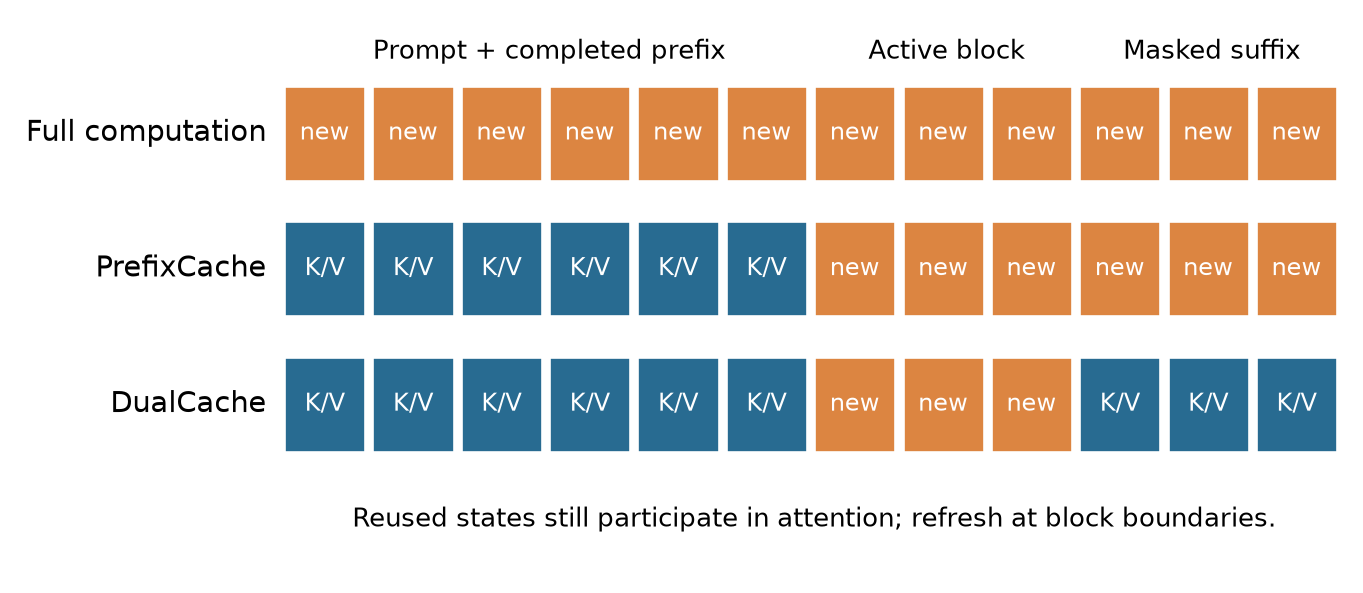
The paper’s similarity visualizations support the idea that K/V representations change gradually across nearby decoding steps. That is a useful empirical observation, but an average cosine similarity is not an error bound on output probabilities. A small change in a representation may affect a nearly tied token decision. Conversely, a relatively large representation change may leave the most probable token unchanged. The relevant question is how the approximation moves the distribution near decisions the policy will commit.

A subtle distinction is that the masked suffix is not semantically constant merely because its input tokens all remain MASK. Its contextual representation can change as the active block becomes visible. DualCache saves more recomputation by freezing those representations as well. That explains why it can offer a larger speedup and also why it is a more aggressive approximation.

Algorithm 1. Blockwise cached decoding

This pseudocode makes refresh and commitment explicit; it summarizes the paper’s method rather than prescribing a particular software implementation.

Input: prompt, answer length L, block size B, selection rule
1. Append L mask tokens to the prompt.
2. Initialize K/V states with a full-context computation.
3. For each answer block from left to right:
4.   While the current block contains masks:
5.     PrefixCache: recompute current block and suffix;
6.     DualCache: recompute current block only.
7.     Let queries use both fresh and cached K/V states.
8.     Compute predicted tokens and their confidences.
9.     Select masked positions with Algorithm 2 or 3.
10.    Commit the selected tokens together.
11.  Refresh the cached regions before the next block.
12. Return the completed answer.

The refresh operation must update representations, not merely append the newly completed token IDs. Otherwise the old prefix would remain tied to an increasingly outdated context. The paper’s multimodal extension later changes the refresh arrangement because short blocks can damage visual reasoning; block size is therefore not a universally transferable optimum.

4. Why marginal predictions can disagree jointly

Suppose two masked positions have a joint distribution over binary tokens. Consider the following deliberately small example, constructed for this review:

$$p(0,0)=0.32,\quad p(0,1)=p(1,0)=0.34,\quad p(1,1)=0. \tag{4}$$

Each position individually prefers zero with probability 0.66. Independent greedy decisions therefore choose (0,0), although either (0,1) or (1,0) is more likely under the joint distribution. Worse, independent sampling assigns positive probability to (1,1), which the joint model declares impossible. Correct marginals alone do not preserve combinations.

Let q be the product of those marginals. Then q(0,0)=0.4356, q(0,1)=q(1,0)=0.2244, and q(1,1)=0.1156. The total variation distance is 0.2312. This number is obtained by summing the four absolute differences and dividing by two; it is a property of the toy distribution, not a measured Fast-dLLM error.

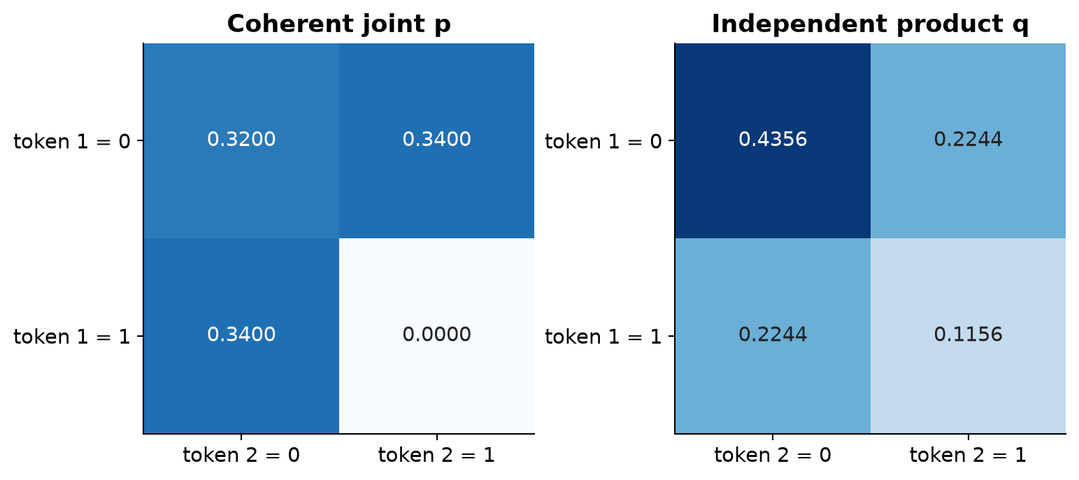
This is the motivation for confidence-aware selection. It is not enough that a token be the highest-scoring option at its position. Its probability must be sufficiently concentrated, relative to the number of positions committed together. Taking the top eight positions every time ignores whether their confidences are 0.99 or 0.55. A threshold adapts to the uncertainty of the particular decoding step.

Algorithm 2. Threshold selection with guaranteed progress

The fallback prevents the decoder from stalling when every confidence is below the threshold.

Input: masked positions M, probability vectors, threshold tau
1. For each i in M, choose token y_i with maximum probability.
2. Set c_i to the probability of y_i.
3. Select S = {i in M : c_i >= tau}.
4. If S is empty, select the position with maximum c_i.
5. Commit y_i for every i in S simultaneously.

The fallback guarantees at least one token of progress; it does not certify correctness. Likewise, passing a threshold does not verify a sampled answer against an external judge. This method alters the generative trajectory directly. It has a different quality contract from speculative decoding with a target-model verification and correction rule.

5. Deriving the confidence theorem without changing its meaning

Fix one context E and a coherent joint distribution p over n selected token positions. Let x_j^* be the preferred token at position j, with marginal probability greater than 1-epsilon. Define the independent approximation as

$$q(x\mid E)=\prod_{j=1}^{n}p_j(x_j\mid E),\qquad p_j(x_j^*\mid E)>1-\epsilon. \tag{5}$$

The word coherent is essential: all the marginals must come from the same joint distribution. Appendix A explicitly acknowledges that actual masked model predictions need not satisfy this idealized assumption exactly. The theorem is a statement about distributions with that property, not a proof that an arbitrary neural predictor has it.

First, if epsilon is at most 1/(n+1), each selected token has probability greater than one half for n>=1. Each coordinate is consequently the unique marginal maximizer, and their concatenation uniquely maximizes q. Second, a union bound lower-bounds the probability of the whole selected sequence:

$$p(x^*\mid E)=1-\Pr\left(\bigcup_j\{X_j\ne x_j^*\}\mid E\right)>1-n\epsilon. \tag{6}$$

Third, any alternative z differs from x^* at some coordinate k. The probability of that whole alternative is no greater than the probability that coordinate k is wrong:

$$p(z\mid E)\le p_k(z_k\mid E)\le \Pr(X_k\ne x_k^*\mid E)<\epsilon. \tag{7}$$

It is therefore sufficient that 1-n epsilon >= epsilon. Combining the inequalities gives

$$(n+1)\epsilon\le1\quad\Longrightarrow\quad\operatorname*{argmax}_{x}p(x\mid E)=\operatorname*{argmax}_{x}q(x\mid E)=x^*. \tag{8}$$

This derivation explains the count dependence: a probability concentration adequate for two simultaneous choices may be inadequate for thirty-two. Figure 3 plots the corresponding confidence boundary n/(n+1). The strict marginal inequality in the theorem matters at the boundary; a practical rule using greater-than-or-equal-to a threshold should not silently substitute equality for a strict premise.

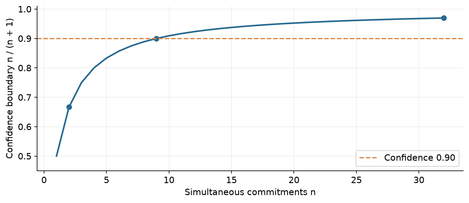
The theorem labels its first result as an equivalence for greedy decoding, but the displayed mathematical objects are joint and product-distribution maximizers. Joint MAP and ordinary sequential greedy decoding are not interchangeable in general. Under this strong concentration condition, a separate conditional argument can support sequential choices too: after fixing any subset of preferred tokens, the probability mass of the all-preferred sequence still dominates every event involving a particular wrong next token. The important point is that this extra reasoning uses the same coherent joint and concentration assumptions. It does not justify equating generic autoregressive greedy search with global MAP.

The condition is also a worst-case boundary rather than a necessary condition for every model. To see why a universal improvement is impossible, assign probability 1/(n+1)-eta to the all-zero string, and probability 1/(n+1)+eta/n to each of the n strings containing exactly one one. These probabilities sum to one. For a small positive eta, every coordinate still prefers zero, but a single-one string is more probable than all zeros. The two-token example in Section 4 is a concrete instance of this failure pattern.

5.1 A heterogeneous error budget

Here is a useful extension of the same argument, derived for this review. Suppose position j has error mass epsilon_j rather than a common bound. The union bound gives p(x*) >= 1-sum epsilon_j, while any alternative is bounded above by max epsilon_j. Thus a sufficient strict condition is

$$\sum_{j=1}^{n}\epsilon_j+\max_j\epsilon_j<1. \tag{9}$$

It can certify a group containing many extremely confident positions and one less certain position more effectively than replacing all errors by the largest one. This is a mathematical observation, not a policy evaluated by the paper. It would still inherit calibration and joint-consistency assumptions, and sorting by confidence alone need not optimize every cost-sensitive selection objective.

5.2 Distributional closeness is a separate guarantee

Agreement on the most probable sequence does not mean that the two distributions are identical. For n>1, Appendix A also bounds their distance. Write the norm order as r to avoid confusing it with the distribution p. The mass difference at x* is less than (n-1)epsilon. Away from x*, each pointwise difference is below epsilon, while the total tail absolute difference is below 2n epsilon. Therefore

$$\begin{aligned} \|p-q\|_r^r &< (n-1)^r\epsilon^r+\epsilon^{r-1}(2n\epsilon),\\ \|p-q\|_r &<\left((n-1)^r+2n\right)^{1/r}\epsilon,\\ \operatorname{TV}(p,q)&<\frac{3n-1}{2}\epsilon. \end{aligned} \tag{10}$$

These are worst-case bounds. If the right side of the TV expression exceeds one, it supplies no useful numerical guarantee beyond the universal TV maximum of one. A statement that the theorem permits a particular n is also not a statement that its TV bound is small enough for a sensitive downstream application.

The forward KL divergence has a particularly clear interpretation because q is the product of p’s own marginals:

$$\begin{aligned} D_{\mathrm{KL}}(p\|q) &=\sum_{j=1}^{n}H(X_j\mid E)-H(X_1,\ldots,X_n\mid E)\\ &=\sum_{j=2}^{n}I(X_j;X_1,\ldots,X_{j-1}\mid E). \end{aligned} \tag{11}$$

This is the dependence information removed by the independent approximation. Concentrating at least 1-epsilon mass on one token limits each marginal entropy. In the high-confidence range, spreading the remaining mass uniformly over V-1 other tokens maximizes entropy, yielding

$$D_{\mathrm{KL}}(p\|q)<(n-1)\left[h_b(\epsilon)+\epsilon\log(V-1)\right], \tag{12}$$

where h_b is binary entropy and V is vocabulary size. The argument requires the relevant high-confidence range in which this entropy upper bound increases with epsilon. It does not supply a reverse-KL bound. Indeed, in Figure 2, q assigns positive mass to a pair with p=0, so D_KL(q||p) is infinite. Direction matters when describing what has been controlled.

6. From the theorem to a practical selection rule

The factor strategy sorts masked positions by confidence c_(1)>=…>=c_(m) and chooses the largest n satisfying

$$(n+1)\left(1-c_{(n)}\right)<f. \tag{13}$$

The least confident selected token controls the common error bound. With f=1, this resembles the theorem’s sufficient condition if the model probabilities satisfy the theorem’s assumptions. Increasing f relaxes it. The appendix explores factors above one, so its fastest configurations deliberately move outside the literal worst-case guarantee.

Algorithm 3. Factor selection

The maximum-confidence fallback again ensures progress even if no multi-token group is admitted.

Input: masked positions, predicted tokens, confidences, factor f
1. Sort masked positions by decreasing confidence.
2. Search the candidate group sizes n = 1, ..., m.
3. Keep sizes satisfying (n + 1) * (1 - c[n]) < f.
4. Choose the largest admissible size.
5. If no size is admissible, choose the first position alone.
6. Commit the selected predicted tokens together.

A fixed threshold of 0.9 and a factor of one implement different policies. Thresholding can select every token in a large block if all clear 0.9. The theorem’s uniform bound with epsilon=0.1 only covers n<=9, assuming probabilities strictly exceed 0.9. A block with thirty-two such tokens is not certified by that argument. It may still work empirically because the bound is worst-case, but that is an empirical conclusion.

There is also a confidence-quality mismatch that cannot be solved by algebra alone. The network score is an estimate, and cache staleness can perturb it. Suppose, purely as an analysis assumption, that a selected token’s estimated marginal differs from its ideal marginal by at most delta. Then

$$\epsilon_{\mathrm{true}}\le 1-\widehat c+\delta,\qquad (n+1)(1-\widehat c+\delta)\le1 \tag{14}$$

would be the conservative sufficient test. Fast-dLLM does not provide such a delta certificate. Equation 14 identifies what is missing if one wants a calibrated guarantee; it does not assert that a usable bound has been measured. It also explains why evaluating confidence selection with fresh states and with stale states would be scientifically informative.

7. A cost model for the two complementary speedups

Two levers affect runtime: the number of forward evaluations and the cost of each evaluation. Let S be the number of denoising evaluations, C_full the cost of a full-context evaluation, C_active the cost with cached regions reused, and R the additional refresh cost. A rough explanatory model is

$$T_{\mathrm{base}}\approx S_0C_{\mathrm{full}},\qquad T_{\mathrm{fast}}\approx SC_{\mathrm{active}}+R+T_{\mathrm{selection}}. \tag{15}$$

This decomposition is not a fitted performance predictor. It helps explain why caching and parallel commitments can reinforce one another without producing an exact product of independently measured speedups. The changes also alter the sequence of states visited, output length, and which positions become confident together.

For the LLaDA GSM8K length-256 configuration shown in the paper’s Figure 1, throughput is 6.7 tokens/s for baseline, 21.2 for cache alone, 16.5 for parallel decoding alone, and 54.4 for their combination. Average tokens committed per step are 1, 1, 3.25, and 3.01 respectively. The combined method’s smaller tokens-per-step value does not negate its advantage: each step has become much cheaper.

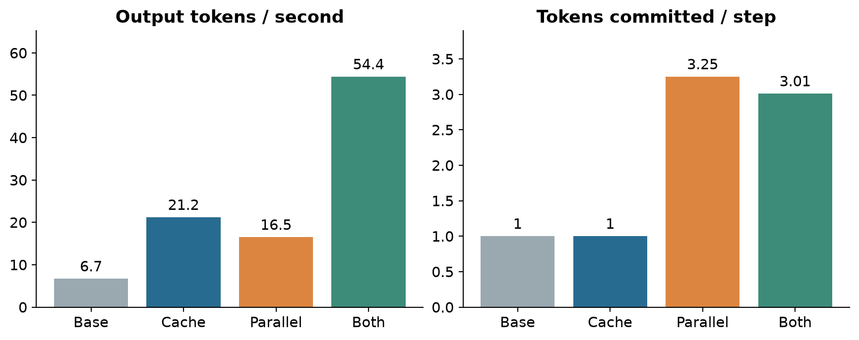
From the rounded throughput values, caching alone gives 3.16x, parallel decoding 2.46x, and the combined method 8.12x. Multiplying the two isolated ratios gives 7.79x. That discrepancy is not evidence of a violation of a runtime law; there is no such exact multiplicative law once trajectories and overhead change. A decomposition should be tested with per-request timing rather than inferred from four aggregate bars.

Finally, cached tokens still occupy memory and still participate as keys and values in attention. This paper is primarily about computation reuse, not about reducing the number of stored KV elements. It should not be grouped uncritically with eviction or low-bit KV compression methods merely because all three use the phrase KV cache.

8. Reading the main experiments as paired quality and speed results

The main experiments use an NVIDIA A100 80GB. The default configuration is PrefixCache with block size 32 and a confidence threshold of 0.9. GSM8K, MATH, HumanEval, and MBPP cover mathematical and coding outputs; LLaDA and Dream show that the method is not limited to a single diffusion backbone. These are useful axes of variation, although they do not establish portability to every model, serving stack, or batch regime.

The following selection of length-512 results reproduces the accuracy and throughput columns of Tables 1 and 2. Accuracy differences are percentage points, not relative percentages.

Model / task	Baseline accuracy	Fast accuracy	Baseline tok/s	Fast tok/s
LLaDA / GSM8K	77.5	77.2	3.2	35.3
LLaDA / MATH	37.2	36.0	8.0	47.1
LLaDA / HumanEval	43.9	44.5	18.4	73.7
LLaDA / MBPP	14.8	13.8	4.3	39.5
Dream / GSM8K	76.0	74.0	7.7	42.9
Dream / MATH	39.8	39.3	9.6	63.3
Dream / HumanEval	54.3	54.3	16.3	52.8
Dream / MBPP	55.6	55.2	9.4	73.6

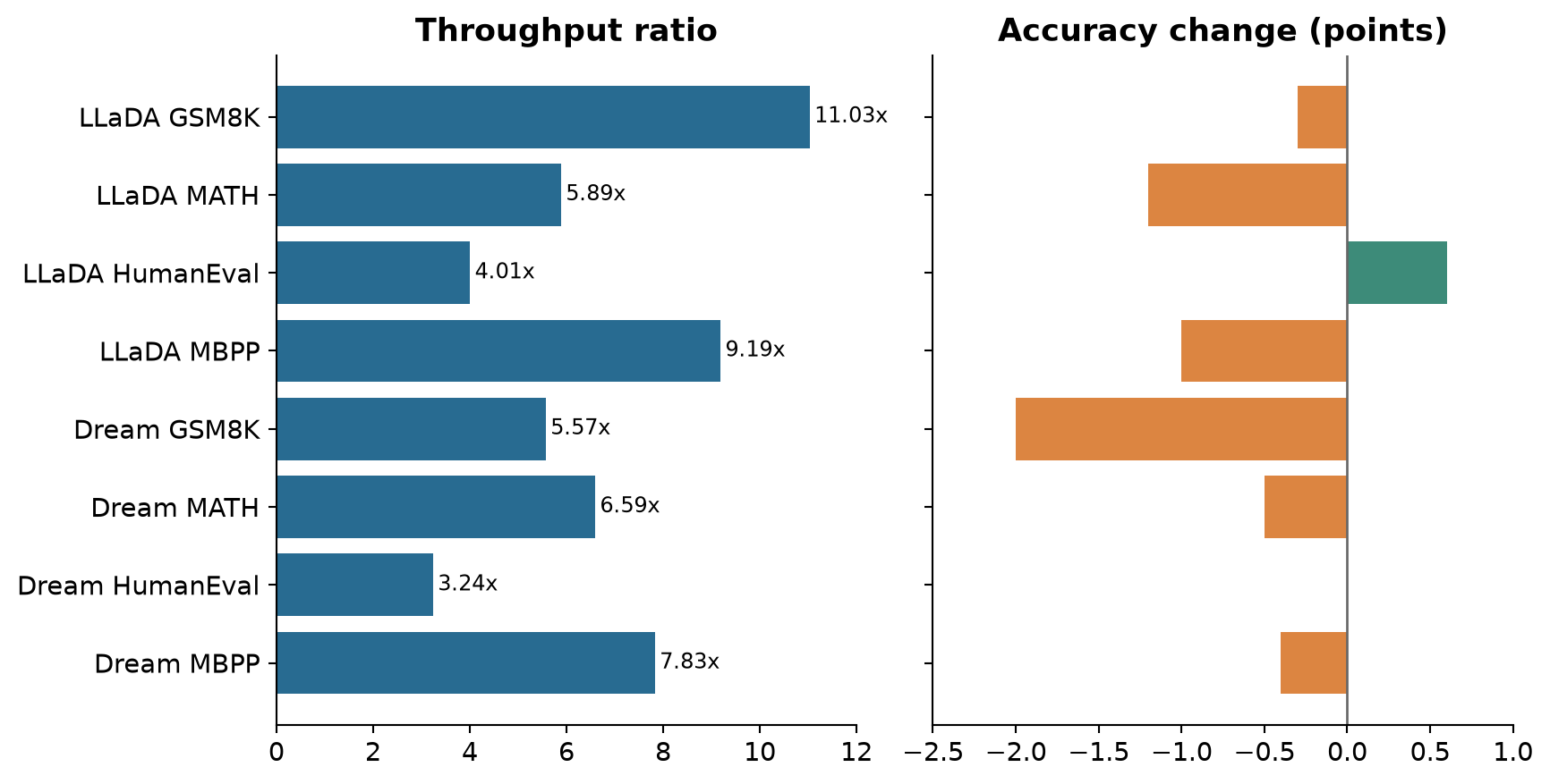
Several details prevent an overly simple reading. LLaDA’s MBPP accuracy is low at length 512 even before acceleration; a large relative throughput gain does not make that configuration a strong coding system. The small positive change on HumanEval is compatible with an altered decoding trajectory, but it is not by itself evidence that approximation improves general reasoning. No paired uncertainty estimate is supplied for each of these small differences.

The narrative says accuracies remain within one to two points of the backbone across settings. That is too broad as a literal summary. Dream length-256 HumanEval changes from 49.4 to 54.3 with the combined method, a 4.9-point increase. Its cache-only MBPP result changes from 56.6 to 53.2, a 3.4-point decrease. In the eight-shot, length-512 LLaDA ablation, DualCache moves 78.9 to 75.4. These exceptions do not erase the speed contribution, but a review should preserve the actual table entries.

There are also small ratio inconsistencies in Table 2. For Dream HumanEval at length 256, 62.0/23.3 is approximately 2.66, while the table labels the speedup 2.8x. For Dream MATH at length 512, 63.3/9.6 is approximately 6.59, while the label is 6.5x. I use the reported raw throughput values and identify calculated ratios as calculations. The available rounded values do not resolve whether the discrepancy comes from aggregation, rounding, or a table error.

9. The 27.6x result and the role of workload shape

Table 5 varies answer length under an eight-shot GSM8K prompt. It is particularly useful because it exposes the denominator of the headline result.

Answer length	Baseline tok/s	Parallel only	PrefixCache + parallel	DualCache + parallel
256	4.9	16.4	49.2	46.3
512	2.3	14.0	32.0	36.4
1,024	0.7	9.3	13.0	19.3

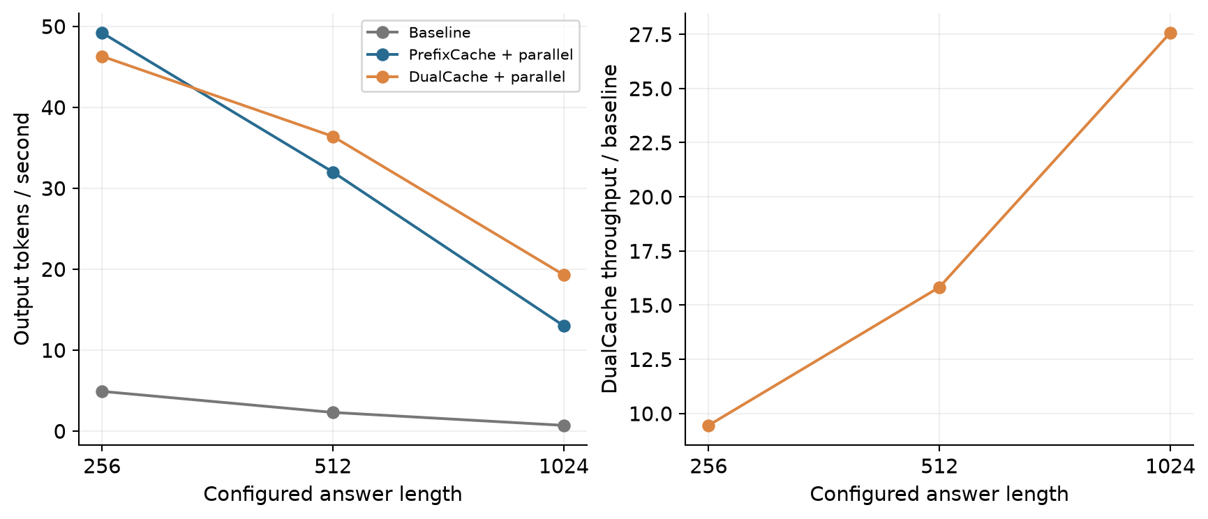
DualCache is not always faster than PrefixCache. At length 256 it reports 46.3 versus 49.2 tokens/s. At length 1,024 its advantage is clearer, 19.3 versus 13.0. Thus the statement that more caching is beneficial depends on how much expensive recomputation it avoids relative to its overhead and the resulting decoding trajectory.

The eight-shot length-1,024 accuracies are 77.3 for the baseline, 78.0 for parallel-only decoding, 75.7 for PrefixCache with parallel decoding, and 76.0 for DualCache with parallel decoding. The best-quality and best-throughput entries are different. In a five-shot length-1,024 configuration, DualCache reports 74.7 accuracy compared with a 77.0 baseline, again illustrating that the quality cost must accompany the acceleration number.

Figure 1c also labels end-to-end latencies of 266 seconds and 12 seconds for baseline and DualCache. Their rounded ratio is about 22.2, not 27.6. Because the paper defines throughput using generated output tokens until end-of-sequence, throughput and latency ratios can differ when generated lengths or averaging procedures differ. However, the published aggregates alone do not identify the exact explanation. I would request per-example lengths and times before claiming these two summaries have been reconciled.

For deployment decisions, the shape of the workload matters more than the largest reported ratio. A long few-shot prefix increases repeated context work that caching can save. A longer allocated masked answer can also depress the baseline substantially. A user facing a short answer task may care much more about the length-256 absolute speed and latency than about the maximum ratio in the longest setting.

10. More aggressive factors and the changing parallel frontier

The threshold policy and factor policy form different quality-speed frontiers. Table 11 compares the threshold baseline with a more aggressive factor strategy on LLaDA. The values below retain the paired accuracy differences.

Task / length	Threshold accuracy	Factor accuracy	Threshold tok/s	Factor tok/s
GSM8K / 256	78.5	77.5	54.4	78.5
GSM8K / 512	77.2	74.8	35.3	47.1
MATH / 256	33.2	32.0	51.7	78.3
MATH / 512	36.0	35.2	47.1	64.6

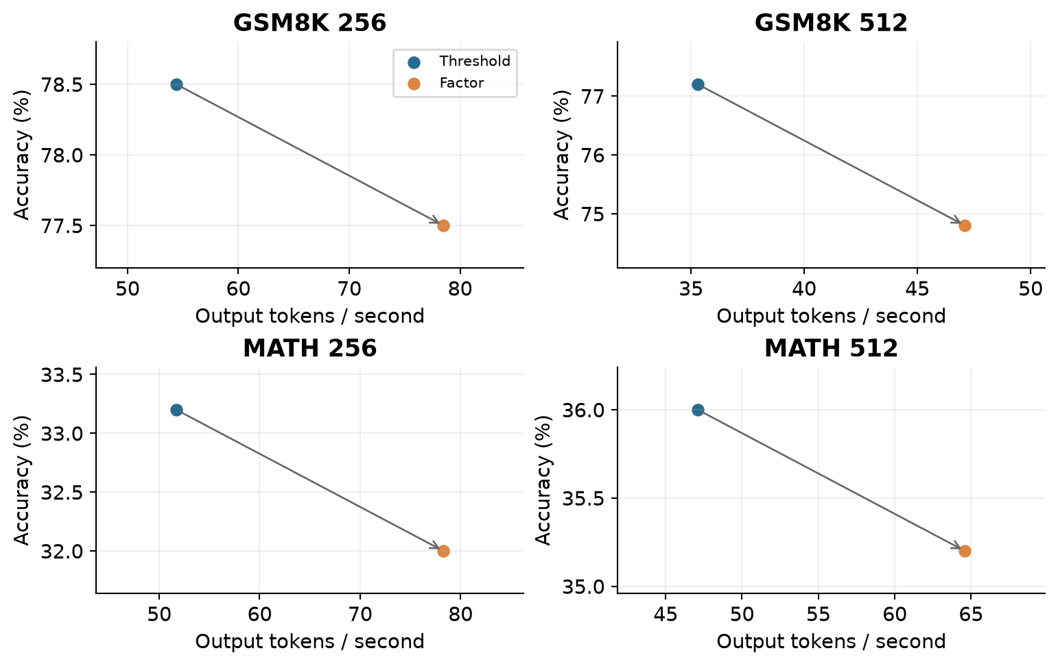
The factor strategy raises throughput by approximately 44%, 33%, 51%, and 37% in these four rows, calculated from the rounded values. It costs between 0.8 and 2.4 accuracy points. A prose summary of “40-50%” captures the rough scale but should not substitute for the individual comparisons. The fastest configuration is a selectable operating point, not an unconditional replacement for the default.

The paper’s Figure 5 shows another useful phenomenon: relaxing the threshold increases average tokens per step, from one at threshold 1.0 to 3.25 at 0.9 and 7.01 at 0.5 in that experiment. This supports adaptive commitment as a real source of fewer evaluations. It also shows why tokens-per-step alone is an incomplete optimization target. The least conservative point need not preserve the desired answer quality.

Figure 7 in the original paper examines token parallelism through the decoding trajectory, with higher parallelism in the middle than near the ends. An intuitive explanation is that some context must first be established, after which several positions become jointly easier. Late positions may contain unresolved difficult choices. But averaging by step can also change which examples remain in the sample: only unfinished trajectories contribute at late steps. Separating per-example behavior from this survivor effect would strengthen the interpretation.

11. Multimodal transfer reveals a real boundary

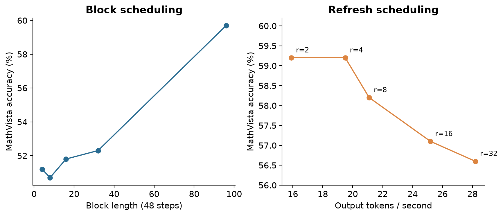
LLaDA-V is an important counterweight to the idea that a small block is always a safe setting. In Table 9, with 48 steps, MathVista accuracy is 59.7 at block length 96 but only 50.7 at block length 8. Throughput is about 5.6 versus 6.2 tokens/s. A modest throughput gain therefore accompanies a nine-point quality loss. The text attributes the sensitivity to visual reasoning’s need for global context.

The authors respond by preserving a full block and adjusting cache refresh intervals. Table 10 reports the following sequence: refresh intervals 2, 4, 8, 16, and 32 produce accuracies 59.2, 59.2, 58.2, 57.1, and 56.6, with throughputs 15.9, 19.5, 21.1, 25.2, and 28.2 tokens/s. This is a direct reminder that stale-state tolerance depends on both modality and the refresh policy.

In Table 3, Fast-dLLM reaches 56.6 on MathVista compared with a full-step baseline of 59.2, while throughput rises from 2.84 to 28.2 tokens/s. On MathVerse, it reports 28.6 versus 28.5, and 23.3 versus 2.75 tokens/s. The accuracy cost is therefore visibly task dependent even within the visual model. A single image-captioning example in the appendix illustrates latency reduction, but it cannot establish population-level preservation of visual reasoning.

The broader design lesson is to separate block scheduling from refresh scheduling. A block determines which positions are eligible to be filled; a refresh interval determines how long representations may remain stale. Treating both as one scalar “cache aggressiveness” obscures why the multimodal variant needs a different arrangement.

12. Batch scaling and alternatives

The appendix’s batch-scaling study uses cache-only decoding, without the confidence-aware parallel component. It varies batch size up to 32, with prefill length 256 and short generated lengths of 16, 32, and 64. For length 16 at batch 32, the text reports PrefixCache above 211 tokens/s versus about 43 for native LLaDA. This result concerns aggregate throughput in a particular short-generation batch setting. It must not be combined with the single-request 27.6x result as though they were two measurements of the same pipeline.

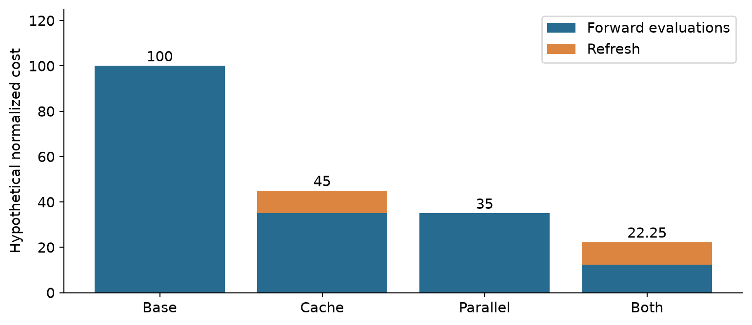
A simple normalized cost example helps organize the alternatives. Suppose a baseline uses 100 forward evaluations, each costing one unit. If caching reduces each to 0.35 and adds ten units of refresh cost, total cost becomes 45. If parallel selection alone reduces evaluations to 35, cost becomes 35. Combining those hypothetical assumptions gives 22.25 units. The result is a thought experiment about cost accounting, not an empirical estimate of any listed GPU.

An alternative is to train for blockwise generation so that the model distribution matches the intended inference structure. That can improve compatibility but gives up the paper’s training-free premise. Another is speculative decoding, where a parallel draft proposes tokens and an autoregressive target verifies them. That can preserve a target distribution under an appropriate correction rule, but adds a second model and verification overhead. Simply reducing diffusion steps is a third baseline; it often reduces work but does not selectively spend compute where confidence is low.

These alternatives optimize different contracts. A user who requires a specified target model’s output distribution should not treat approximate diffusion acceleration as interchangeable with verified speculation. A user who already uses a diffusion checkpoint and tolerates a measured quality-speed tradeoff may find training-free caching especially attractive.

13. Limitations and failure modes

The main uncertainty is not whether reuse can save compute; the tables demonstrate that. It is how reliably a setting chosen on one model and workload transfers to another. The experiments cover two text backbones and a visual variant on one stated GPU type. They do not establish a universally optimal block size, threshold, refresh interval, or serving batch policy.

The theoretical and empirical uncertainty are different. The theorem assumes coherent marginals and high concentration. The empirical decoder sees estimated probabilities, potentially derived from stale states, and commits tokens irreversibly. The paper supplies no general bound linking cache age to distributional error and no end-to-end guarantee that all future commitments preserve a baseline trajectory.

Reported accuracy changes also lack the paired uncertainty information needed to interpret every small gain or loss. A 0.2-point difference and a 3.5-point difference should not be described with the same confidence. Task composition, output length, and stopping behavior can influence average throughput. Sparse reporting of per-request timing makes it difficult to distinguish compute savings from changes in the output distribution.

Finally, the appendix’s LLaDA-1.5 results do not show uniform dominance. On length-512 MATH, the listed older Fast-dLLM configuration has accuracy 36.0 and throughput 47.1, while LLaDA-1.5 has 35.1 and 41.1. The newer backbone may help on other tasks, but the table should take priority over a blanket statement that it is always stronger and comparably fast.

14. Independent critical analysis

I regard the strongest contribution as identifying a useful separation between stable representations and uncertain commitments. The method avoids spending a full forward pass recomputing everything solely because one token remains uncertain. Its threshold rule also recognizes that uncertainty changes across positions and over time. These are convincing design principles even if the current confidence theorem does not certify a practical neural decoder.

The weakest explanatory link is the interaction between the two approximations. Cache staleness can change confidence; confidence determines how many tokens are committed; the resulting commitments change how quickly the cached context becomes obsolete. Evaluating cache and parallel decoding separately is informative, but does not isolate this feedback loop. A factorial experiment should cross fresh versus stale states with fixed versus adaptive selection while recording the same prompts and comparable stopping rules.

A particularly useful diagnostic would compare the cached and fresh distributions at positions immediately before commitment. Record the top-token agreement, confidence shift, and divergence as a function of cache age and block position. Then stratify final task accuracy by those diagnostics. This would test whether representation similarity actually predicts safe commitment, instead of assuming it does. These are proposed measurements, not reproduced results.

Algorithm 4. A proposed paired evaluation protocol

This is a research proposal for evaluating the method’s claims, not an evaluation performed in this review.

1. Fix prompts, model checkpoint, hardware, and output limits.
2. Run fresh-state and cached-state decoding on paired inputs.
3. Record per-request output length, time, and answer score.
4. At commitment points, compare fresh and cached predictions.
5. Stratify disagreements by cache age and token confidence.
6. Repeat threshold/factor settings and report uncertainty.
7. Plot quality against latency and aggregate throughput.
8. Keep batch-size studies separate from single-request tests.

The theorem also suggests a more direct ablation: compare the paper’s worst-selected-confidence rule with the heterogeneous bound in Equation 9. The latter may admit more tokens when most are exceptionally confident, but could be brittle to miscalibration. Measuring calibration before claiming a theoretical benefit would be necessary. A method based only on estimated marginals cannot infer arbitrary dependency structure from confidence alone.

For systems readers, the highest-value follow-up is not another largest-ratio headline. It is a quality-constrained throughput curve across prompt lengths, output lengths, and batch sizes, compared against relevant optimized baselines. The numerical discrepancy between throughput and latency summaries makes per-request reporting especially valuable. Fast-dLLM would remain an interesting result even if a fairer baseline reduced the headline multiplier, because avoiding redundant bidirectional computation is independently useful.

15. Conclusion

Fast-dLLM turns two properties of diffusion decoding into practical speed: nearby states can be similar enough to reuse, and some iterations contain several predictions confident enough to commit together. PrefixCache and DualCache reduce work per evaluation; threshold and factor policies reduce the number of evaluations. The reported gains are substantial and spread across multiple tasks, but their quality cost and magnitude depend on the workload.

The theorem gives a clean way to think about dependence: simultaneous commitments require a confidence budget that shrinks as their count grows. It does not eliminate the need to measure stale-state error, calibration, or end-to-end quality. My preferred takeaway is therefore a design pattern plus an experimental discipline: reuse stable computation, adapt commitment to uncertainty, and report absolute speed with the exact quality and workload that produced it.

References and reading scope

1. Wu et al. Fast-dLLM, arXiv:2505.22618v3. All 22 PDF pages read, including Appendix A’s proof, qualitative examples, and Appendix C’s additional experiments.
2. Author project page. Used to identify the official paper resources; numerical discussions above use the v3 PDF’s figures and tables.
3. The mathematical counterexample, heterogeneous sufficient condition, and normalized cost example in this review are explanatory derivations. Proposed evaluations in Section 14 have not been run and are not presented as replication evidence.