Scalable Kronecker-Fisher Approximation: What Cross-Layer Curvature Can Tell Us About Compression

Review date: 2026-09-26
Author: Zhongzhu Zhou
Paper reviewed: Scalable Kronecker-Fisher Approximation: Efficient Hessian Analysis for Billion-Parameter Language Models Compression
Paper authors: Viacheslav Yusupov, Daria Cherniuk, Evgeny Frolov
arXiv: 2609.02451v1, submitted September 2, 2026
this review follows the complete 12-page v1, including Appendices A-C.

1. The question that makes this paper worth reading

When a compression method assigns a score to each layer independently, it assumes that the scores remain useful after several layers change together. That assumption is convenient and often effective. It is also incomplete: a value projection can change the representation that a later feed-forward projection receives. Two individually acceptable modifications can become a poor combination, while a compensating modification can reduce damage elsewhere.

I read this paper as an attempt to make those relationships visible without constructing a matrix with one row and column per model parameter. Its central object is an empirical gradient second moment, represented by a short sum of Kronecker products plus a separately stored diagonal. The representation retains entries between different parameter groups; it is not restricted to a separate approximation for every layer.

There are three distinct contributions to keep apart. First comes a representation and a matrix-free way to estimate it. Second comes a descriptive account of which layer types are sensitive to quantization and sparsification. Third comes the proposal that coupling helps choose where to repair a damaged model. The first is a mathematical construction; the latter two require empirical validation. A compact representation alone does not establish that its brightest blocks predict every compression decision.

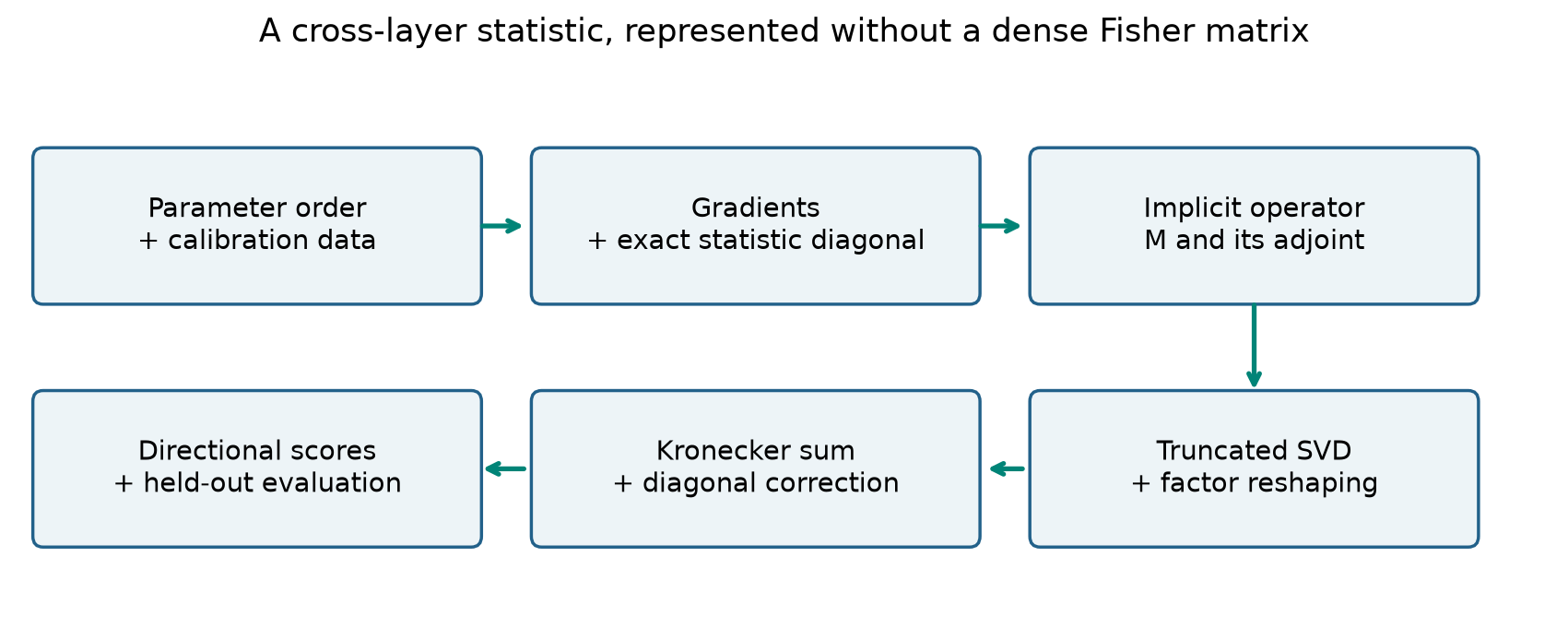
The paper is a useful follow-up to layerwise Fisher-weighted SVD. It asks about the information that independent decompositions discard. It does not present a complete, benchmark-winning joint rank-allocation system. I will therefore distinguish a diagnostic tool from an end-to-end compression policy throughout this review.

My main reservation concerns the measurement scale. The paper subtracts individual perplexity increases from a joint perplexity increase and interprets the residual as evidence of interaction. Because perplexity is exponential in mean negative log likelihood, that residual can be positive even when negative log likelihood is exactly additive. I derive this point later; it narrows the causal interpretation without denying the reported degradation.

2. Prerequisites: a loss surface has directions and couplings

2.1 A second-order model of compression

Let $w\in\mathbb R^d$ contain the selected parameters, and let $\delta$ be the change made by compression. For a differentiable evaluation loss $L$, a local expansion gives

$$L(w+\delta)-L(w) =\nabla L(w)^\top\delta+\frac12\delta^\top H\delta +O(\|\delta\|^3). \tag{1}$$

Here $H=\nabla^2L(w)$ is the Hessian. Near a stationary point, the linear term may be small. That does not make the remainder small for arbitrary quantization errors: locality is a separate assumption. Four-bit quantization and removing half of a layer’s weights are finite changes, not infinitesimal probes.

Partition $\delta$ into changes $\delta_P$ and $\delta_Q$ in two parameter groups. The quadratic term expands as

$$\frac12\delta^\top H\delta =\frac12\delta_P^\top H_{PP}\delta_P +\frac12\delta_Q^\top H_{QQ}\delta_Q +\delta_P^\top H_{PQ}\delta_Q, \tag{2}$$

assuming $H_{QP}=H_{PQ}^\top$. The last term is what block-diagonal reasoning removes. It depends on the directions of the actual errors, not just on the number of weights in the groups. Even a large block norm does not tell us the sign of that contribution.

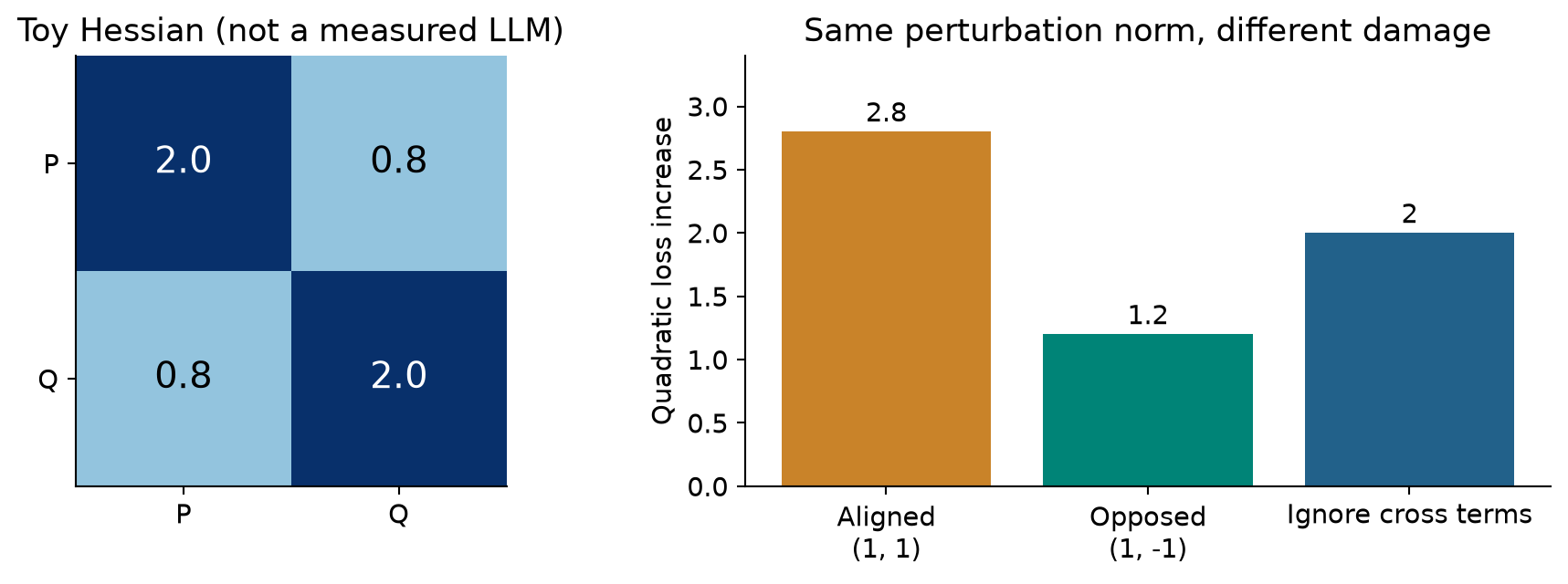
For an explicit example, take

$$H=\begin{pmatrix}2&0.8\\0.8&2\end{pmatrix}. \tag{3}$$

The quadratic damage is $2.8$ for $\delta=(1,1)$ and $1.2$ for $\delta=(1,-1)$. Ignoring the off-diagonal entries predicts $2$ for both. These are exact values of a toy quadratic, not measurements on a language model. They show why the same apparent layer sensitivities can produce different joint outcomes.

2.2 Three matrices that should not be merged conceptually

The empirical Fisher is a gradient outer-product statistic:

$$J=\mathbb E_{x\sim\mathcal D}[g_xg_x^\top], \qquad g_x=\nabla_w\ell(w;x). \tag{4}$$

It is positive semidefinite because $z^\top Jz=\mathbb E[(g_x^\top z)^2]\geq0$. The true Hessian need not have that property away from a suitable local minimum. A model Fisher additionally involves labels drawn from the model distribution, rather than necessarily using the observed labels in $\mathcal D$. Those distinctions matter even if all three matrices are called curvature in informal discussion.

The paper uses the empirical Fisher as a Hessian proxy and motivates the substitution by a converged pretrained model. I treat this as a modeling assumption. Stationarity by itself is insufficient to prove equality. For a scalar squared-error model with every residual exactly zero at a fitted solution, every sample gradient can be zero, so the empirical Fisher is zero, while the Hessian is positive. A local optimum is therefore not a general identity theorem.

This distinction helps interpret the validation. Agreement with the true Hessian on a small model is evidence about that setting; keeping more terms in an empirical-Fisher approximation cannot automatically remove a discrepancy between the empirical Fisher and the true Hessian.

3. Rearrangement: low rank in a different matrix

3.1 An index-based derivation

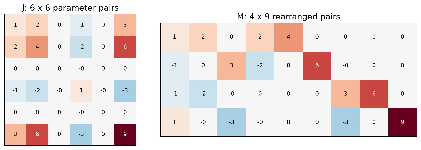
Choose a parameter ordering and reshape a gradient into $G\in\mathbb R^{n\times m}$ with $nm=d$. To avoid ambiguity about commutation matrices, I use row-major paired indices in this explanation: parameter $(i,a)$ corresponds to $G_{ia}$. A different vectorization convention gives the same construction after consistent permutations.

The gradient second moment has entries

$$J_{(i,a),(j,b)}=\mathbb E[G_{ia}G_{jb}]. \tag{5}$$

Rearrange these entries into a matrix $M$ whose row index is $(i,j)$ and column index is $(a,b)$:

$$M_{(i,j),(a,b)}=J_{(i,a),(j,b)}. \tag{6}$$

Then $M$ has shape $n^2\times m^2$ and equals $\mathbb E[G\otimes G]$ under this convention. Rearrangement preserves the collection of entries and thus the Frobenius norm. It is not generally a similarity transformation: dimensions can differ, and eigenvalues need not be preserved.

Write the singular value decomposition

$$M=\sum_{s=1}^{R}\sigma_su_sv_s^\top. \tag{7}$$

Reshape $u_s$ into $U_s\in\mathbb R^{n\times n}$ and $v_s$ into $V_s\in\mathbb R^{m\times m}$. Since a single outer product has entries $(U_s)_{ij}(V_s)_{ab}$, undoing the rearrangement gives

$$J=\sum_{s=1}^{R}\sigma_s(U_s\otimes V_s). \tag{8}$$

This is an exact decomposition when all terms are retained. The approximation keeps only $r$ terms. The important distinction is that $r$ counts Kronecker terms, not the ordinary matrix rank of $J$. One term $U\otimes V$ can have rank $\operatorname{rank}(U)\operatorname{rank}(V)$, potentially full rank in parameter space.

3.2 What is optimal, and what is not

Truncated SVD minimizes $\|M-M_r\|_F$ among matrices of ordinary rank at most $r$. Through the rearrangement, it minimizes the corresponding Frobenius error among representations with at most $r$ unrestricted Kronecker terms. The squared residual equals the sum of discarded squared singular values:

$$\|J-J_r\|_F^2=\|M-M_r\|_F^2 =\sum_{s>r}\sigma_s^2. \tag{9}$$

That guarantee is about fitting the chosen statistic, with the chosen reshape. It is not an optimality guarantee for compression accuracy, for a true-Hessian approximation, or for a memory-limited algorithm with additional positivity constraints. Changing the ordering can change how compactly the matrix is represented at a fixed term count.

For a particular perturbation, the error in quadratic damage is bounded by

$$\left|\frac12\delta^\top(J-J_r)\delta\right| \leq\frac12\|J-J_r\|_2\|\delta\|^2 \leq\frac12\|J-J_r\|_F\|\delta\|^2. \tag{10}$$

This supplies intuition but not a tight guarantee for every proposed compression. A small average entrywise error can still obscure an important direction. The right evaluation is ultimately whether the approximation ranks the perturbations we might actually choose.

4. Matrix-free estimation and the meaning of an exact diagonal

4.1 The operator can be applied without being stored

The rearranged matrix remains enormous. The paper instead supplies a routine that multiplies a vector by it. For $V\in\mathbb R^{m\times m}$, expanding an output entry gives

$$[\mathcal M(V)]_{ij} =\mathbb E\sum_{a,b}G_{ia}V_{ab}G_{jb} =[\mathbb E(GVG^\top)]_{ij}. \tag{11}$$

Its adjoint, defined by the Frobenius inner product, is

$$\mathcal M^*(U)=\mathbb E[G^\top UG]. \tag{12}$$

Indeed, $\operatorname{tr}(U^\top GVG^\top)=\operatorname{tr}((G^\top UG)^\top V)$. These two routines provide the information a truncated singular-value solver needs. The paper uses an implicitly restarted Arnoldi method. That choice avoids dense storage; it does not make the products free.

An iterative solver must repeatedly see the same operator. Recomputing statistics on independently shuffled or randomly augmented samples at every product would instead expose a changing matrix unless the algorithm is explicitly designed for stochastic products. Caching gradients and replaying a fixed calibration stream are two possible strategies, with different memory and computation costs. The article does not fully specify this engineering tradeoff; it should remain visible in a cost interpretation.

4.2 Diagonal replacement is an additional approximation decision

Let $d_J=\mathbb E[g\odot g]$. The construction can be written explicitly as

$$\widetilde J=J_r+ \operatorname{Diag}\big(d_J-\operatorname{diag}(J_r)\big). \tag{13}$$

This replacement ensures that each diagonal entry matches the gradient statistic being estimated. For any fixed $J_r$, it removes its diagonal squared error relative to that statistic while leaving off-diagonal error unchanged. It does not establish exact true-Hessian diagonals. Nor does it preserve the earlier claim that the result belongs to the class of only $r$ Kronecker terms: there is now a separate diagonal component.

The repair is practical because the diagonal needs only $d$ entries and can be accumulated while collecting gradients. Its contribution to a score is cheap:

$$\delta^\top\widetilde J\delta =\delta^\top J_r\delta+ \sum_t\left[(d_J)_t-(J_r)_{tt}\right]\delta_t^2. \tag{14}$$

There is a subtle statistical boundary here. The paper introduces per-sample gradients but describes its operator using gradients accumulated over batches. If a batch gradient is the mean of $b$ independent sample gradients, then

$$\mathbb E[\bar g\bar g^\top] =\mu\mu^\top+\frac1b\operatorname{Cov}(g), \qquad \mathbb E[gg^\top]=\mu\mu^\top+\operatorname{Cov}(g). \tag{15}$$

Thus averaging gradients before squaring differs from averaging their outer products. At $\mu=0$, the discrepancy is a scale factor under independent sampling; away from that condition it also changes relative components. Correlated sequence tokens further complicate the interpretation. “Exact diagonal” should therefore mean exact for a clearly specified finite-sample statistic and loss reduction.

4.3 Algorithm 1: assemble a usable representation

The following is explanatory pseudocode for Section 3, with bookkeeping conditions made explicit. It is not a claim about unreported implementation details.

01 Fix weights, parameter order, reshape (n,m), data and loss reduction.
02 Collect or deterministically replay the chosen gradient samples g_b.
03 Accumulate d_J = mean_b(g_b elementwise squared).
04 Define M(V)  = mean_b(G_b V G_b^T).
05 Define Mt(U) = mean_b(G_b^T U G_b).
06 Use M and Mt in a singular solver; retain r singular triplets.
07 Reshape left/right singular vectors into U_s and V_s.
08 Store sigma_s and factors, without expanding Kronecker products.
09 Store d_J minus the diagonal of that sum as a correction vector.
10 Report residuals, calibration convention and parameter scope.
11 Check held-out scores and actual compressed-model behavior.

Each step has a reason. Ordering makes the factorization reproducible. The adjoint enables a correct rectangular singular problem. Diagonal correction protects coordinatewise statistics. Held-out checks distinguish a good matrix fit from useful compression guidance. A failed solver tolerance or ambiguous sample convention is not fixed by drawing a more convincing heatmap.

5. Reading the representation: validation, visualization, and cost

5.1 The small-model check is informative but modest

The exact-Hessian experiment uses a two-layer perceptron with input and output dimensions 500 and hidden dimension 8, approximately 8,000 parameters, trained on a synthetic dataset of 500 Gaussian clusters. The paper uses binary cross entropy and AdamW. This is a setting where constructing the true Hessian is feasible.

Table 1 reports the following score:

$$R_{\mathrm{paper}}^2 =1-\frac{\|H-\widetilde J\|_F^2}{\|H\|_F^2}. \tag{16}$$

The denominator is the squared norm of $H$, not a mean-centered total sum of squares. I use the paper’s label but do not interpret it as the usual centered regression coefficient of determination. At 16 terms, the score is 42.3% with diagonal replacement and 29.9% without it. The improvement is 12.4 percentage points; the remaining squared residual in the former case is still 57.7% of $\|H\|_F^2$.

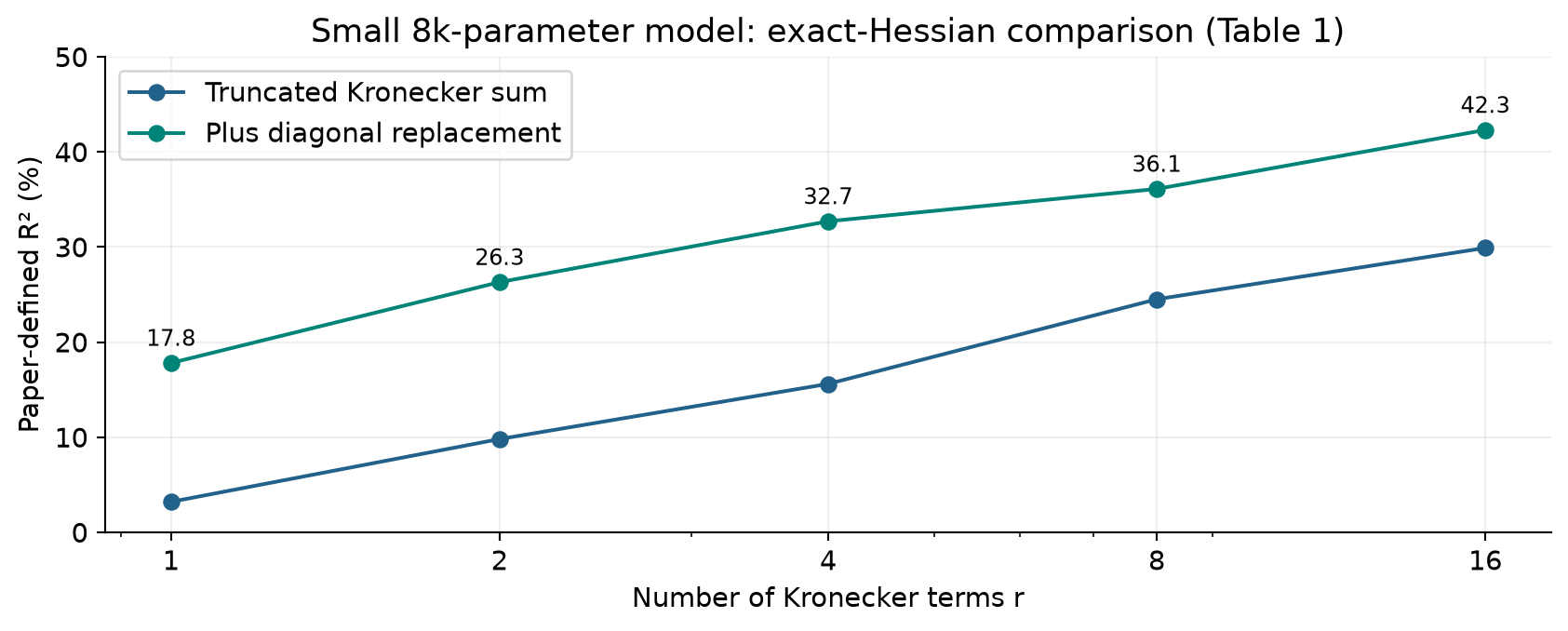
The rank sweep supports retaining the diagonal, especially at small $r$. It does not isolate all error sources. The total discrepancy combines the empirical-Fisher substitution, finite calibration, truncated Kronecker representation, and numerical solver error. A better presentation would compare both against the sample Fisher and against the true Hessian, so readers could see which gap each additional term closes.

5.2 A compressed heatmap is a summary of a summary

For a block indexed by $(i,j)$, the approximation has the form $\sum_s\sigma_s(U_s)_{ij}V_s$. Averaging all entries of that block gives

$$(J_{\mathrm{vis}})_{ij} =\sum_s\sigma_s(U_s)_{ij} \left(\frac1{m^2}\sum_{a,b}(V_s)_{ab}\right), \quad i\neq j. \tag{17}$$

The displayed diagonal uses the average of exact coordinate diagonals in the corresponding group instead. Consequently, a diagonal pixel and an off-diagonal pixel summarize different sets of entries. They should not automatically be compared as if each represented the same block norm.

Signed means can also cancel. The matrix $\begin{pmatrix}1&-1\\-1&1\end{pmatrix}$ has mean zero but Frobenius norm 2 and a nonzero action on $(1,-1)$. A dim block is not proof of no consequential coupling. The paper’s heatmaps are useful exploratory views; direction-sensitive scores or complementary absolute-value/norm summaries would strengthen a selection rule.

Appendix A shows groups of OPT-350M blocks 4-6, 8-10, and 20-22, with weaker values in the later group, as well as a full-model OPT-125M view. This is evidence about depth structure in those examples. It does not establish an invariant parameter ordering or a universal late-layer compression policy.

5.3 Linear representation memory has important constants

The factors store $r(n^2+m^2)$ entries, and the separate diagonal stores $d=nm$. For balanced dimensions,

$$n\approx m\approx\sqrt d \quad\Longrightarrow\quad r(n^2+m^2)+d\approx(2r+1)d. \tag{18}$$

Balance minimizes $n^2+m^2$ for a fixed product, since $(n-m)^2\geq0$. This explains the reshape choice. It also shows why “linear in parameters” does not mean the same size as the parameter vector. At $d=10^9$ with four bytes per entry, the representation alone is roughly 12 GB for $r=1$ and 132 GB for $r=16$, using decimal units. These are analytic counts, not measured GPU peaks.

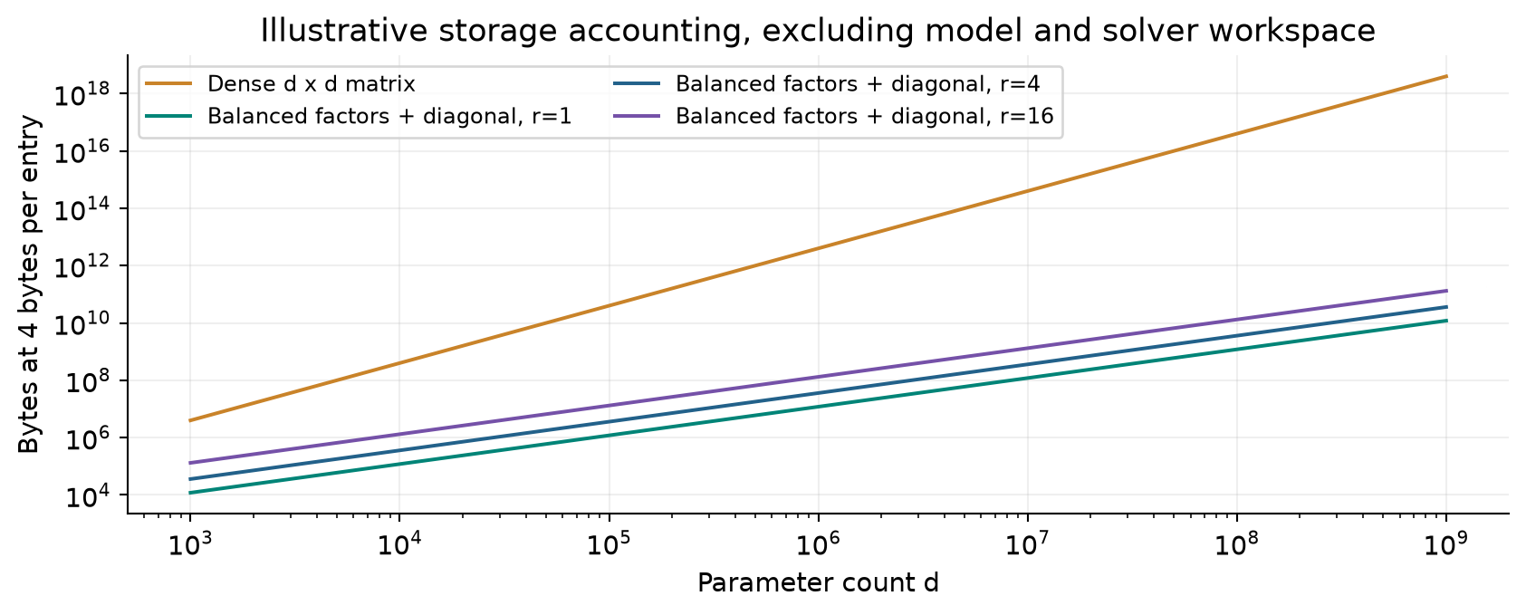
The matrix products cost $O(Bd(n+m))$ per iteration over $B$ gradient samples. With $N_A$ iterations and $T$ tokens per batch, the paper’s simplified time model becomes

$$O\!\left(Bd[T+N_A(n+m)]\right) \approx O\!\left(Bd[T+N_A\sqrt d]\right). \tag{19}$$

The resulting time is not linear in $d$ under a balanced reshape. Moreover, storing all $B$ gradients requires an additional $O(Bd)$ term; regenerating them trades storage for repeated work. Treating $B$ and solver workspace as constants is legitimate for an asymptotic statement but insufficient for a practical peak-memory claim.

6. The measured workload and the compression evidence

6.1 Construction time is not inference acceleration

Table 2 measures a rank-one approximation over all Transformer blocks, using 20 batches of 10 WikiText2 sequences on one H100. It reports 157.64 seconds for OPT-125M, 1,563.07 for OPT-350M, 1,090.61 for Qwen2-0.5B, and 2,428.25 for OLMo2-1B. The gradient portions are respectively 50.73, 272.94, 200.09, and 218.64 seconds.

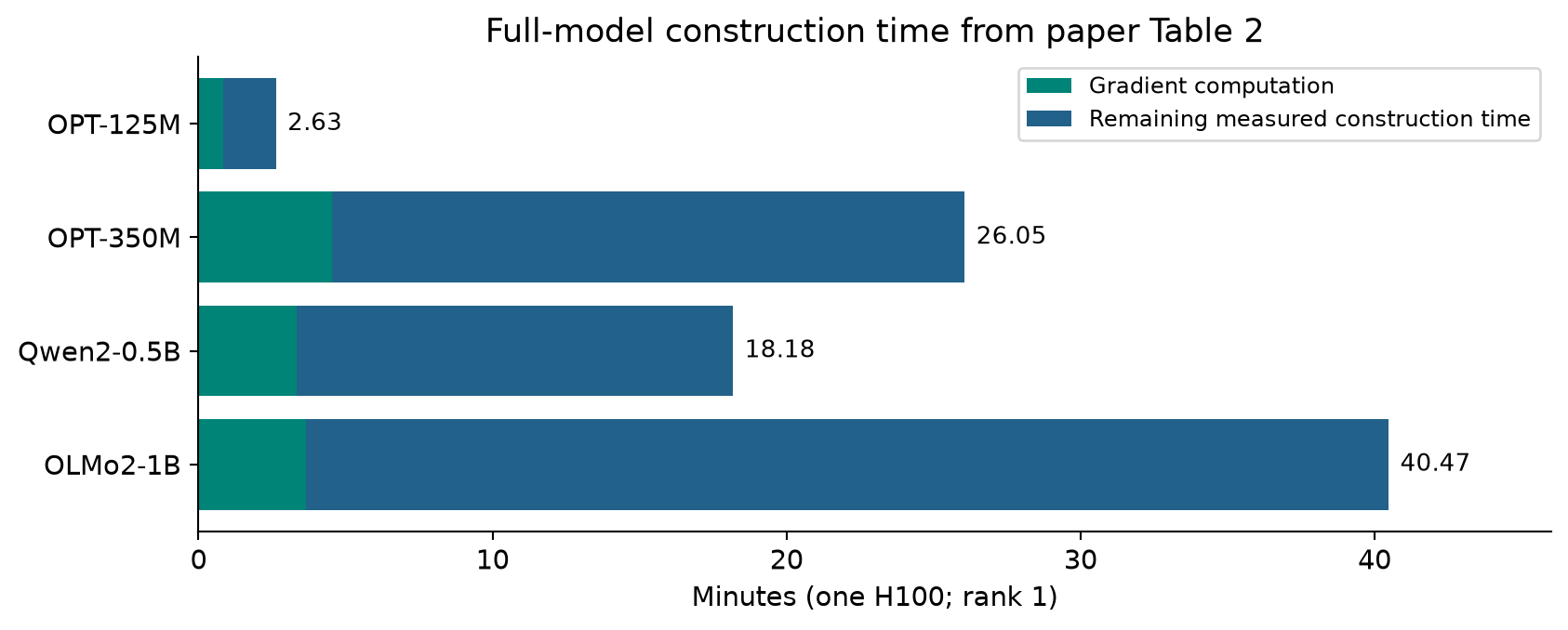
OLMo2-1B takes about 40.47 minutes, and gradient computation is about 9.0% of its total. That supports feasibility for the reported setup. It does not show that a 7B full-model approximation takes less than an hour, because no 7B timing row is provided. Nor does a rank-one timing establish the cost of the rank-16 small-model configuration.

The nonmonotone timing between OPT-350M and Qwen2-0.5B also warns against fitting a universal time curve from parameter count alone. Matrix shape, selected parameters, sequence length, numerical convergence, and execution details can matter. I would want these controls and measured peak memory before making a deployment budget.

The estimator prepares information that may help a later compressor. It does not by itself reduce generation latency or weight memory in the deployed model. Savings should be assessed only after a compression policy uses the statistic and produces a measured model.

6.2 What is actually perturbed

The main corruption experiments cover OPT-350M, Qwen2-0.5B, OLMo2-1B, and Qwen2.5-7B. They apply uniform four-bit quantization or 50% sparsification to a selected layer type across the middle Transformer blocks, excluding the first and last three blocks, and measure WikiText2 perplexity.

“One layer” therefore often means a family of projections across many blocks, rather than one physical matrix. This matters when interpreting inter-layer claims. Both within-block and across-block effects can contribute when all middle value projections change together. The experiment establishes the behavior of the selected group.

The first and last blocks are excluded because the paper observes different boundary behavior and weaker correspondence. That is a reasonable diagnostic scope, but the resulting ranking does not directly cover a compressor that must process every block. The boundary exclusion should remain part of any claimed operating range.

There is also a naming discrepancy worth preserving: Figure 2 labels the small Qwen visualization as Qwen2.5-0.5B, while the experiment descriptions, later plots, and tables use Qwen2-0.5B. I retain the labels of each result and do not silently assume that the checkpoints are interchangeable.

6.3 Per-parameter sensitivity and total damage answer different questions

Figure 3 divides perplexity growth by the number of modified parameters. Under that normalization, value projections are highly sensitive. OLMo2’s down projection leads under quantization, while its value projection leads under sparsification. The authors themselves discuss how the smaller value projection can receive a larger per-parameter score.

A per-parameter metric estimates something like damage density. A policy with a total memory budget needs both damage and bytes saved. If one family has a larger raw loss increase but vastly more parameters, it may still offer a useful tradeoff. Conversely, a compact but fragile projection may be cheap to retain. Neither raw damage nor normalized damage alone solves the allocation problem.

The pairwise figures use unnormalized perplexity growth, so their color intensities cannot be compared directly with the normalized bars. Large layers can dominate joint damage simply by size. Separating these two protocols is necessary before attributing a bright pairwise cell to stronger statistical coupling.

7. Joint damage and repair: what the numbers support

7.1 Reconstructing the pairwise residual

The paper defines an interaction difference using perplexity increases:

$$D_I(P,Q)=\Delta_{\mathrm{PPL}}(P,Q) -\Delta_{\mathrm{PPL}}(P)-\Delta_{\mathrm{PPL}}(Q). \tag{20}$$

Appendix B’s Figure 11 supplies numerical values, allowing a more concrete reading than a heatmap alone. For OPT-350M, value-only corruption increases perplexity by 1.283, FC1-only by 2.373, and their joint corruption by 4.743. Subtracting the displayed values gives $1.087$. For O plus FC1, the corresponding residual is $3.028-0.346-2.373=0.309$.

The same operation gives $-0.033$ for OPT’s Q/K pair and $0.939$ for its FC1/FC2 pair. The signs are not uniformly positive. These calculations use rounded values printed in the paper, so their last digits should not be presented as more precise than the source.

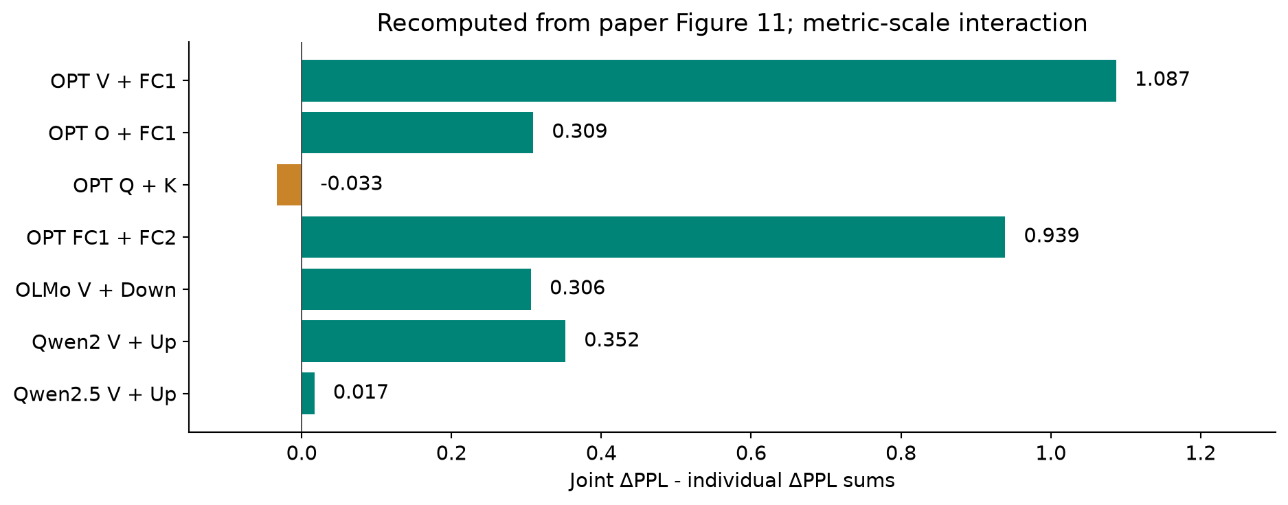
For OLMo2, value plus down gives $2.535-0.609-1.620=0.306$. Qwen2’s value/up residual is $0.352$, while Qwen2.5-7B’s is $0.017$. Different base perplexities and different perturbations make cross-model numerical comparison hazardous. The plot is an accounting exercise that grounds the discussion, not evidence that one architecture is universally more coupled.

The O projection is a revealing failure case. The estimated curvature view gives relatively low O-region values, yet joint corruption involving O can be damaging. The authors hypothesize that finite perturbations disturb residual-stream outlier channels that a local gradient statistic misses. That explanation is plausible, but it is proposed, not established by a controlled mediation experiment.

7.2 Why coupling can suggest a repair location

The recovery experiments first damage MLP projections, then fine-tune one attention projection type at a time. Figures 7 and 8 show full fine-tuning and LoRA results for the plotted Qwen2-0.5B and OLMo2-1B cases. Value adaptation recovers more than Q or K adaptation in those plots. I do not infer exact unprinted bar values or claim that the displayed recovery study covers all four model families.

A local quadratic model explains the intuition. Let $e_C$ be a fixed compression error in group $C$, and $z_R$ be a repair in group $R$. Ignoring the original linear term, the relevant objective is

$$q(z_R)= \frac12e_C^\top H_{CC}e_C +z_R^\top H_{RC}e_C +\frac12z_R^\top H_{RR}z_R. \tag{21}$$

If $H_{RR}$ is positive definite, differentiating gives

$$z_R^*=-H_{RR}^{-1}H_{RC}e_C. \tag{22}$$

Substitution shows that the best achievable reduction in this model is

$$\frac12e_C^\top H_{CR}H_{RR}^{-1}H_{RC}e_C. \tag{23}$$

This is my explanatory derivation, not a theorem asserted or tested by the paper. It says more than “pick the largest cross block.” Repairability also depends on the local curvature of the repair group, the direction of the corruption, and the available update subspace. If LoRA constrains $z_R$, only part of the ideal update may be expressible.

For a scalar illustration, take $H_{CC}=2$, $H_{RR}=4$, $H_{RC}=1$, and $e_C=1$. Without repair the cost is 1. The optimal repair is $-0.25$, reducing cost to $0.875$. Increasing coupling can increase potential recovery, but the same coupling with a much stiffer repair coordinate yields less benefit. This gives a reason to compare coupling-informed selection with parameter-count-matched and trainable-capacity-matched controls.

7.3 Algorithm 2: a proposed diagnostic protocol

The following protocol extends the paper’s evaluation logic. It is a proposed study, not an experiment performed for this review.

01 Fix model, calibration data, held-out data and corruption rules.
02 Define groups P and Q, including their exact block ranges.
03 Record baseline mean NLL and all task accuracies.
04 Evaluate corruption of P alone, Q alone, and both together.
05 Compute both NLL-scale and perplexity-scale interaction differences.
06 Contract the approximation with the actual signed error directions.
07 Repeat over corruption strengths and independent calibration samples.
08 Compare rankings with diagonal, block-diagonal and simple size controls.
09 Freeze a corruption; compare equal-budget repair groups.
10 Report held-out gain, preparation cost and uncertainty together.

The protocol prevents three confusions: a layer-family experiment is not a single-matrix experiment; a metric residual is not automatically a Hessian entry; and a successful repair is not evidence of optimal allocation under a fixed training budget.

8. The appendix changes the strongest universal reading

Appendix C evaluates 90% sparsification, rather than the main experiment’s 50%, on PIQA, WinoGrande, HellaSwag, ARC-Easy, and ARC-Challenge. Baseline rows report absolute accuracy percentages; projection rows report decreases in percentage points. Mixing these conventions would invert the reading of the table.

The unweighted mean decreases identify different dominant groups:

Model	Dense mean accuracy (%)	Largest mean decrease	V decrease (pp)
OPT-350M	43.44	FC1: 6.79 pp	1.21
Qwen2-0.5B	51.04	V: 11.71 pp	11.71
OLMo2-1B	63.77	Up: 16.20 pp	5.34
Qwen2.5-7B	70.75	Gate: 34.12 pp	3.18

These are paper Table 3 values. For example, the Qwen2.5-7B gate row implies a mean remaining accuracy near $70.75-34.12=36.63\%$, allowing for rounding. The 34.12 is not the remaining accuracy and is not a 34.12% relative decrease.

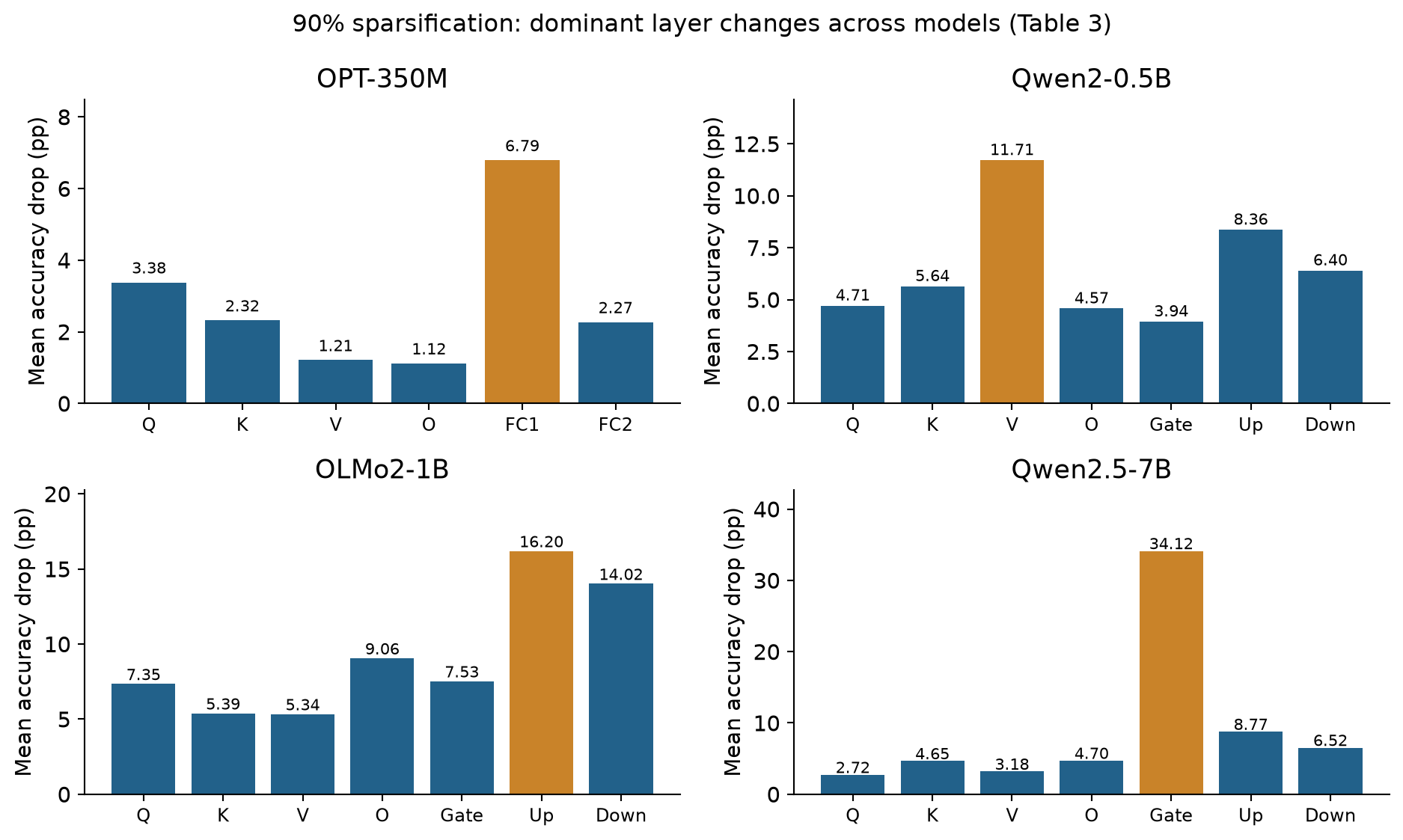
The detailed tasks matter too. Qwen2.5-7B gate sparsification gives drops of 49.16 points on HellaSwag and 47.01 on ARC-Easy, but 21.70 on WinoGrande. The average is useful for scanning, but it hides large task differences. A deployment target with a different task mixture could favor a different compression allocation.

Some OPT entries are negative, such as its Q-row ARC-Challenge change of -1.45 points. Those are reported small improvements on individual tasks, not evidence that sparsification is reliably beneficial. Without uncertainty over seeds or evaluation variation, the sign of a small difference should not bear a broad claim.

The appendix is compatible with heterogeneous, context-dependent sensitivity. It does not support the strongest wording that value projections are always the most vulnerable component. The main normalized perplexity experiment and the appendix raw accuracy experiment differ in sparsity, metric, and normalization, so the distinction is not necessarily a numerical contradiction. It is a limit on transfer of the ranking.

I would preserve that distinction even if all figures looked qualitatively persuasive. A useful compression diagnostic should state its conditioning variables: model family, layer group, perturbation operator, perturbation strength, calibration distribution, and target metric. “V is important” is a good initial hypothesis, not a replacement for those conditions.

9. Limitations and failure boundaries

The most immediate limitation is the proxy chain. We move from a true loss Hessian to a sample gradient second moment, then to a truncated rearranged representation, then sometimes to averaged heatmap pixels. Each step answers a weaker question. Validation of the last picture does not retrospectively establish every earlier equivalence.

The second boundary is finite corruption. A local quadratic can be informative around a reference checkpoint and fail for aggressive uniform quantization or high sparsity. The O-projection discrepancy is valuable evidence of this boundary. It should motivate measuring prediction error as perturbation size grows, rather than removing the inconvenient cases from the summary.

Third, the visual summary and the representation depend on parameter organization. Group sizes, reshaping, signed averaging, and whether attention projections are merged affect the image. A robust policy should be tested against reasonable reorderings and should use an explicitly defined score, not visual brightness alone.

Fourth, the paper gives limited numerical uncertainty. “Strong correlation” is supported largely through qualitative correspondence and selected experimental comparisons. The reviewed tables do not supply a broad held-out rank-correlation study with confidence intervals across calibration draws. A diagnostic can look compelling on several plots yet misorder the marginal cases where allocation decisions are hardest.

Fifth, several protocol details are underspecified for strong budget claims: gradient reduction and caching conventions, sequence length in the timing setup, solver tolerances, exact sparsification rule, and the full repair training budget. I do not fill these gaps from guesses. The reported results remain useful, but comparisons should be bounded by the information actually provided.

Finally, a compact approximation is not automatically positive semidefinite after truncation and diagonal correction. Generic truncated-SVD factors are unconstrained. Even replacing the diagonal of a positive-semidefinite candidate can destroy that property: changing the diagonal of $\begin{pmatrix}2&1.5\\1.5&2\end{pmatrix}$ to $(1,1)$ yields eigenvalues $2.5$ and $-0.5$. This is a general counterexample to an automatic guarantee, not evidence that a reported paper run produced that matrix. Any optimizer that requires a nonnegative curvature penalty must check or enforce the property.

10. Critical analysis: test the interaction in the right coordinates

10.1 A positive perplexity residual does not isolate loss interaction

Let baseline mean negative log likelihood be $\ell_0$ and baseline perplexity be $p_0=e^{\ell_0}$. Suppose two corruptions increase NLL by $a$ and $b$, and suppose their joint NLL increase is exactly $a+b$. This is a case with zero interaction on the NLL scale. Nevertheless,

$$\begin{aligned} D_{\mathrm{PPL}} &=p_0(e^{a+b}-1)-p_0(e^a-1)-p_0(e^b-1)\\ &=p_0(e^{a+b}-e^a-e^b+1)\\ &=p_0(e^a-1)(e^b-1). \end{aligned} \tag{24}$$

If both changes increase NLL, this quantity is positive. With $p_0=10$, $a=0.1$, and $b=0.2$, it is about $0.233$, despite exact additivity in NLL. The same issue is not specific to neural networks: it follows from applying an exponential to an additive variable.

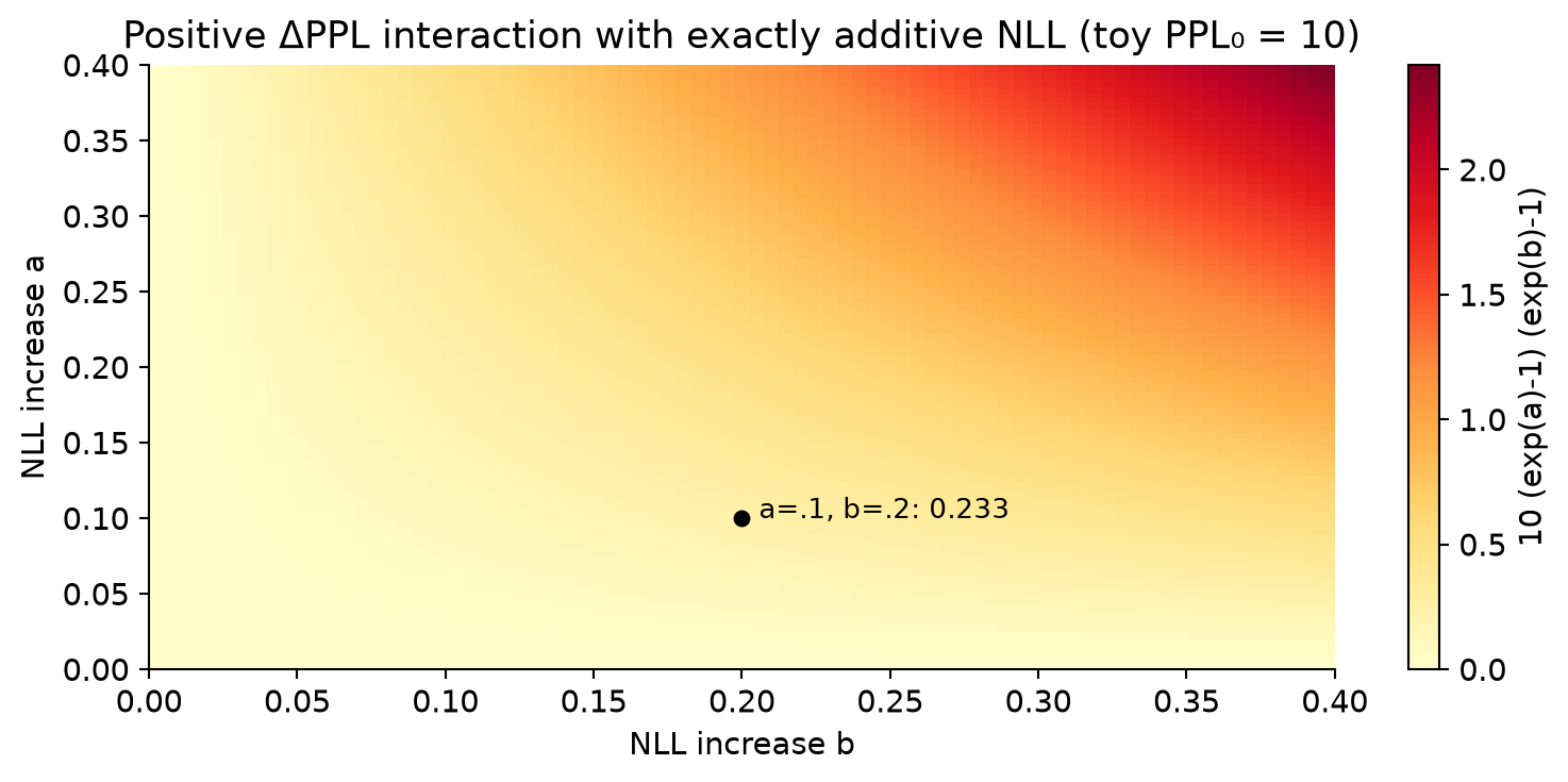
This does not invalidate the observation that a joint corrupted model has greater perplexity than either singly corrupted model. It does weaken the inference that subtracting raw perplexity increases by itself rules out independent loss effects or isolates cross-Hessian coupling. Some part of the residual can arise from the measurement scale.

A directly comparable quantity for a token-averaged NLL Hessian is

$$D_{\mathrm{NLL}} =\log p_{PQ}-\log p_P-\log p_Q+\log p_0. \tag{25}$$

For small, fixed perturbations, the quadratic expansion predicts $D_{\mathrm{NLL}}\approx\delta_P^\top H_{PQ}\delta_Q$, with higher-order corrections. It is important to use the same evaluation tokens and averaging conventions in all four terms. Taking the logarithm of an already averaged collection of sequence perplexities need not recover the intended token-averaged loss.

I would recompute this quantity before claiming a direct causal link between the reported residual and off-diagonal curvature. Appendix B gives changes in perplexity, but not a complete baseline-perplexity table alongside those cells. Without $p_0$ for each exact setup, the displayed differences alone do not allow me to reconstruct every NLL interaction reliably. I therefore leave that numerical question open instead of inventing baselines.

10.2 Test directions, not only blocks

A cross block $H_{PQ}$ can be large while its contraction with a particular error pair is small. Uniform quantization, magnitude sparsification, and low-rank truncation produce different directions. The natural next test is to obtain candidate perturbations, score the signed contraction, and compare it with the measured NLL interaction.

A controlled strength sweep is especially informative. Fix directions $u$ and $v$, apply $\delta_P=t u$ and $\delta_Q=t v$, and measure

$$D_{\mathrm{NLL}}(t) =t^2u^\top H_{PQ}v+O(t^3). \tag{26}$$

Dividing by $t^2$ should approach a stable value within the valid local regime. Failure only at large $t$ points toward nonlocal corruption; failure even at small $t$ implicates the curvature proxy, calibration, or representation. This separates two limitations that the existing plots partly combine.

Such a study should include negative and near-zero predicted interactions, not just the brightest positive pairs. A tool is most useful when it also identifies safe combinations and when its uncertainty prevents an overconfident choice.

10.3 Compare against the cheaper decision rules

The method’s value should be assessed under a fixed preparation budget. Useful controls include diagonal sensitivity, layerwise block approximations, parameter count, activation scale, a small direct corruption sweep, and combinations of these. The relevant outcome is the quality of the chosen compressed model, not just the aesthetic detail of the curvature plot.

For example, a fixed calibration budget could be spent either on more Kronecker terms or on measuring more candidate pair corruptions directly. The better choice depends on how many future configurations will reuse the statistic. An expensive representation may be worthwhile if it guides many compression or repair decisions, yet lose for a one-off compression request.

The paper’s small-network rank sweep and large-model rank-one timings are useful endpoints. A decision-quality-versus-cost curve between them would make the method substantially easier to judge. That curve should include memory, calibration passes, solver time, and the final compression quality at the same retained resource budget.

10.4 Make repair selection compete under equal opportunity

The Schur-complement calculation in Section 7 suggests a more precise repair objective than cross-block magnitude. Estimate recoverable damage while controlling trainable parameters, rank, tokens, and optimization steps. Compare a coupling-informed choice with a value-only heuristic and with a small validation sweep.

For LoRA, equal rank need not mean equal trainable capacity when matrix dimensions differ: a rank-$r$ update has $r(n+m)$ parameters. A policy that always chooses a larger matrix could gain merely from capacity. Conversely, a compact value projection might provide excellent recovery per trainable parameter. Both possibilities deserve an explicit report.

The proposed outlier explanation also admits a useful intervention. Apply a suitable outlier-mitigation transformation, verify its effect on channel statistics, then repeat directional NLL measurements and repair comparisons. A reduction in the targeted interactions would support the mechanism. A quality gain alone would not distinguish outlier mediation from a general change in quantization difficulty.

These are proposed extensions. The checks performed for this review concern algebra, arithmetic, sources, and document rendering; no new model training or compression benchmark is reported.

11. Conclusion

The paper provides a tractable route from whole-group gradient information to a representation that retains cross-layer structure. Rearrangement makes a short Kronecker expansion possible, matrix-free products avoid constructing the giant matrix, and a separately stored diagonal improves the reported small-network fit.

The most useful practical lesson is conditional: compression damage and recovery can depend on relationships between groups, so a purely independent ranking can miss opportunities and failure cases. The experiments make that lesson concrete, particularly through joint corruption and value-projection repair.

The stronger claims need additional care. Empirical Fisher is a proxy, the term count is not an ordinary Fisher rank, linear memory has large constants, and sensitivity rankings change across protocols. Most importantly, a positive residual in perplexity is not sufficient to isolate an interaction in NLL. I would build on this work by testing signed perturbation directions and decision quality under equal preparation and repair budgets.

References and resources

1. Yusupov, V., Cherniuk, D., and Frolov, E. Scalable Kronecker-Fisher Approximation: Efficient Hessian Analysis for Billion-Parameter Language Models Compression, 2026. Main source: Sections 3-5, Tables 1-3, Figures 2-11, Appendices A-C.
2. Full-text HTML of the reviewed version. Formula and table readings were checked against the PDF.
3. No official code resource was identified for this paper in the reviewed arXiv entry or text. The related GFWSVD repository should not be treated as this paper’s resource.