FACTS and CoRS: Which Curvature Should Low-Rank Compression Preserve?

Review date: September 25, 2026
Author: Zhongzhu Zhou
Paper reviewed: Mind the Approximation: Fisher-Weighted SVD Compression for ViTs
Paper authors: Moritz Thoma, Maximilian Groezinger, Maximilian Forstenhäusler, Emad Aghajanzadeh, Ryan Pegoud, Manoj Rohit Vemparala, Pierpaolo Mori, Alexander Frickenstein, Daniel Mueller-Gritschneder, Ulf Schlichtmann
arXiv: 2609.07155v1, submitted September 7, 2026

1. The question that makes this paper worth reading

I usually expect a better approximation to an optimization objective to produce a better decision. FACTS is a useful reminder to ask whether the objective itself is the right one. The paper studies post-training low-rank compression of vision models. Its central observation is that a Kronecker approximation that resembles the empirical Fisher information matrix more closely can preserve less classification accuracy after SVD compression.

The claim is specific. It does not establish that Fisher information is useless, that correlations should always be removed, or that low-rank compression is universally better than pruning. It concerns a particular decision: replacing a shared linear weight with two smaller dense matrices, under a finite compression budget, using curvature statistics collected from a finite calibration set.

Two components address different parts of this decision. FACTS changes the geometry in which a layer is approximated. It suppresses cross-token mixed terms and weights activation statistics by gradient energy, and gradient statistics by activation energy. CoRS, or Constrained Rank Search, chooses a rank for each layer. It measures how compressing one layer changes the full model output, interpolates these measurements, and solves a discrete budget-allocation problem.

This separation matters when reading the headline results. In paper Table 1, Swin-B improves from 60.1% with the strongest listed uniform SVD baselines to 65.9% with uniform FACTS. Adding CoRS reaches 74.9%. These are a 5.8 percentage-point decomposition gain and a further 9.0-point allocation gain. The combined gain over 60.1% is 14.8 points. These three quantities should not be interchanged.

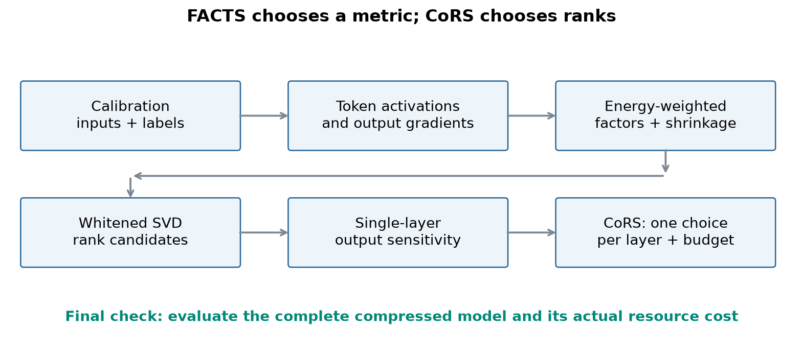
The review proceeds from linear algebra to the estimator, then to allocation and evidence. All experimental numbers below are reported by the authors. Small matrix examples are my explanatory calculations, not model experiments. The source is the complete v1 paper, including Appendices A–C; its protocol details are essential to interpreting the tables.

2. Prerequisites: what low rank actually saves

2.1 A rank is a width, not a percentage of weights

Let a layer apply $W\in\mathbb R^{m\times n}$ to an input $x\in\mathbb R^n$. A rank-$k$ approximation can be represented as $UV$, where $U\in\mathbb R^{m\times k}$ and $V\in\mathbb R^{k\times n}$. The inference path becomes $x\mapsto Vx\mapsto U(Vx)$. No activation is inserted between these two operations: adding one would change the represented linear function.

Ignoring biases, the original layer has $mn$ parameters and the factorized layer has $k(m+n)$. Compression therefore requires

$$k(m+n)<mn, \qquad k<\frac{mn}{m+n}. \tag{1}$$

For a square $768\times768$ matrix, a rank of 384 merely breaks even in parameter count. Retaining half the original linear-layer parameters requires rank 192, not 384. For a rectangular $3072\times768$ MLP matrix, the break-even rank is 614.4. A single rank fraction cannot be interpreted as a uniform parameter fraction across shapes.

For $T$ input tokens, dense arithmetic scales approximately as $Tmn$ multiply-accumulate operations, versus $Tk(m+n)$ after factorization. Counting a multiply and an addition as two FLOPs changes both sides by the same factor. Biases, attention products, normalization, convolution, and other layers remain. A statement about 50% of the compressed linear-layer FLOPs consequently says less than a statement about 50% of the whole model’s work.

2.2 Why ordinary truncated SVD may preserve the wrong directions

Write $W=U_W\Sigma V_W^\top$, with decreasing singular values. Ordinary truncated SVD solves

$$\min_{\operatorname{rank}(\widetilde W)\le k} \|W-\widetilde W\|_F^2 =\sum_{j>k}\sigma_j^2. \tag{2}$$

This is an exact statement about squared weight error. The model does not directly evaluate that norm. It evaluates predictions on a distribution of inputs. If an input direction almost never occurs, accurately preserving its corresponding weight direction may have little practical value. If an output direction changes the decision boundary, a small weight error there may matter greatly.

An activation-aware objective introduces $A=\mathbb E[xx^\top]$:

$$\mathbb E\|(W-\widetilde W)x\|_2^2 =\operatorname{tr}\bigl((W-\widetilde W)A(W-\widetilde W)^\top\bigr). \tag{3}$$

The right-hand metric asks which inputs occur. A left-hand metric $B$ additionally distinguishes sensitive output directions. FACTS uses both. This is why its SVD is performed on a transformed weight, not directly on $W$.

2.3 Curvature is a local surrogate

For a perturbation $\delta\theta$, the Taylor expansion is

$$\Delta\mathcal L\approx \nabla\mathcal L^\top\delta\theta +\frac12\delta\theta^\top H\delta\theta. \tag{4}$$

Dropping the linear term presumes an appropriate stationary-point approximation. Replacing the Hessian with Fisher information needs additional modeling assumptions. The empirical Fisher formed with observed labels is not automatically equal to the true expected Hessian of an arbitrary trained model. Appendix C states an expected-Hessian/Fisher relation under regularity conditions, together with layer-block and positive-definiteness assumptions. Those assumptions define the scope of the optimality argument.

Low-rank removal can also be a large perturbation. A perfect quadratic approximation near the original weight need not predict the final model after many layers are compressed. I therefore interpret Fisher weighting as a useful local design choice, whose final value must be checked on the actual prediction task.

3. Deriving the weighted SVD solution

3.1 From a huge Fisher matrix to two manageable factors

For column-wise vectorization of a matrix perturbation $D=W-\widetilde W$, the per-layer Fisher has shape $mn\times mn$. Even a $768\times768$ layer would have a curvature matrix with roughly 348 billion entries. A single Kronecker approximation replaces it with

$$F\approx A\otimes B, \qquad A\in\mathbb R^{n\times n},\quad B\in\mathbb R^{m\times m}. \tag{5}$$

The storage reduction is from order $m^2n^2$ to $m^2+n^2$. This is substantial, but dense factors and their decompositions can still be expensive for wide layers. FACTS avoids constructing the full Fisher; it does not make calibration free.

The vectorization identity gives a directly interpretable matrix objective:

$$\begin{aligned} \operatorname{vec}(D)^\top(A\otimes B)\operatorname{vec}(D) &=\operatorname{tr}(D^\top BDA)\\ &=\|B^{1/2}DA^{1/2}\|_F^2. \end{aligned} \tag{6}$$

Here I use symmetric positive-definite square roots to remove ambiguity about triangular-factor conventions. Define $Z=B^{1/2}WA^{1/2}$. Invertibility preserves rank, so minimizing the weighted error over rank-$k$ weights is equivalent to approximating $Z$ in ordinary Frobenius norm. If $Z_k=U_k\Sigma_kV_k^\top$, the solution is

$$\widetilde W_k=B^{-1/2}U_k\Sigma_kV_k^\top A^{-1/2}. \tag{7}$$

One convenient split for inference is

$$W_{\rm out}=B^{-1/2}U_k\Sigma_k^{1/2}, \qquad W_{\rm in}=\Sigma_k^{1/2}V_k^\top A^{-1/2}. \tag{8}$$

The product equals $\widetilde W_k$. The two factors contain the whitening geometry during construction; inference only needs the final dense matrices. Cholesky is an alternative factorization, but its transposes must agree with the stated convention. Appendix C’s proof provides that convention more explicitly than the compact pseudocode.

3.2 A small example of changing what survives

Consider $W=\operatorname{diag}(4,2)$ and rank one. Ordinary SVD keeps the first coordinate. Now let $A=I$ and $B=\operatorname{diag}(1,9)$. The transformed matrix is $Z=\operatorname{diag}(4,6)$, so weighted SVD keeps the second coordinate instead. Dropping the second coordinate costs $9\cdot2^2=36$ in the weighted objective; dropping the first costs $1\cdot4^2=16$.

The example explains the mechanism without asserting that an actual model has these statistics. “Smaller singular value” is meaningful only after specifying the metric. It also shows why comparing unweighted reconstruction errors alone can favor the wrong compressed model.

A global positive scale on $A\otimes B$ does not change the exact minimizer of this objective. Relative directions and relative eigenvalues do. Numerically, normalization and regularization can still affect the computation, particularly when eigenvalues are nearly zero. A mathematical scale invariance should not be confused with numerical invariance under an arbitrary stabilization rule.

4. Shared weights create two different correlation questions

4.1 Cross-token moments arise before any approximation

At token position $t$, let $x_t$ be the input and $g_t$ the gradient with respect to the layer output. Because the same weight is reused at every position, the per-example weight gradient is a sum:

$$\nabla_W\mathcal L=\sum_{t=1}^T g_tx_t^\top. \tag{9}$$

Taking its outer product introduces every token pair:

$$F=\mathbb E\left[\sum_{t=1}^T\sum_{s=1}^T (x_tx_s^\top)\otimes(g_tg_s^\top)\right]. \tag{10}$$

The diagonal pairs $t=s$ describe within-position sensitivity. Off-diagonal pairs describe how errors at different positions interact. For a chosen perturbation $D$, define $e_t=g_t^\top Dx_t$. Then

$$\mathbb E\left[\left(\sum_t e_t\right)^2\right] =\sum_t\mathbb E[e_t^2] +\sum_{t\ne s}\mathbb E[e_te_s]. \tag{11}$$

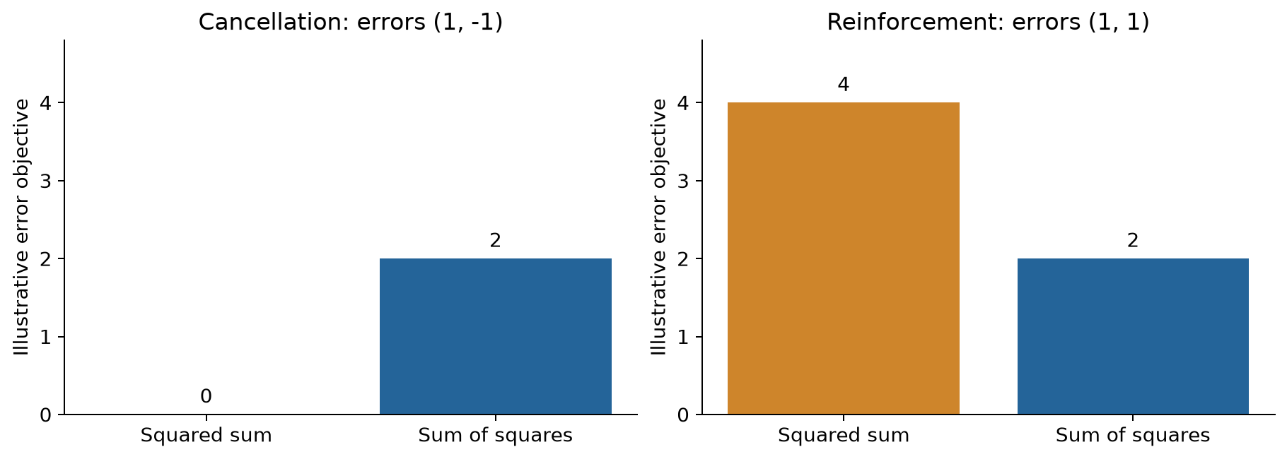
The cross terms may reinforce or cancel. In an illustrative two-token example, errors $(1,-1)$ give zero total squared error but a token-local sum of squares of two. Errors $(1,1)$ give a total of four and the same local sum of two. Removing cross terms changes the objective; it does not simply estimate the same quantity with fewer samples.

Vision tokens often correspond to spatial positions with persistent meaning across images. The paper’s diagnostics show structured cross-token interactions in DeiT, Swin, ConvNeXt, and MambaVision. Yet those structures do not by themselves establish which directions a finite-rank approximation should preserve. A covariance heatmap shows that a relationship exists; it does not show that fitting that relationship improves the downstream decision.

4.2 Token locality and activation–gradient dependence are separate axes

KFAC-expand uses token-local statistics but separates activation and gradient moments. KFAC-reduce aggregates over tokens before forming its factors, while still separating the two kinds of moments. Shampoo2 and GFWSVD target the dominant structure of a global Fisher approximation and can reflect both cross-token structure and activation–gradient dependence.

The paper’s gap in this design space is a token-local estimator that retains some within-token dependence. FACTS fills this gap using energy-weighted moments. This is a more precise description than saying it “keeps all useful correlations.” It neither preserves the entire joint distribution nor proves that every removed correlation is harmful.

The authors report activation–gradient distance correlation, not just ordinary linear correlation. Their cross-token heatmap is a normalized diagnostic based on products of Gram matrices; Appendix A.1 explicitly says it is not itself the Fisher approximation. Maintaining this distinction prevents a visually compelling heatmap from becoming stronger evidence than the underlying experiment provides.

5. FACTS: a token-local curvature construction

5.1 From a global contraction to energy-weighted moments

Stack the token inputs and output gradients as rows of $X\in\mathbb R^{T\times n}$ and $G\in\mathbb R^{T\times m}$. A global contraction from identity initialization contains

$$\begin{aligned} \mathbb E[G^\top XX^\top G] &=\mathbb E\left[\sum_{t,s} (x_t^\top x_s)g_tg_s^\top\right]. \end{aligned} \tag{12}$$

The paper introduces Zero Cross-Moment, or ZCM, as a structural prior: the relevant contracted terms with $t\ne s$ are dropped in expectation. For the right factor this leaves

$$B_0=\mathbb E\sum_t\|x_t\|_2^2g_tg_t^\top =\mathbb E[G^\top\operatorname{diag}(XX^\top)G]. \tag{13}$$

The symmetric token-local contraction gives

$$A_0=\mathbb E\sum_t\|g_t\|_2^2x_tx_t^\top =\mathbb E[X^\top\operatorname{diag}(GG^\top)X]. \tag{14}$$

The resulting approximation is

$$\widehat F_{\rm FACTS}=\frac{A_0\otimes B_0}{c}, \qquad c=\mathbb E\sum_t\|x_t\|_2^2\|g_t\|_2^2. \tag{15}$$

Both factors have trace $c$. Consequently the Kronecker product divided by $c$ also has trace $c$, matching the trace of the token-local sum. This supplies a useful interpretation of the normalization, provided $c>0$. A layer with zero observed gradients requires a separate fallback; dividing by zero is not a meaningful curvature estimate.

The notation $\operatorname{diag}(XX^\top)$ means a diagonal matrix containing row-wise squared norms. It does not require storing the full $T\times T$ matrix. One can compute those norms directly. This observation follows from the formula and explains why token locality can reduce an otherwise unnecessary intermediate; it is not a statement about the authors’ software.

5.2 What dependence is retained?

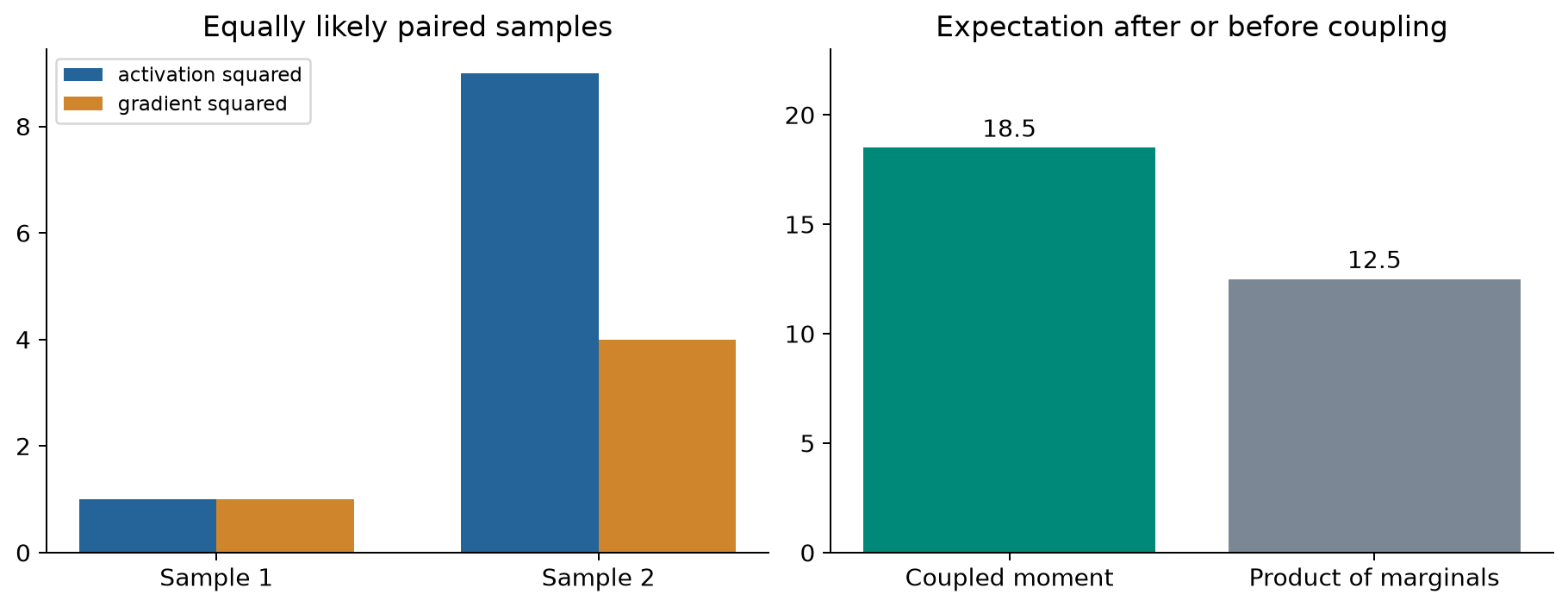
In $A_0$, each activation outer product is weighted by the gradient energy from the same token. In $B_0$, each gradient outer product is weighted by the corresponding activation energy. Taking the expectation after this weighting differs from multiplying separate expectations.

For a scalar illustration, suppose equally likely samples are $(x,g)=(1,1)$ and $(3,2)$. The coupled moment is $\mathbb E[x^2g^2]=(1+36)/2=18.5$. The decoupled product is $\mathbb E[x^2]\mathbb E[g^2]=5\cdot2.5=12.5$. The difference is not an implementation detail: it changes which samples dominate the metric.

There is still an approximation. A single Kronecker product cannot represent every fourth-order interaction. FACTS preserves a particular energy-mediated dependence, not the full joint activation–gradient tensor. Similarly, its one-step construction should not be read as a general guarantee that the best Kronecker product has been found. The later truncated SVD is optimal for the chosen positive-definite metric; choosing that metric is a different problem.

5.3 Regularization changes the metric in a controlled direction

The paper’s pseudocode uses shrinkage of row and column factors, with strengths 0.7 and 0.1, respectively. For a factor $C$ of dimension $d$, this has the form

$$C_\alpha=(1-\alpha)C+\alpha\frac{\operatorname{tr}(C)}{d}I. \tag{16}$$

If $C$ has positive trace and is positive semidefinite, $\alpha>0$ lifts zero eigenvalues. It keeps the same eigenvectors while moving eigenvalues toward their mean. This stabilizes inverse square roots, at the cost of changing the objective. Large shrinkage moves the method toward a less anisotropic metric. The effect is especially relevant when comparing FACTS with a baseline whose factors become ill-conditioned.

Algorithm 1: FACTS compression, mathematical workflow. This numbered description reorganizes paper Algorithms 1–2 while making factor orientation explicit.

1. Fix a pretrained model, calibration examples and labels, eligible linear layers, and a target rank for each layer. Keep the classification head outside the compressed set, as in the main experiments.
2. For each calibration batch, perform a forward pass and a cross-entropy backward pass. Collect $x_t$ and $g_t$ at each eligible layer; apply the stated gradient stabilization.
3. Accumulate the token-local energy-weighted moments in Equations 13–14, retaining consistent sample normalization. Compute the positive trace normalization when defined.
4. Associate the column factor with $A$ and the row factor with $B$. Apply shrinkage, and explicitly choose a square-root or Cholesky convention.
5. Form $Z=B^{1/2}WA^{1/2}$, then compute its SVD and retain the requested $k$ singular components.
6. Form the two unwhitened factors in Equation 8. Retain any original bias at the output of the pair.
7. Replace the eligible map with these consecutive linear maps. Evaluate the jointly compressed model using held-out predictions and the actual resource budget.

The failure boundaries are concrete: a poorly matched calibration set weights the wrong inputs; extreme rank removal exceeds the local approximation; singular factors make unwhitening unstable; and errors from many layers may interact. Regularization mitigates one of these problems, not all of them.

The same procedure in compact pseudocode, with symmetric square roots:

01 Initialize A0[i], B0[i] = 0 for each eligible layer i
02 For each calibration example:
03   Run forward and backward to obtain token pairs (x, g)
04   For each eligible layer i and token t:
05     A0[i] += norm(g[t])^2 * outer(x[t], x[t])
06     B0[i] += norm(x[t])^2 * outer(g[t], g[t])
07 For each eligible layer i:
08   Normalize moments; handle zero trace; apply shrinkage
09   Z = sqrt(B[i]) * W[i] * sqrt(A[i])
10   U, S, Vt = truncated_SVD(Z, rank[i])
11   Left  = invsqrt(B[i]) * U * sqrt(S)
12   Right = sqrt(S) * Vt * invsqrt(A[i])
13   Replace W[i] by Left * Right, retaining output bias

6. CoRS: allocate a budget across unequal layers

6.1 Measure the effect at the model output

For every layer $i$ and candidate rank $j$, CoRS measures an error $e_{ij}$ after compressing only that layer. In the classification setup this is a KL-divergence measurement between the original model output and the perturbed model output, on 512 calibration images. It pairs this with cost $f_{ij}$. Measuring the final output makes the scores more comparable across layers than raw singular-value energy.

The original layer is an explicit candidate with zero error. This is essential. Without it, a solver could be forced to compress an unusually sensitive layer even when leaving it dense would be the best use of the budget. The main setup profiles five remaining-cost ratios, 0.1, 0.3, 0.5, 0.7, and 0.9, and interpolates a denser set between them.

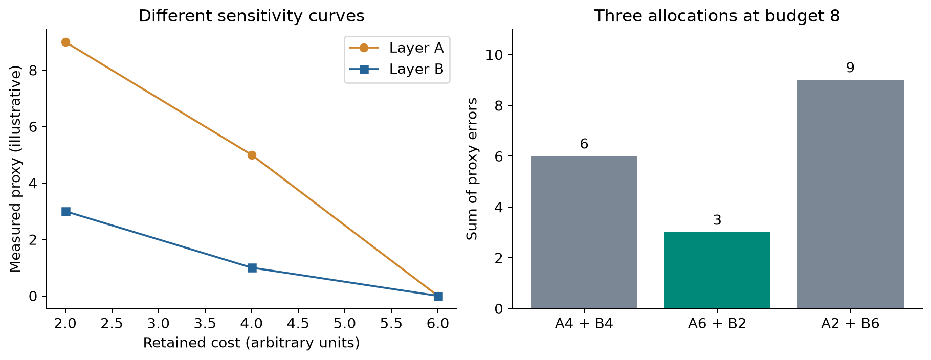
For intuition, imagine two layers with choices costing two, four, or six units. Layer A’s errors are 9, 2, and 0; layer B’s are 3, 1, and 0. Under an eight-unit budget, uniform allocation costs four units per layer and has proxy error three. Giving six units to A and two to B also costs eight and has error three. In a slightly more sensitive A, with middle error five, uniform error rises to six while the asymmetric choice stays at three. The best allocation depends on the shape of both curves, not just their uncompressed size.

6.2 The discrete optimization and what its guarantee means

Introduce $z_{ij}\in\{0,1\}$, selecting one configuration per layer:

$$\begin{aligned} \min_z\quad &\sum_i\sum_j e_{ij}z_{ij}\\ \text{subject to}\quad &\sum_i\sum_j f_{ij}z_{ij}\le B_{\rm FLOPs},\\ &\sum_jz_{ij}=1\quad\text{for every }i. \end{aligned} \tag{17}$$

This is a multiple-choice discrete budget problem expressed as a mixed-integer linear program. Its objective and constraints are linear in the binary decisions. A solver that certifies optimality solves this finite proxy problem. It does not certify the best classification accuracy, the best latency, or the best rank choice outside the candidate set.

The additive proxy omits interactions between simultaneously compressed layers. In a second-order view, a joint perturbation includes cross-layer terms of the form $\delta_i^\top H_{ij}\delta_j$. Summing isolated errors cannot recover those terms. CoRS is therefore best understood as a strong, efficiently searchable allocation model whose predictions are subsequently evaluated on the complete compressed network.

6.3 Interpolation is part of the optimization model

A cubic fit can invent a low-error dip between sparse measurements. A solver will exploit that dip even if it has no physical meaning. The paper proposes local cubic fits over overlapping triplets, compared against a piecewise-linear reference, to reduce such artifacts.

Appendix C contains a detail worth preserving: the prose describes selecting a prediction by pointwise deviation, whereas Algorithm 3 scores a whole window by summed absolute deviation. The prose also discusses retaining monotone splines, but the pseudocode does not explicitly show that rejection. These are ambiguities in the written method, not reasons to invent a definitive procedure. The authors themselves report only marginal gains over linear interpolation, which is a sensible alternative for a carefully controlled comparison.

Algorithm 2: CoRS rank allocation, following the paper’s stated stages.

1. Keep the original model as the output reference and fix the set of eligible layers and the total FLOP accounting convention.
2. For each layer, evaluate its five sparse compression candidates in isolation. Store the measured output divergence and the corresponding arithmetic cost.
3. Add the original dense layer with zero proxy error. Construct a denser candidate profile using the specified interpolation variant; record its exact convention.
4. Convert candidate choices into valid integer ranks and their resulting costs. Remove duplicate configurations created by rounding.
5. Solve Equation 17 with the FLOP budget and exactly-one-choice constraint. Record feasibility and the achieved optimization gap rather than assuming every solver termination is a proof of optimality.
6. Materialize all selected factorizations together and measure the complete model. Compare realized quality and cost with the predicted objective.

Steps concerning rank rounding, feasibility reporting, and final joint evaluation make explicit the practical conditions of the mathematical problem. They are requirements for a meaningful assessment, not evidence that a particular software path was exercised. Once the profiles are built, the same profiles can support several budgets; the expensive sensitivity measurements can be amortized.

01 Reference = outputs(original_model, profiling_images)
02 For each eligible layer i:
03   Profile[i] = {(original_cost[i], 0, dense_choice)}
04   For each sparse candidate rank k:
05     Candidate = original_model with only layer i compressed
06     e = output_divergence(Reference, outputs(Candidate))
07     Add (actual_cost(i, k), e, k) to Profile[i]
08   Interpolate Profile[i]; round ranks; merge duplicates
09 Solve: minimize selected_error_sum subject to cost <= B
10 Require exactly one choice per layer; report solver gap
11 Evaluate all selected layers together on held-out data

7. Experimental evidence: compare within a protocol

7.1 Does a more accurate Fisher approximation predict accuracy?

Paper Table 2 holds the decomposition pipeline and per-model arithmetic budget fixed while comparing estimators. The following values are direct transcriptions; cosine similarity is to the empirical Fisher, not prediction accuracy.

Estimator	DeiT cosine	DeiT Top-1	Swin cosine	Swin Top-1
GFWSVD	0.174	71.0	0.117	52.2
Shampoo2	0.166	77.2	0.177	75.9
KFAC-reduce	0.129	67.0	0.138	56.5
KFAC-expand	0.119	75.9	0.103	75.3
FACTS	0.128	77.5	0.127	76.6

The budgets are 17.1 GFLOPs for DeiT-B and 18.4 GFLOPs for Swin-B. They are matched within each column group, not across the two models. FACTS improves on Shampoo2 by 0.3 and 0.7 points. These modest gaps support the estimator choice, but the much larger gaps to ill-conditioned baselines mix structural modeling and numerical stability.

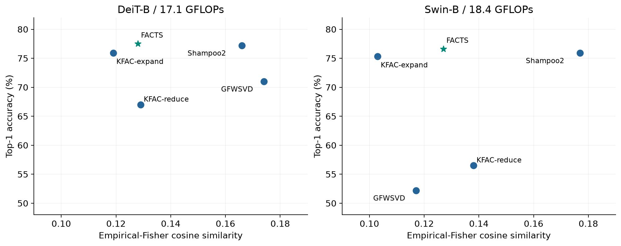
Appendix A.1 estimates the operator cosine using random probe matrices and Fisher-vector products. This avoids forming the full matrix. It uses 16,000 class-balanced validation images for the diagnostic factors and a disjoint 2,000-image set for the cosine and qualitative diagnostics. The main decomposition protocol instead specifies 16,384 images from the training set. Those protocols should not be silently merged into a single calibration description.

The GFWSVD adaptation uses 64-sample averaged gradients because of memory constraints; the paper identifies conditioning as a practical failure mode. This is important context for its poor scores. The results demonstrate an advantage under the paper’s stated vision adaptation. They do not establish that all possible implementations or calibration choices of GFWSVD necessarily fail.

7.2 Separate decomposition gains from allocation gains

At 50% of the eligible linear-layer FLOPs remaining, Table 1 reports:

Model	Full model	FLAR-SVD	FACTS uniform	FACTS + CoRS
DeiT-B	83.3	75.0	77.5	81.3
Swin-B	85.1	60.1	65.9	74.9
ConvNeXt-B	85.8	72.2	75.8	79.4
MambaVision-B	83.9	71.3	72.3	79.7

All entries are Top-1 percentages. The compressed whole-model costs are 17.1, 15.5, 15.9, and 21.5 GFLOPs, respectively. MambaVision’s full model is 29.9 GFLOPs, so its whole-model saving is only about 28.1%, despite the 50% eligible-linear-layer target. This is a useful example of why the compressed component and the complete network need separate denominators.

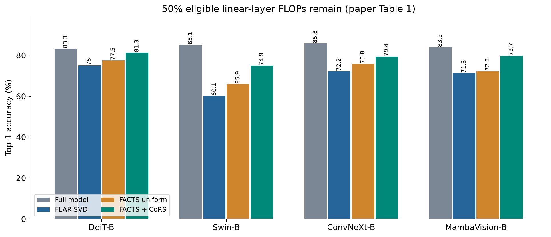
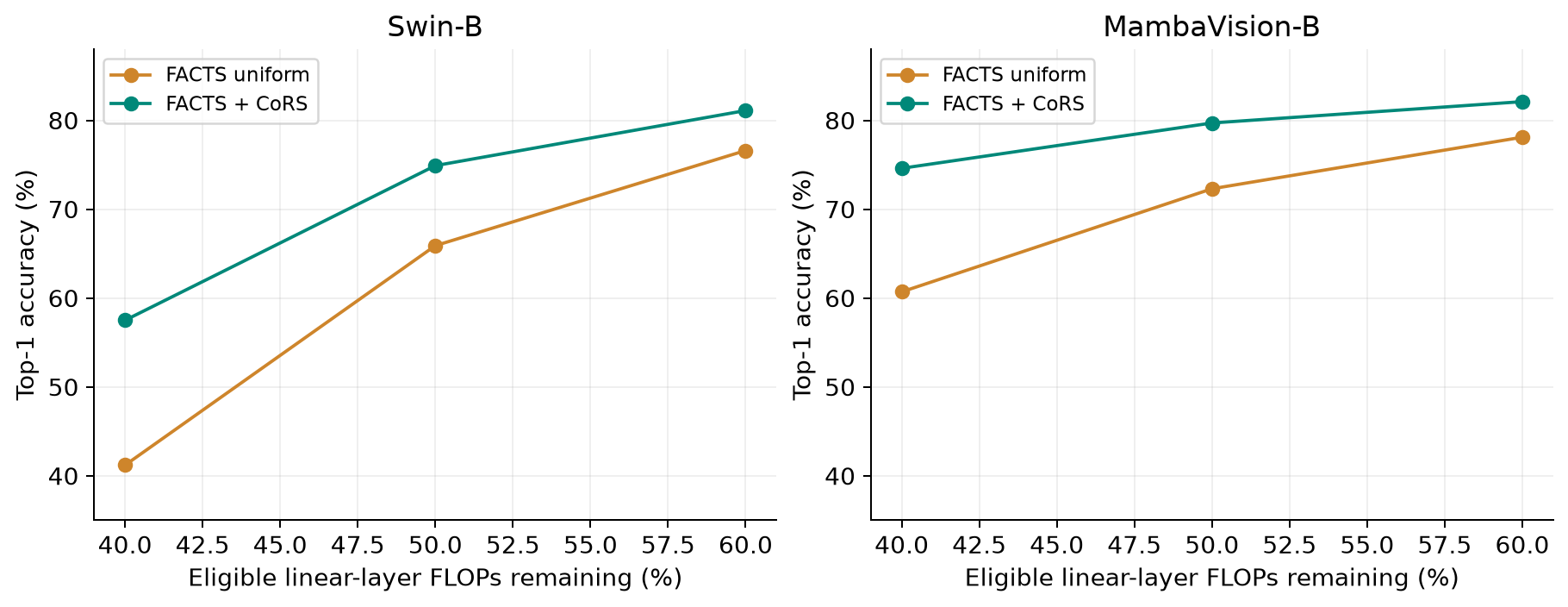
The allocation gain is especially large on architectures for which uniform compression is destructive. At the more aggressive 40% remaining-linear-FLOP target, paper Table 8 gives Swin-B 41.2% with uniform FACTS and 57.5% with CoRS. MambaVision rises from 60.7% to 74.6%. These results suggest strong layer heterogeneity, but they also show that a favorable comparison with other compressed models can coexist with substantial degradation from the uncompressed model.

7.3 Search time is not just solver time

Table 3 compares allocation strategies while using FACTS as the underlying decomposition. CoRS reaches 79.8% in 6.6 minutes for DeiT-B and 81.3% in 15.0 minutes for Swin-B. MemViT is far faster at 0.1 minutes but reaches 78.1% and 79.0%. ASVD search reaches 79.1% in 19.9 minutes and 80.2% in 26.5 minutes. The paper describes the MILP solve itself as taking only seconds; the full search times also reflect profiling.

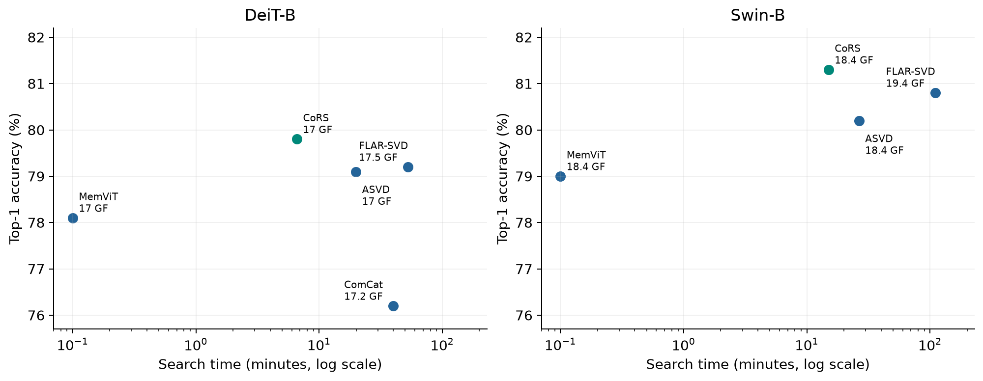
FLAR-SVD in that table reaches 79.2% at 17.5 GFLOPs for DeiT-B and 80.8% at 19.4 GFLOPs for Swin-B. CoRS uses 17.0 and 18.4 GFLOPs. CoRS therefore wins this reported comparison despite a smaller arithmetic budget, but calling every entry exactly budget-matched would be inaccurate.

The DeiT baseline in Table 3 is 81.8%, while Table 1 uses 83.3%. Its uniform row also differs. I compare methods within the same table and do not combine those rows into a single controlled ablation. Appendix Table 12 supplies another useful decomposition/search timing breakdown, but likewise contains baseline and ratio labels that require careful interpretation.

7.4 Throughput is encouraging, with a narrower claim than FLOPs

Paper Figure 2 labels DeiT-B throughput speedups of 1.6× on V100, 1.7× on A100, 1.6× on H100, and 1.6× on the tested Intel Xeon CPU. Those reported factors are redrawn below; I do not infer exact images-per-second values from bar heights.

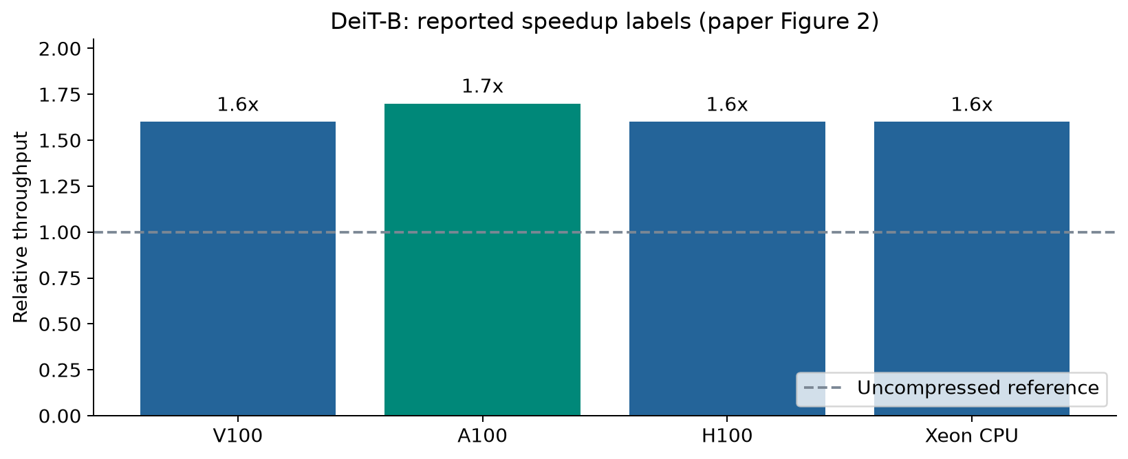
The mechanism is plausible: two smaller dense matrix multiplications can use ordinary dense kernels without sparse indexing. But adding a matrix multiplication also adds scheduling and intermediate-memory costs. The speedup depends on matrix shapes, batch size, precision, software stack, and the rest of the network. The paper’s semi-structured-pruning comparison should consequently be read as a measurement of its chosen deployment path, not a universal verdict on hardware sparsity.

An elementary accounting model helps. Let $p$ be the fraction of latency attributable to the compressed operations, $r$ their cost fraction after compression, and $h$ added overhead measured relative to original total latency. Then an illustrative idealized speedup is

$$S\approx\frac{1}{(1-p)+pr+h}. \tag{18}$$

With $p=0.8$, $r=0.5$, and $h=0$, the model gives 1.67×. This is an explanatory estimate, not a fit to the reported measurements. It shows why halving eligible arithmetic does not imply doubling end-to-end throughput.

8. Transfer results, calibration, and a restrained LLM reading

The downstream evidence is useful because it tests more than ImageNet classification. Paper Table 6 compares compressed Swin-B backbones in Mask R-CNN on COCO. At 290.3 GFLOPs, FACTS reaches box mAP 45.3 and mask mAP 41.6, versus 42.9 and 39.5 for SVD-LLM. The uncompressed model gives 46.6 and 42.6 at 358.5 GFLOPs. One epoch of fine-tuning raises FACTS to 45.9 and 42.1.

PELA reaches box mAP 45.3 and mask mAP 41.3, but follows a different multi-stage retraining protocol. That makes it relevant as a quality/effort comparison, not an isolated comparison of the same training recipe. The paper’s zero-shot compression is applied to an already converged downstream model; it does not mean the downstream task was never trained. Appendix A.5 also changes sensitivity measurement for detection to an FPN feature-map MSE, using ten images. The method’s reusable idea is output-aware profiling; KL on classifier probabilities is one instantiation.

On ADE20K in Table 7, DeiT-B FACTS reaches 43.5 mIoU, versus 38.1 for SVD-LLM and 44.9 for the full model. Swin-B FACTS reaches 46.2, versus 37.7 and 49.4. The full-system GFLOP reductions are much smaller than 50%: only the backbone is compressed and task-specific heads remain. These results again reward precise accounting.

Calibration is not a minor footnote. The primary decomposition setup uses 16,384 images and backward passes. Table 10 shows that FACTS without search is not uniformly best at small sample counts: with 1,024 images, DeiT-B FACTS scores 73.7 while FLAR-SVD scores 74.4; MambaVision FACTS scores 71.8 while GFWSVD scores 77.8. Adding CoRS improves the overall result, but this should not erase the estimator’s sensitivity to calibration data.

The LLM experiment is explicitly exploratory. Qwen3-1.7B is compressed uniformly to 0.7 remaining parameters, calibrated on 256 WikiText2 training sequences of length 2,048. Table 11 reports:

Method	WikiText perplexity ↓	Mean zero-shot accuracy ↑
SVD-LLM	57.7	35.4
GFWSVD	>1,000	31.3
Shampoo2	44.6	34.4
FACTS	40.8	36.5

Relative to Shampoo2, perplexity falls by about 8.5%, calculated as $(44.6-40.8)/44.6$. Accuracy rises by 2.1 points. The result is interesting, but one small LLM and one calibration setting cannot establish broad robustness on long context, reasoning, instruction following, or large language models. The table also does not provide an uncompressed row, so I do not invent one or report a recovery fraction.

9. Limitations and failure boundaries

The most direct limitation is objective mismatch. FACTS deliberately changes the Fisher approximation using a token-local prior. Its empirical success is evidence for that choice in the tested settings; it is not proof that true cross-token interactions vanish. Tasks with useful cancellation, unusual token aggregation, or different spatial statistics may prefer another prior.

A second limitation is the finite calibration distribution. Energy weighting can amplify rare high-gradient or high-activation samples. Gradient stabilization and shrinkage help, but their interaction with class imbalance, domain shift, and calibration size remains important. A strong result on ImageNet-based calibration does not automatically predict behavior on medical images, unusual resolutions, or strongly shifted deployment data.

Third, layerwise curvature and rank allocation both simplify interactions. The second-order derivation treats layer blocks separately. CoRS adds isolated-layer output divergences. Compressing an early layer changes the inputs received by later layers, so both their metric and their sensitivity profile may change in the joint model. This is particularly relevant at aggressive budgets.

Fourth, some reported improvements are small enough that uncertainty matters. The reviewed tables generally provide point estimates rather than confidence intervals or repeated-calibration distributions. A 0.3-point advantage over Shampoo2 is not as conclusive as a much larger, repeated separation would be. The paper’s broad architectural coverage is valuable, but breadth does not substitute for uncertainty estimates.

Finally, the method has a preparation cost. Collecting gradients, factoring dense statistics, and profiling each layer consumes resources before inference savings begin. For a model served many times this can be reasonable. For frequent model updates, tiny deployment workloads, or restricted access to calibration labels, a cheaper approximation may be preferable even with somewhat lower accuracy.

10. Critical analysis: what I would resolve next

10.1 Distinguish three kinds of optimality

The most important conceptual correction is to keep three claims separate. Truncated SVD is optimal for a fixed positive-definite weighted Frobenius objective. A one-step energy-weighted construction is a way to choose the Kronecker metric; it is not generally the converged best rank-one approximation of the rearranged Fisher. A certified MILP solution is optimal for a finite additive profile; it is not optimal for the real network’s accuracy.

This distinction strengthens the paper’s practical contribution. The compelling idea is to design a useful compression surrogate, rather than optimize Fisher reconstruction as an end in itself. I would test that idea directly by measuring whether each surrogate ranks a common set of actual compression perturbations correctly. Operator cosine measures average matrix alignment; rank correlation between predicted damage and realized damage addresses the decision the method must make.

10.2 Isolate structural benefit from stabilization benefit

Table 2 combines meaningful structural comparisons with severe numerical failures. A cleaner study would compare token-local and global estimators at matched calibration samples, gradient treatment, and shrinkage grids. It would report factor condition numbers and held-out compressed-model quality alongside the Fisher cosine. If FACTS remains better after these conditions are aligned, the argument for its structural prior becomes stronger.

A particularly useful ablation would interpolate between token-local and cross-token objectives with a coefficient selected on held-out calibration data. Such a study could reveal when discarding mixed terms is beneficial, instead of treating locality as a universal binary choice. This is a proposed experiment, not a result of the paper or this review.

10.3 Reconcile the tables before turning them into deployment promises

The main paper mixes DeiT baselines of 83.3 and 81.8 across tables. Table 4 reports FACTS after one epoch at 81.4 against a displayed baseline of 83.3, a 1.9-point gap. The nearby prose calls it within 0.4 points, which would instead match the 81.8 baseline used elsewhere. I cannot resolve that discrepancy from the printed evidence, so I retain the table values and avoid the near-baseline claim.

Similarly, Table 12’s Swin uniform accuracy of 76.6 matches the 60%-remaining result elsewhere, even though its caption says compressed to 50%. Table 3’s FLAR-SVD budgets differ from CoRS. None of these observations negates the within-table comparisons, but they obstruct a single clean causal story. A unified table with exact checkpoint identifiers, input resolution, budget denominator, fine-tuning schedule, and separate decomposition/profiling/solver times would make the results substantially easier to evaluate.

10.4 Give the optimizer better evidence at the points it chooses

A practical improvement to CoRS is adaptive remeasurement. After an initial solve, measure the selected interpolated ranks directly. If their errors disagree with the interpolation, update the profiles and solve again. Then evaluate a small number of jointly compressed layer pairs that appear especially sensitive. This focuses expensive measurements on decisions the optimizer actually uses.

For latency-sensitive deployment, the same framework could use measured per-configuration latency in place of FLOPs, with a final whole-model latency check. However, per-layer latencies may also fail to add because of fusion, memory traffic and parallel execution. Changing the cost column is a useful starting point, not an automatic latency guarantee.

11. A paper-based evaluation plan

For a future experimental study, I would first fix one model, one eligible-layer set, and one unambiguous budget. I would separate three data roles: factor calibration, rank-profile selection, and final evaluation. The diagnostic validation split from Appendix A.1 should remain distinct from a final reported test set.

Next I would compare ordinary SVD, activation-aware SVD, KFAC-expand, Shampoo2, and FACTS under uniform compression. This isolates decomposition. Only then would I hold the decomposition fixed and compare uniform ranks, a simple greedy rule, linear-interpolated CoRS, and the paper’s local-cubic version. Rounding and the dense-layer option must be identical across allocation comparisons.

The report should include accuracy with multiple calibration draws, whole-model parameters and FLOPs, factor-statistics cost, profile cost, solver time, and real end-to-end throughput. For the algebra, the trace identity, factor shapes, weighted reconstruction objective, and break-even rank can be checked with small matrices. Those checks validate the explanation; they cannot reproduce ImageNet accuracy or GPU speedup.

This review does not report new model training, compressed-model benchmark runs, or replication of the authors’ results. The official resource link is included for future readers, while the technical account here is grounded in the paper and its appendix.

12. Conclusion

FACTS is valuable because it puts the approximation target under scrutiny. It shows that closer empirical-Fisher reconstruction and better finite-rank compression are different objectives. Its token-local, energy-weighted factors offer a practical way to retain useful activation–gradient information without explicitly fitting every cross-token interaction.

CoRS adds a complementary lesson: selecting ranks across heterogeneous layers can matter as much as improving the per-layer decomposition. The strongest reading of the paper is therefore a combination of a purpose-specific metric and a budget-aware search. The boundaries remain clear: local curvature, calibration quality, additive rank profiles, and actual deployment costs all need independent attention.

References and resources

1. Thoma et al. Mind the Approximation: Fisher-Weighted SVD Compression for ViTs, 2026. Main source: Sections 3–6, Tables 1–12, Figures 1–7, Appendices A–C.
2. Official FACTS resource, linked by the arXiv abstract page. Resource entry only.
3. Thoma et al. Advancing SVD-based LLM Compression via Layer-Wise Error Model Search, ICML 2026. Related paper identified by the FACTS bibliography; its full text was unavailable during this reading and is not treated as evidence for additional claims.

Figures 1–4 are original explanatory constructions. Figures 5–8 redraw explicitly cited paper tables; Figure 9 redraws reported relative-speed labels. Equation numbers in this review are local to this review.