Deep Delta Learning: Editing the Residual Stream, and Accounting for the Cost

Review date: September 24, 2026
Author: Zhongzhu Zhou
Paper reviewed: Deep Delta Learning
Paper authors: Yifan Zhang, Yifeng Liu, Mengdi Wang, Quanquan Gu
arXiv: 2601.00417v4, revised July 27, 2026; first submitted January 1, 2026.
this review uses the complete 20-page v4, including Appendices A-D.
Resources: Versioned paper · Official project.

1. The useful question: what should a residual block replace?

My starting point for this paper is a mundane editing problem. If a representation already contains a value, adding a new value is not the same operation as replacing the old one. A standard residual block can learn either behavior, but its interface does not explicitly distinguish them. Deep Delta Learning, or DDL, makes a particular form of replacement part of the architecture: choose a direction, read the current state along it, compare that readout with a target, and write a gated correction.

This is an inductive bias, not a proof that ordinary residual networks cannot overwrite information. The v4 paper is unusually clear about this distinction. If a conventional branch is expressive enough, it can produce the same correction. DDL makes the structure of that correction explicit and restricts how it is formed. That restriction could help optimization or organization of information even without enlarging the unrestricted function class.

The second idea is to separate the width used to store a residual state from the width used by expensive attention and MLP blocks. An expanded DDL state has several value channels for each model feature. Before each sublayer, a compressor maps these channels back to the usual model width. The sublayer then generates the direction used to edit the expanded state. This lets residual storage grow without widening all the backbone matrix multiplications.

Neither idea makes the system free. Expanded states need storage and memory traffic; compression needs work; direction normalization and gate branches add operations even in the scalar variant. The experiments show a measured exchange between quality and throughput. They do not establish that DDL reaches a given loss sooner or with fewer total FLOPs.

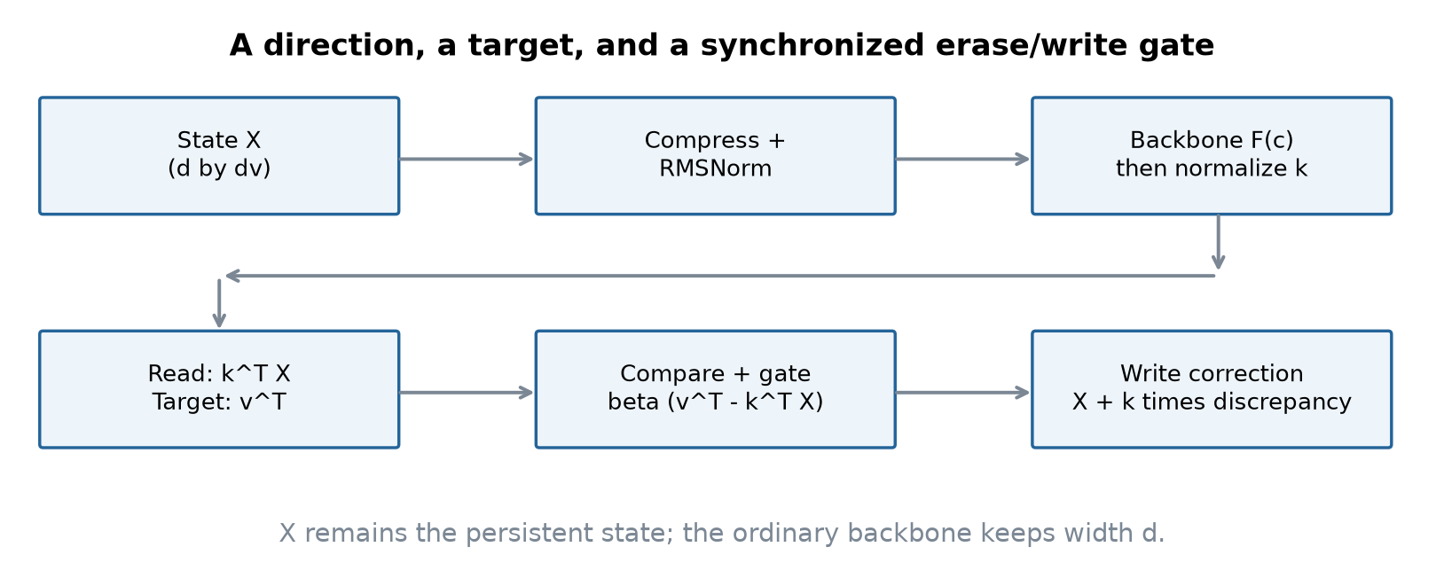
I organize the review around three distinctions. First, an exact identity about a conditioned local update is different from a theorem about the full nonlinear network. Second, improvements from expanded-state models do not isolate the contribution of the erase term. Third, equal training tokens do not mean equal training cost. Keeping these distinctions visible makes the method more interesting, because it turns a compact equation into a set of concrete research questions.

All model results below are reported by the paper. Algebraic examples and resource calculations are explanatory calculations in this review. Proposed experiments are suggestions, not new measurements or reproduced model-training results. The official project link is a resource entry; the analysis here is grounded in the paper and its appendices.

2. Prerequisites: residuals, projections, and the axis of recurrence

2.1 A residual stream is a state passed through depth

For a single token, a conventional residual state is a vector $x_l\in\mathbb{R}^d$. A pre-normalized sublayer computes a transformation from a normalized view of that state and adds its output back:

$$c_l=\operatorname{RMSNorm}(x_l),\qquad x_{l+1}=x_l+F_l(c_l).$$

Attention can mix information across tokens; an MLP transforms features at the current token. Both use the residual interface to communicate with later sublayers. Here $l$ indexes a residual update, so an attention update and an MLP update are separate operations within a Transformer block.

An additive interface does not require monotonically accumulating positive information. The branch can output negative components and cancel existing values. The practical issue is where the architecture places responsibility for learning that cancellation. DDL exposes a readout and a target instead of leaving the entire correction inside an unconstrained vector.

2.2 A unit direction defines a coordinate without changing the basis explicitly

Let $k\in\mathbb{R}^d$ satisfy $k^\top k=1$. The scalar $k^\top x$ is the coordinate of $x$ along $k$. Its vector contribution is $k(k^\top x)$, and the remaining component is

$$x_\perp=x-k(k^\top x),\qquad k^\top x_\perp=0.$$

The matrix $P=kk^\top$ is an orthogonal rank-one projector: $P^2=P$ and $P^\top=P$. This fact is the main linear-algebra ingredient in DDL. It means that an update proportional to $k$ can change the selected coordinate while leaving the orthogonal component unchanged, provided we condition on that direction for the particular update.

For an expanded state $X\in\mathbb{R}^{d\times d_v}$, the same projection acts on every value column. The readout $k^\top X$ is now a row vector with $d_v$ entries. One direction in feature space therefore selects several values at once; it does not select $d_v$ unrelated feature directions.

2.3 Depth recurrence is different from sequence recurrence

Delta-rule sequence models update a memory as tokens arrive. DDL applies analogous algebra as layers update a token representation. The notation is similar, but the recurrent axis changes. DDL still uses standard attention in its reported Transformer backbone; it is not, by itself, a replacement for attention with constant-size recurrent sequence memory.

This distinction matters for systems reasoning. Expanding a residual state says nothing immediate about shrinking the attention KV cache. A token-history compressor can even introduce another small history buffer. The relevant question is which tensors persist across depth, which persist across decoding steps, and which are saved for backpropagation.

3. Deriving the read-compare-write update

Suppress the token and layer indices temporarily. DDL generates a direction $k$, a target $v\in\mathbb{R}^{d_v}$, and a scalar gate $\beta$. With a unit direction, its update is

$$X^+=X+\beta k\left(v^\top-k^\top X\right). \tag{1}$$

Every multiplication has a concrete role. The read $r=k^\top X$ has shape $1\times d_v$. The discrepancy $v^\top-r$ has the same shape. Multiplying it on the left by $k$ produces a $d\times d_v$ correction of rank at most one. The scalar gate scales the entire correction, synchronizing removal of the old readout and insertion of the requested value.

Expanding the parentheses gives the form used for the shortcut analysis:

$$X^+=\underbrace{(I-\beta kk^\top)}_{A}X+\beta kv^\top. \tag{2}$$

The two terms are not independent mechanisms with arbitrary strengths. The same $\beta$ appears in both. To see why this matters, multiply Equation (1) by $k^\top$:

$$\begin{aligned} k^\top X^+ &=k^\top X+\beta(k^\top k)(v^\top-k^\top X)\\ &=(1-\beta)k^\top X+\beta v^\top. \end{aligned} \tag{3}$$

Subtract the target from both sides and define $e=k^\top X-v^\top$. Then

$$e^+=(1-\beta)e. \tag{4}$$

This is the exact local error-correction statement. At $\beta=0$ the whole update is the identity. At $\beta=1$ the selected readout equals the target after the update. When $1<\beta<2$, the readout crosses the target but ends closer to it in magnitude. For $0<\beta<2$, its error norm is multiplied by $|1-\beta|<1$.

If erase and write used separate gates, say $a$ and $b$, the selected readout would instead be $(1-a)r+bv^\top$. At $a=1$, this equals the requested target only when $b=1$, apart from special values of $v$. DDL’s shared gate therefore encodes a useful invariant rather than merely reducing parameter count.

There is also a local optimization interpretation. Freeze $k$ and $v$, and consider the auxiliary objective

$$E(X)=\frac12\|k^\top X-v^\top\|_2^2.$$

Its gradient with respect to $X$ is $\nabla_X E=k(k^\top X-v^\top)$. Equation (1) is one gradient step on this quadratic with step size $\beta$. Because the nonzero eigenvalue of $kk^\top$ is one, the interval $(0,2)$ gives contraction of this selected-coordinate error. This derivation is explanatory: training optimizes the language-model objective, and the generated target itself changes with the input. DDL is not separately minimizing a fixed reconstruction loss at every layer during training.

4. Geometry: preserve, replace, or over-relax

For frozen $k$ and $\beta$, the direct shortcut is $A=I-\beta kk^\top$. If $u$ is orthogonal to $k$, then $Au=u$. Along the selected direction,

$$Ak=k-\beta k(k^\top k)=(1-\beta)k.$$

The eigenvalues are therefore $1$ on the $d-1$ dimensional orthogonal subspace and $1-\beta$ along $k$. At $\beta=0$, all eigenvalues are one and there is no distinguished eigenspace associated with a different eigenvalue. For expanded states, vectorization repeats this operator across value columns; it does not introduce a different shortcut spectrum for each channel.

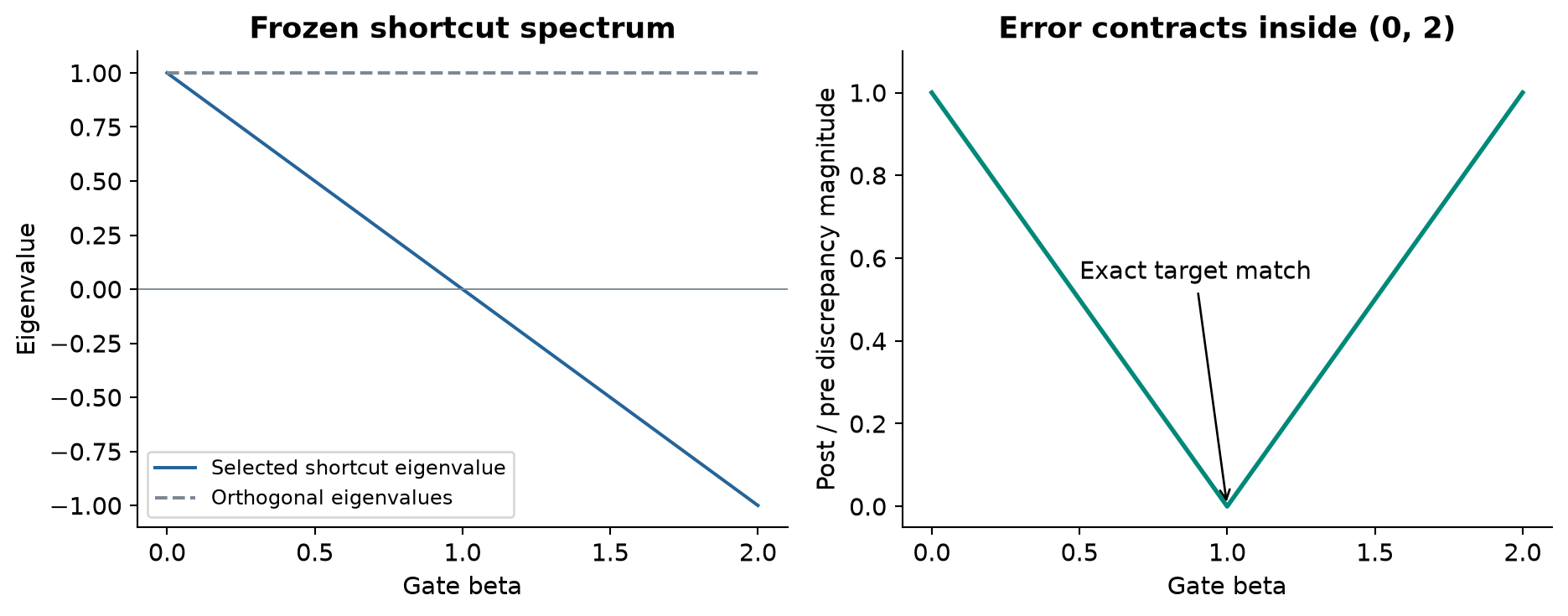
At $\beta=1$, $A=I-kk^\top$ projects away the old selected component. The separate target write restores a new component there. Calling the whole block an orthogonal projection would omit that write and the state dependence of the generators.

At $\beta=2$, the shortcut is a Householder reflector. The full conditioned update is

$$X^+=X-2k(k^\top X-v^\top).$$

For fixed $k$ and $v$, this can be understood column by column as an affine reflection about the target hyperplane, not necessarily a reflection through the origin. For example, if the selected coordinate starts at 4 and the target is 1, the reflected coordinate is $2\cdot1-4=-2$. The magnitude of the residual vector need not be preserved relative to the origin when the target is nonzero.

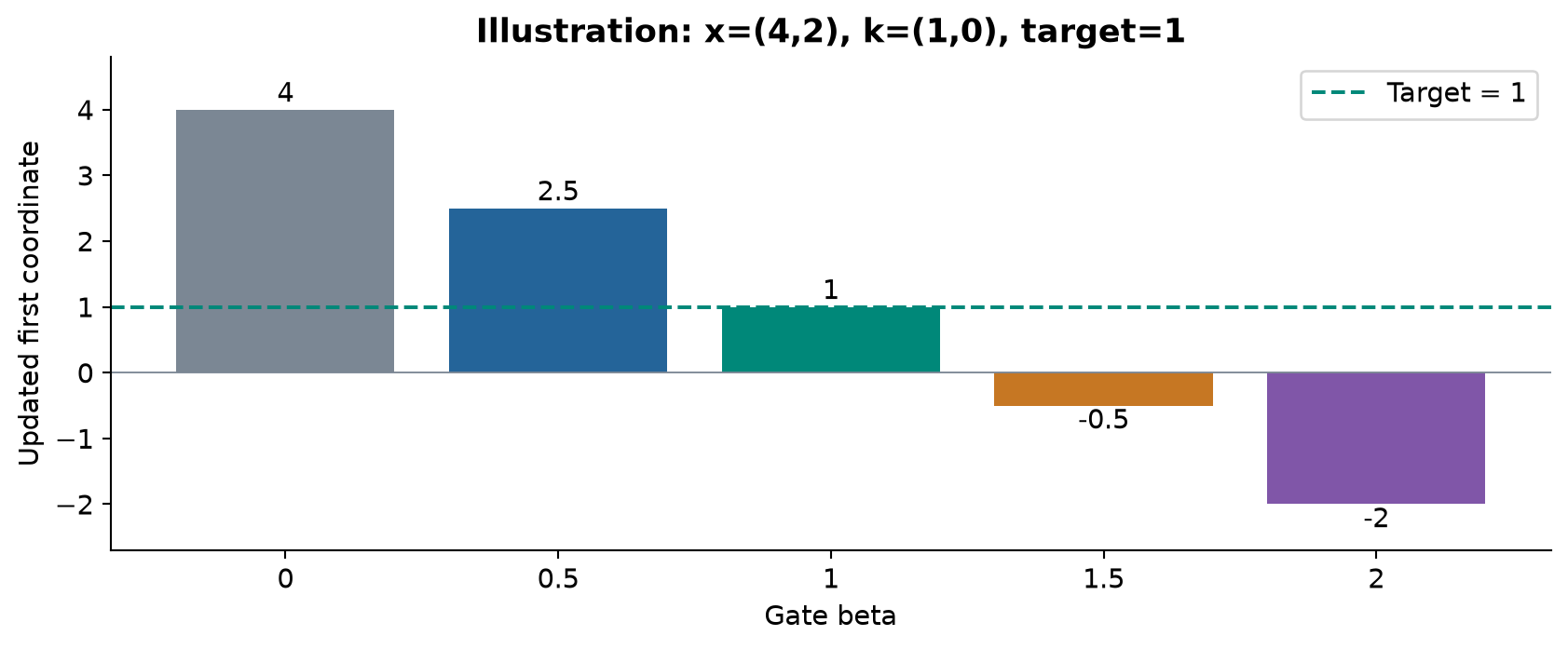
In the paper, $\beta=2\sigma(g(c))$. Finite logits place it inside $(0,2)$; exact zero and two are limiting cases. A small gate favors the identity path but also makes the sigmoid derivative small. A gate near one allows exact matching in the ideal unit-direction algebra and has the largest logit sensitivity. These are local parameterization properties, not evidence that a trained model actually organizes its layers into human-readable skip, overwrite, and reflection roles.

An immediate failure case is a direction unrelated to useful information. DDL can precisely overwrite the wrong readout. Another is an inaccurate target: making the local discrepancy zero is no guarantee that the language-model prediction improves. The architectural invariant makes the operation interpretable as an operation; it does not certify the semantic value of the edit.

5. What the local spectrum does and does not say

5.1 Nonexpansive is not globally contractive

For $d>1$ and $0\leq\beta\leq2$, the spectral norm of the frozen shortcut is

$$\|A\|_2=\max\{1,|1-\beta|\}=1.$$

The selected-coordinate error contracts for interior gates, but the orthogonal coordinates are preserved. Thus even this simplified linear map is not a strict contraction of every perturbation. A product of fixed shortcuts is nonexpansive under these assumptions, although which components shrink depends on the sequence of directions. This is a useful statement about one direct path through the network, not a bound on the entire trained network.

The distinction becomes explicit by differentiating the actual update. Let $w=v^\top-k^\top X$ be the write discrepancy. Allow all three generators to depend on the state. The first-order differential is

$$\begin{aligned} dX^+={}&(I-\beta kk^\top)dX\\ &+(d\beta)kw+\beta(dk)w\\ &+\beta k\,dv^\top-\beta k(dk)^\top X. \end{aligned} \tag{5}$$

The first line is the frozen shortcut. The other lines contain sensitivity through the gate, direction, and target. Their sizes are not bounded just by knowing the eigenvalues of $A$. Attention also couples token positions, so a full sequence Jacobian has additional block structure. The paper’s direct-path geometry helps describe a design choice; it does not establish absence of exploding gradients or a global Lipschitz constant of one.

There is an equally useful forward distinction. For a later readout direction $q$, the current edit changes its value by

$$q^\top X^+-q^\top X=\beta(q^\top k)w. \tag{6}$$

Only readouts orthogonal to the current $k$ are preserved. If a later layer chooses a correlated direction, it sees a changed value. Local orthogonality therefore does not imply stable, independent semantic slots throughout depth. Direction interference is an interesting measurement to make, not something the rank-one formula removes automatically.

5.2 Numerical normalization slightly changes the ideal identity

Appendix A describes a guarded normalization equivalent to

$$k=\frac{h}{\sqrt{\|h\|_2^2+\epsilon_k^2}}.$$

Define $\rho=\|k\|_2^2$. For a nonzero guard, $\rho<1$, approaching one when $\|h\|$ is large relative to $\epsilon_k$. Repeating the projection calculation without substituting unit norm gives

$$\begin{aligned} r^+&=r+\beta\rho(v^\top-r),\\ r^+-v^\top&=(1-\beta\rho)(r-v^\top). \end{aligned} \tag{7}$$

Consequently, exact overwrite at $\beta=1$ is an idealized unit-direction statement. The guarded operation approximates it in the normal regime. When $h=0$, the direction is zero and the rewrite vanishes. This is preferable to division by zero, but it means that “the gate equals one” alone does not certify exact readout replacement.

The normalization has its own sensitivity. With $s=\sqrt{\|h\|^2+\epsilon_k^2}$,

$$D_hk=\frac{I}{s}-\frac{hh^\top}{s^3},\qquad \|D_hk\|_2\leq\frac1s\leq\frac1{\epsilon_k}.$$

The guard limits a singularity; it does not make the bound small. A small backbone output can make direction changes sensitive even while the direct shortcut remains controlled. This provides a concrete reason to distinguish numerical safeguards from a theorem about optimization stability.

6. From the equation to a complete residual interface

6.1 Direction, target, and gate come from different paths

DDL first compresses the state to the usual model width and applies RMS normalization:

$$x_{\mathrm{in}}=C(X),\quad c=\operatorname{RMSNorm}(x_{\mathrm{in}}),\quad h=F(c),\quad v=W_vc.$$

Here $F$ is the existing attention or MLP branch. Its output supplies the unnormalized direction $h$; DDL does not require a second independent direction network. The target projection produces $d_v$ values from the normalized context. A gate network produces a scalar, transformed as $\beta=2\sigma(g_\beta(c))$. The paper allows a linear gate or a small two-layer gate with a tanh hidden activation.

These paths impose an interesting division of labor. A high-dimensional sublayer chooses where to edit, while a compact target branch specifies the values written along that direction. Normalizing $h$ removes its overall magnitude from the direction. Update magnitude then depends on the discrepancy and gate. This differs from an ordinary residual branch, where the norm of $F(c)$ directly scales the addition. It is one reason a successful comparison cannot attribute every difference to the explicit erase term alone.

The appendix describes initializing the gate bias through $\operatorname{logit}(\beta_0/2)$, with clamping for numerical safety, and using float32 gate logits. This review does not assign an undocumented default value to $\beta_0$. Initializing near zero makes the block close to identity but can reduce gate sensitivity; initializing closer to one emphasizes correction. Those tradeoffs should be measured under a common initialization protocol.

6.2 Algorithm 1: one forward residual update

Inputs: expanded state $X\in\mathbb{R}^{d\times d_v}$, compressor $C$, backbone sublayer $F$, target projection $W_v$, gate network $g_\beta$, and positive normalization guard $\epsilon_k$.

1. Compress: calculate $x_{\mathrm{in}}\leftarrow C(X)$, using only available tokens if $C$ uses temporal context.
2. Normalize context: calculate $c\leftarrow\operatorname{RMSNorm}(x_{\mathrm{in}})$.
3. Process: calculate $h\leftarrow F(c)$; attention may consult the normal causal attention state.
4. Generate direction: set $k\leftarrow h/\sqrt{\|h\|_2^2+\epsilon_k^2}$.
5. Generate target and gate: set $v\leftarrow W_vc$ and $\beta\leftarrow2\sigma(g_\beta(c))$.
6. Read: calculate $r\leftarrow k^\top X$.
7. Compare: calculate $w\leftarrow v^\top-r$.
8. Rewrite: return $X^+\leftarrow X+\beta kw$.

The sequence is conceptual pseudocode, not a claim about a particular kernel schedule. Reads, discrepancy calculation, and writes can be fused to reduce intermediate traffic. The expanded state is not compressed permanently: the compressor generates a view for the sublayer, and the rewrite acts on the full state. Compressing and then replacing the state with only $x_{\mathrm{in}}$ would describe a different architecture.

6.3 Channel and token compression make different promises

The experiments use $d_v=4$ for expanded DDL. The channel compressor, CC, mixes value channels separately for each feature at the current token:

$$(x_{\mathrm{in},t})_i=\sum_{j=1}^{d_v}a_{i,j}X_{t,i,j}. \tag{8}$$

This is a learned linear reduction of the value dimension. It leaves the width supplied to attention and the MLP equal to $d$. It adds no per-layer history across tokens for this compression operation.

The token compressor, TC, first applies a causal short convolution independently to expanded features, then projects value channels:

$$\begin{aligned} \widetilde X_{t,i,j}&=\sum_{s=0}^{K-1}a_{i,j,s}X_{t-s,i,j},\\ (x_{\mathrm{in},t})_i&=\sum_j p_j\widetilde X_{t,i,j}. \end{aligned} \tag{9}$$

The stated default channel projection starts at uniform weights $1/d_v$. Causal padding handles the start of the sequence. TC exposes local temporal information before the expensive backbone and requires history during autoregressive decoding. This extra communication may affect accuracy as well as cost; it is not merely an alternative implementation of the same mathematical view.

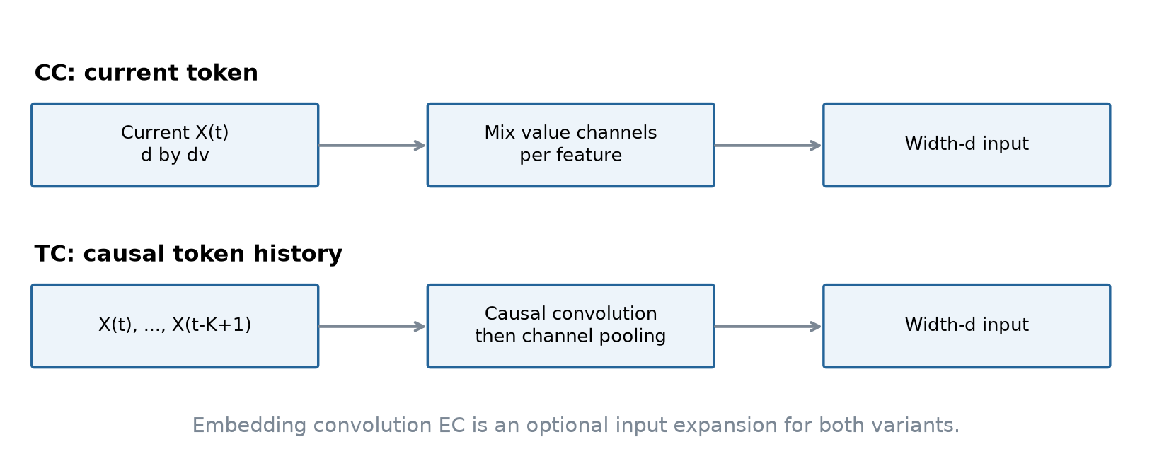
The embedding expansion convolution, EC, is a separate component. It transforms the embedding stream of width $d$ into $d\,d_v$ channels with a depthwise causal short convolution, then reshapes it into the expanded state. The paper describes identity initialization that initially behaves like repetition. Without EC, the initial embedding is repeated across value channels. Removing EC does not remove the expansion itself, and retaining EC with CC can still require a small embedding-stage history buffer. “CC has no TC history” is more precise than “CC needs no history anywhere.”

These distinctions help read the ablations correctly. A no-EC row tests the input expansion mechanism. A TC-versus-CC row changes the per-sublayer compressor. A scalar-DDL row removes value expansion. None of these, on its own, is a matched removal of the erase term with every other component held fixed.

7. Storage and arithmetic: where the extra capacity lives

7.1 An expanded residual state is not an expanded backbone

A live residual tensor stores $BTdd_v$ elements for batch size $B$ and sequence length $T$. At $s$ bytes per element, its raw size is

$$M_{\mathrm{state}}=BTdd_vs. \tag{10}$$

For an illustrative single sequence with $T=1024$, $d=1024$, $d_v=4$, and two-byte elements, this is 8 MiB, compared with 2 MiB for a scalar state. This calculation covers one live state only. It is not the paper’s measured peak training memory: that also depends on saved activations, attention, parameters, gradients, optimizer state, and execution policy.

Attention and MLP inputs remain width $d$, so their large weight matrices do not all grow by a factor of four. The read and rank-one write cost order $dd_v$ operations per token. CC is also order $dd_v$, and a straightforward TC costs order $Kdd_v$. Compared with dense width transformations, these can be small in arithmetic count while remaining significant in memory traffic, reductions, and kernel-launch overhead.

Materializing a projector $kk^\top$ would create a $d\times d$ tensor and defeat the rank-one formulation. Algorithm 1 instead computes a length-$d_v$ readout and an outer-product update. The paper describes optimized kernels for its reported system, including CC and EC. Their reported performance is evidence about those measured configurations; the algebra alone does not imply the same speed on every GPU or framework.

7.2 Decoding requires a separate accounting

For a temporal kernel of length $K$, TC must retain up to $K-1$ expanded token states per update. Its raw history size is order

$$M_{\mathrm{TC\ history}}=B(K-1)dd_vs.$$

As an illustrative calculation, $B=1$, $K=3$, $d=1024$, $d_v=4$, and two-byte storage imply 16 KiB for one such update’s history. The example is not a claim about the paper’s chosen kernel length. To estimate an actual model, multiply by the relevant updates and include buffering conventions, batch size, KV caches, and the separate EC history if present.

The expanded state is a representation within depth; the attention KV cache stores information needed across decoding steps. One does not replace the other. A deployment that is already constrained by KV-cache capacity may gain little from an architectural change that improves residual expressivity while retaining ordinary multi-head attention.

Finally, throughput depends on which bottleneck dominates. A memory-intensive compressor may be tolerable when large backbone matrix multiplications dominate training, yet relatively expensive in a small-batch decoding loop. That is why training throughput, inference throughput, and memory must remain separate measurements. A single parameter-count comparison cannot summarize the systems tradeoff.

8. Experimental design and the validation-loss evidence

8.1 What is held constant

The paper trains Llama-style models on FineWeb-Edu at approximately 124M and 353M parameters. The small configuration uses 12 layers, width 768, and six attention heads; the medium configuration uses 24 layers, width 1024, and eight heads. Both have head dimension 128. The backbone uses RoPE, SwiGLU, and query/key normalization. The small cost table rounds the parameter count to 123M; this is the same small-model comparison, not an additional scale.

Each configuration gets 100,000 optimizer steps, a global batch of 480 sequences, and sequence length 1024. Multiplying these quantities gives

$$N_{\mathrm{tokens}}=100000\times480\times1024=49.152\times10^9.$$

Each run uses four NVIDIA H200 GPUs. The shared recipe uses a $10^{-3}$ learning rate, cosine decay, 2,000 warmup steps, and AdamW with weight decay 0.1 and moment coefficients $(0.9,0.95)$. Gradient clipping is 1.0, dropout is zero, and ordinary backbone biases are disabled while the DDL gate retains its initialized bias. The methods share a $\mu$P-style parameterization. These choices make the recipe comparable but do not mean each architecture receives exhaustive hyperparameter tuning.

The central experimental limitation is simple: one training run is reported for each configuration. There are no seed-level standard errors for the loss differences. Consequently, the tables can rank the observed runs but cannot tell us how often that ranking would repeat.

8.2 Expansion gives the larger point improvements

The following loss values reproduce Table 3. A lower value is better; no confidence intervals are implied.

Variant	Small loss	Medium loss
Baseline	2.8543	2.6053
Scalar DDL	2.8482	2.6039
DDL-TC without EC	2.8355	2.5927
DDL-CC without EC	2.8321	2.5790
DDL-TC	2.8299	2.5905
DDL-CC	2.8329	2.5758

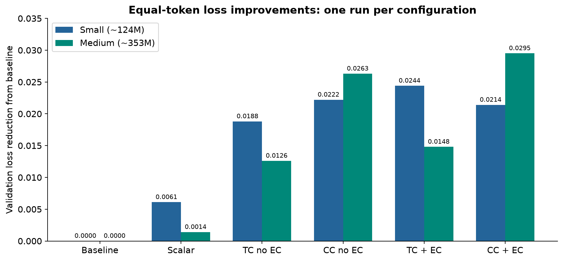
Scalar DDL reduces loss by 0.0061 at the small scale and 0.0014 at the medium scale. The consistent sign is encouraging, but the medium difference is especially small. Without variation across seeds, a claim that scalar rewriting reliably improves pretraining would exceed the evidence.

Expanded models show larger differences. Small DDL-TC improves by 0.0244; medium DDL-CC improves by 0.0295. The corresponding reported perplexities are 16.9438 versus 17.3616 at the small scale and 13.1420 versus 13.5356 at the medium scale. Perplexity is an exponential transformation of mean negative log likelihood, so it should not be treated as an independent second experiment confirming the loss result.

For example, a loss decrease of $\Delta L=0.0295$ implies a perplexity ratio close to $\exp(-0.0295)\approx0.971$. This is about a 2.9% relative reduction in perplexity. It does not mean 2.9% more downstream questions are answered correctly, because the metrics measure different properties.

The EC ablation is also nuanced. Small CC without EC has loss 2.8321, slightly lower than CC with EC at 2.8329. Medium CC benefits from EC in the reported run, improving from 2.5790 to 2.5758. TC improves with EC at both scales. The evidence does not support a universal rule that adding EC always improves every variant; it supports examining the combined architecture and its cost.

9. Downstream evaluation: a better average can hide reversals

The paper uses lm-evaluation-harness with eight reported columns: ARC-C, ARC-E, HellaSwag, OpenBookQA, PIQA, SciQ, Social IQA, and WinoGrande. Tables 1 and 2 give one-shot results; Appendix D gives zero-shot results. The two settings should be examined separately rather than merged into one headline.

Variant	Small 1-shot	Small 0-shot	Medium 1-shot	Medium 0-shot
Baseline	48.56	47.30	53.96	51.92
Scalar DDL	48.73	47.32	54.69	51.94
TC without EC	48.91	47.54	54.83	52.22
CC without EC	49.13	47.07	54.92	52.88
TC	49.47	47.83	54.86	52.87
CC	49.29	47.18	55.14	52.85

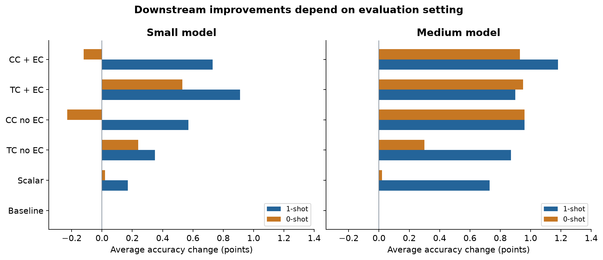
Small CC improves the one-shot average by 0.73 percentage points yet reduces the zero-shot average by 0.12 points. Small TC has the best one-shot average, 49.47, and improves zero-shot by 0.53 points. At the medium scale, CC has the best one-shot average, 55.14, while CC without EC has the highest zero-shot average by a very small margin. Different objectives choose different rows.

Even medium CC’s favorable one-shot average is not uniform task dominance. Compared with the baseline, its ARC-E score falls from 67.05 to 65.57 and PIQA falls from 70.24 to 69.48. OpenBookQA rises from 33.20 to 36.00, SciQ from 87.30 to 90.50, and WinoGrande from 52.57 to 55.72. These numbers explain how a positive macro average can coexist with meaningful task-level regressions.

A macro average weights each benchmark column equally, including the two ARC subsets. That is a reporting convention, not a deployment utility function. An application whose failures resemble ARC-E or PIQA may care about the regressions more than the aggregate gain. Conversely, an application closer to the improved tasks might find the tradeoff attractive. The paper establishes neither conclusion for a particular application.

No repeated-seed distribution is available for these pretrained models. Prompt setting and benchmark sampling can add further variation beyond training randomness. The right use of this table is to identify promising configurations and fragile claims, then test a relevant evaluation set. It is not evidence that DDL generally improves reasoning, all knowledge tasks, or every prompt regime.

10. A systems reading of the cost tables

10.1 Throughput is a measured cost, not a footnote

Tables 4 and 5 report training and inference throughput on the same hardware and software stack, with optimized Triton kernels for CC and EC-enabled implementations. The numbers are hardware-specific point measurements. The paper does not report end-to-end pretraining GPU-hours or total forward/backward FLOPs, and the table headings do not by themselves specify a production serving latency target or traffic distribution.

The default CC variant gives the following comparison. Throughput is in thousands of tokens per second, as labeled in the source tables.

Scale and variant	Train Ktok/s	Inference Ktok/s	Peak memory
Small baseline	1509.6	1826.1	2.94 GB
Small CC	1158.0	1220.7	3.08 GB
Medium baseline	537.1	531.5	7.06 GB
Medium CC	422.3	400.5	7.20 GB

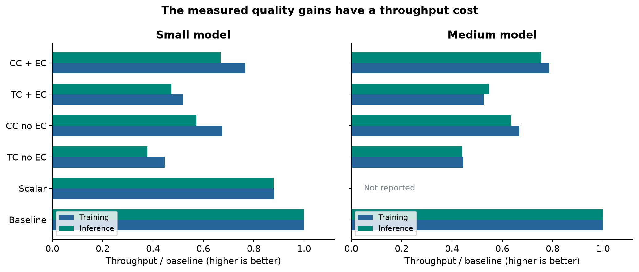
Small CC retains about 76.7% of baseline training throughput and 66.8% of inference throughput. Medium CC retains about 78.6% and 75.4%, respectively. Calling the train-throughput reduction “23.3% slower training” is ambiguous: for a fixed token count, time is the reciprocal of throughput. The corresponding idealized time multipliers are about 1.304 and 1.272, before accounting for any unmeasured end-to-end overhead.

Small scalar DDL already reduces train throughput from 1509.6 to 1330.8 Ktok/s, despite unchanged rounded peak memory and parameter count. This is a concrete reminder that additional reductions and elementwise operations can cost time without making a model look much larger in a parameter table. The medium cost table has no scalar-DDL row; filling it by scaling the small result would invent a measurement.

TC is more expensive in the measured configurations. With EC, small TC reaches 783.5 Ktok/s for training and medium TC 282.9 Ktok/s, approximately 51.9% and 52.7% of their baselines. The small loss minimum therefore comes with a substantial cost. Selecting CC as the paper’s default is a quality-efficiency judgment across metrics, not a statement that CC wins every quality column.

10.2 Memory needs a denominator and a workload

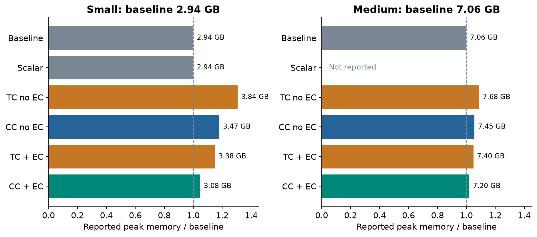
The small CC peak increases from 2.94 to 3.08 GB, about 4.8%; medium CC increases from 7.06 to 7.20 GB, about 2.0%. This does not contradict a fourfold increase in the raw residual state: the state is only one part of total peak memory, and the execution schedule affects overlapping intermediates.

The no-EC rows also caution against treating a component name as a monotonic resource prediction. Small CC without EC reports 3.47 GB and 1019.8 Ktok/s training, compared with 3.08 GB and 1158.0 for CC with EC. The source explicitly distinguishes optimized paths. These measurements describe whole execution configurations; they do not prove that adding a convolution intrinsically reduces arithmetic or memory. A fair kernel-level explanation would require a different experimental decomposition, which is outside the evidence presented here.

10.3 What would equal time mean?

Let $q=T_{\mathrm{DDL}}/T_{\mathrm{base}}$ denote a ratio of token throughputs, with $T$ here meaning throughput rather than sequence length. If the reported rates held throughout training and all other overheads matched, DDL would process $qN$ tokens while the baseline processes $N$ tokens. For CC and $N=49.152$ billion, this gives approximately 37.70 billion small-model tokens or 38.65 billion medium-model tokens.

This arithmetic is a budget illustration, not a result from additional training runs. It cannot tell us the final loss at those token counts under a properly adjusted schedule. In particular, keeping a 100,000-step cosine schedule but stopping it early differs from training a shorter schedule to completion. Nor does multiplying loss reduction by a throughput ratio produce a meaningful “efficiency score.”

A convincing equal-time comparison would log actual elapsed training time, include relevant communication and checkpoint overheads, and compare complete schedules. An equal-FLOPs comparison would separately measure or estimate forward/backward arithmetic under stated conventions. A serving comparison would need batch size, context length, generation length, and latency constraints. The paper’s tables are useful starting points for all three, but are not substitutes for them.

11. Limitations and failure boundaries

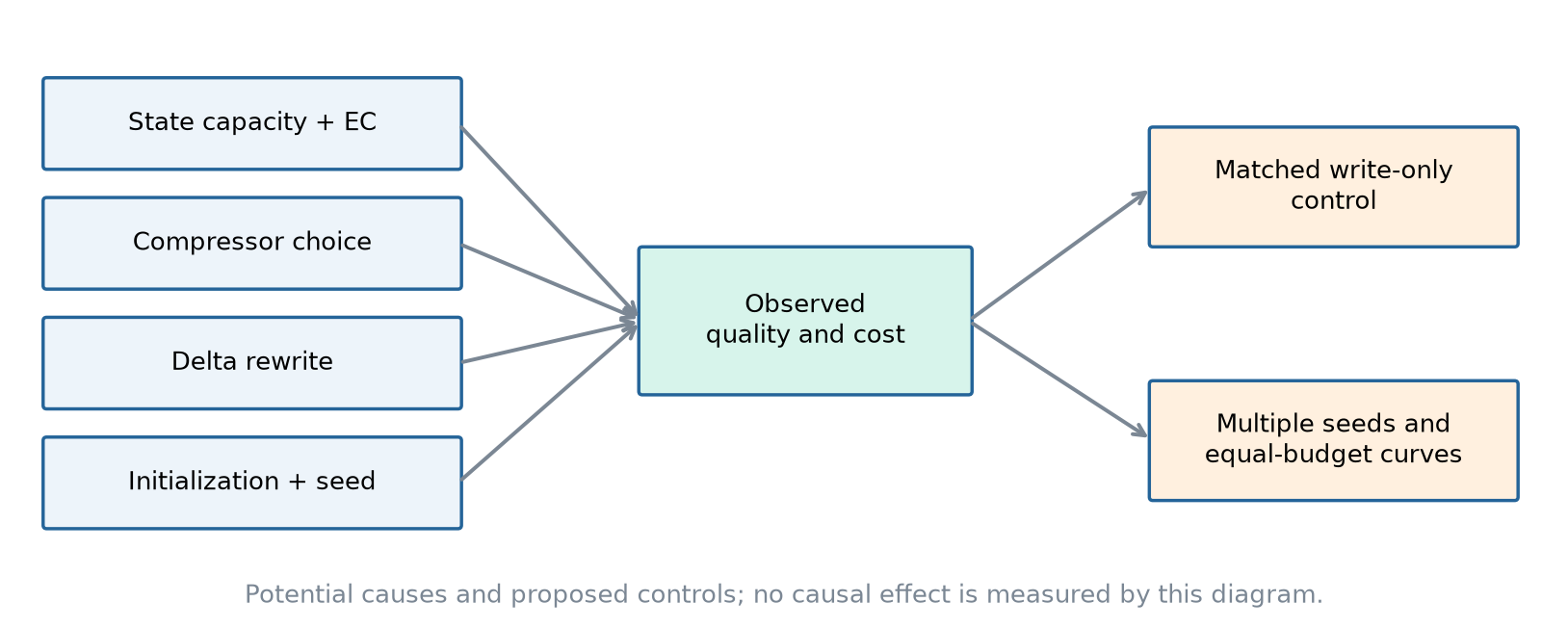
The v4 manuscript explicitly acknowledges its most important empirical boundaries. It reports one seed per configuration, does not isolate delta rewriting within the expanded state, lacks equal-FLOPs and equal-time comparisons, and limits interpretability to the conditioned operator. These are not omissions discovered by this review; they are constraints the authors already place on their conclusions.

First, the smaller scalar-DDL loss differences may lie within training variation. The observed sign is not enough to establish a reliable benefit. Multiple paired runs would be particularly valuable here, because the scalar setting comes closest to testing the residual rule without expanded storage.

Second, the strongest expanded-state results combine several changes: four value channels, a compressor, the direction/target/gate interface, and usually EC. The no-EC ablation removes one factor but leaves the others. It supports saying that EC is not necessary for a positive loss point difference; it cannot identify how much improvement comes from subtracting the old readout.

Third, the experiments cover relatively small models and a 1024-token pretraining sequence length. They do not establish scaling behavior at multi-billion-parameter scale, long-context stability, performance after instruction tuning, or latency in a production decoder. The idea could transfer, but the current paper does not measure those claims.

Fourth, a normalized direction can be unhelpful, a target can be wrong, and a learned gate can saturate. Exact local editing remains exact editing of whatever values the model generates. The equation alone does not ensure useful semantic selection. The guarded normalization also introduces a regime where the ideal unit-norm identity becomes approximate.

Fifth, changes in software paths and hardware bottlenecks can alter the measured quality-cost compromise. The table reports real overhead, but does not provide enough end-to-end information to select a deployment configuration for a new workload. The missing medium scalar cost measurement further limits comparison of the simpler alternative.

Finally, the reported gains should not be broadened into a claim that the delta rule itself is new. The contribution is its use as a depth-wise residual interface and the expanded-state architecture around it. Similarly, channel mixing is a component choice, not an independent novelty claim. These distinctions keep the paper’s contribution aligned with what it actually develops and measures.

12. Independent critical analysis

12.1 The next decisive comparison is a matched write-only model

The authors themselves propose a write-only control. I agree with that priority because it directly addresses the central causal ambiguity. Preserve $d_v$, EC, the compressor, the branches generating $k,v,\beta$, initialization, optimizer, and data order, then remove only the state-dependent read-and-erase term:

$$X^+_{\mathrm{write}}=X+\beta kv^\top.$$

Algorithm 2: a proposed paired attribution experiment.

1. Select a fixed expanded configuration, such as CC with $d_v=4$, and define its complete training budget.
2. Initialize paired DDL and write-only models from matched parameter draws and gate settings wherever their structures coincide.
3. Feed identical ordered training data under the same optimizer schedule; repeat this pairing over multiple seeds.
4. Use Algorithm 1 for the DDL arm. In the control arm, omit the read in step 6 and replace the final correction with $\beta kv^\top$.
5. Record validation loss, benchmark scores, elapsed time, memory, and cumulative compute at common checkpoints.
6. Report distributions of paired differences and separately compare equal-token and equal-resource checkpoints.

This is a proposed experiment, not a result in the current paper or a run performed for this review. Its value is that both arms retain the normalized backbone direction and compact target generation. Comparing DDL only with a conventional additive block simultaneously changes these branch roles, so it cannot isolate the erase operation cleanly.

Even this control needs care. Removing the read changes initial update statistics and possibly the amount of useful computation per step. Reporting those differences is preferable to silently adjusting one arm until it wins. A second set of fairly tuned runs could test each architecture’s best performance, but that answers a different question from a strict component attribution study.

12.2 A tautological diagnostic is not a semantic explanation

Plotting $\|k^\top X^+-v^\top\|$ before and after the update may verify the algebraic operating regime, including normalization effects. But with a unit direction its ratio is already determined by $|1-\beta|$. Observing the expected reduction would not independently demonstrate that the model learned a useful concept or erased harmful information.

A stronger diagnostic would relate gate behavior and direction interventions to held-out task loss. For example, hold a layer’s generated target fixed while changing the selected direction, or restrict a subset of updates and measure prediction degradation under carefully specified interventions. Such experiments must account for distribution shift: arbitrarily perturbing a representation can damage any model. The question is whether the proposed interpretation predicts effects better than simple norm or layer-depth explanations.

Equation (6) suggests another measurement: how strongly one edit alters later readouts through direction correlations. A system could make individually simple corrections that interfere substantially across layers. Conversely, it might organize near-orthogonal edits. The present results do not distinguish these possibilities. That is a more informative open question than assuming geometric transparency equals semantic disentanglement.

12.3 Capacity must be used, not just allocated

Expanded states start with repeated or identity-expanded embeddings. Allocating four value channels does not ensure four independent information channels. The target projection and subsequent updates can create diversity, but whether they do so effectively is empirical.

One useful analysis would measure the spectrum of centered channel covariances across tokens and layers, alongside compressor outputs and task quality. If most channel variation remains nearly redundant, the storage expansion may act mainly through altered optimization or local transformations. If meaningful diversity develops and predicts quality, that would strengthen the capacity interpretation. A covariance spectrum alone would still not prove causal usefulness; a controlled reduction of channel capacity would be needed to connect the two.

This matters for choosing alternatives. A slightly wider additive model, a different residual mixing design, or a smaller number of expanded channels might offer a better resource frontier. The fairest comparator for an engineering decision is a model at the same practical budget, not necessarily one with the same rounded parameter count. The paper’s close parameter counts are informative about where capacity is stored, but are not a complete fairness criterion.

12.4 The useful outcome is a quality-cost frontier

There is no single winning row across loss, one-shot accuracy, zero-shot accuracy, training speed, and inference speed. Small TC has the best loss and one-shot average but much lower throughput. Medium CC looks attractive on loss and one-shot average, yet still incurs measured overhead. Small CC’s zero-shot average is below the baseline.

My preferred follow-up would plot validation loss against actual training time, then separately plot task quality against inference cost for relevant workloads. This would make an architectural decision concrete: how much resource buys how much improvement, and which tasks regress? Add repeated seeds and the matched write-only control, and the paper’s most interesting hypothesis becomes testable without relying on a broad “better residual connection” headline.

13. Conclusion

Deep Delta Learning offers a compact residual interface with a clear local meaning: read a coordinate, compare it with a generated target, and apply a gated rank-one correction. The ideal unit-direction formulation gives exact statements about selected-coordinate replacement and the frozen shortcut spectrum. Expanded residual storage then separates representational width from the width used by expensive backbone operations.

The reported experiments support a narrower but useful empirical conclusion. Expanded DDL configurations improve validation loss in the measured equal-token runs and often improve one-shot averages, while costing throughput and sometimes increasing peak memory. The scalar improvements are small, zero-shot results are mixed, and the expanded-state results do not yet isolate the erase term or establish an equal-compute advantage.

The paper is worth reading for the interface and for the research questions that interface makes precise. The next evidence needed is equally concrete: matched write-only controls, repeated training seeds, actual equal-resource curves, and measurements connecting learned edits to useful predictions. Until then, DDL is a promising quality-cost tradeoff to investigate, rather than a demonstrated shortcut to cheaper pretraining.

References and figure provenance

1. Yifan Zhang, Yifeng Liu, Mengdi Wang, and Quanquan Gu. Deep Delta Learning. arXiv:2601.00417v4, July 27, 2026. Abstract and version history; complete paper. All architecture descriptions and model measurements in this review refer to this version, including Appendices A-D.
2. Official Deep Delta Learning project. Resource link supplied with the paper.

Figures 1, 4, and 9 are original explanatory diagrams based on the reviewed method and the analysis above. Figures 2 and 3 plot analytic examples, not trained-model observations. Figures 5-8 redraw values from Tables 1-5 and Appendix D; no missing measurements are interpolated. Storage and equal-time examples are labeled calculations in this review. No new training, reproduction result, or confidence interval is claimed.