Gated Attention: Controlling What a Softmax Head Writes

Review date: September 23, 2026
Author: Zhongzhu Zhou
Paper: Gated Attention for Large Language Models: Non-linearity, Sparsity, and Attention-Sink-Free
Paper authors: Zihan Qiu, Zekun Wang, Bo Zheng, Zeyu Huang, Kaiyue Wen, Songlin Yang, Rui Men, Le Yu, Fei Huang, Suozhi Huang, Dayiheng Liu, Jingren Zhou, Junyang Lin
Reading version: NeurIPS 2025 proceedings, 27 pages, including supplementary material and checklist. The arXiv record, 2505.06708, was first submitted on May 10, 2025; its 17-page v1 is a different document. Table and figure numbers below refer to the proceedings.
Resources: Proceedings entry · Official code resource

1. The central idea: retrieval and writing need separate controls

A softmax attention head must distribute a total probability mass of one over the available tokens. That is a useful way to select information, but it does not directly express a different decision: how much should this head contribute to the current residual stream? Even when no retrieved content is useful, the weights still sum to one. The model can compensate through its value vectors, output projection, interactions between heads, or learned attention patterns. A gate gives it a more direct control.

The main successful variant in this paper applies a sigmoid gate after the attention-weighted value sum and before the output projection. The gate depends on the current token’s hidden state and can differ across query heads and feature coordinates. The modification is compact, yet the authors evaluate enough alternatives to make placement and granularity meaningful research questions rather than incidental choices.

The strongest reported configuration reduces average perplexity from 6.026 to 5.761 in the 15B MoE experiment trained on 400B tokens. It also improves several downstream scores, supports more aggressive learning rates in selected dense-model settings, and loses substantially less RULER performance after a particular positional extrapolation procedure. These are useful results. Their scope is the tested architectures, data and training recipes; a gate is not a general guarantee of better accuracy or lower inference cost.

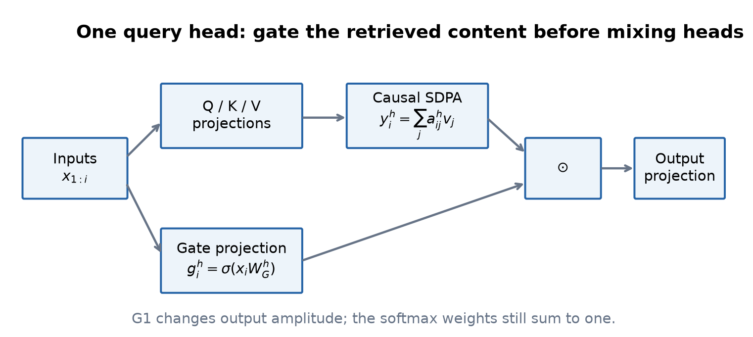
Three distinctions organize this review. First, suppressing an activation is different from skipping the computation that produced it. Second, introducing an input-dependent map is different from increasing the rank of every fixed matrix in that map. Third, an attention sink disappearing in a trained model is different from a gate algebraically removing a sink in the same forward pass. Keeping these distinctions explicit makes the paper more informative for architecture and systems decisions.

The paper’s contribution is best understood as a systematic study of a small architectural degree of freedom. It compares gates on queries, keys, values, attention outputs and dense outputs; it tests different granularities, nonlinearities and shared-head constraints; and it studies associated activation and attention statistics. Earlier work already used gates in several model families. The value here lies in the controlled placement study and the attempt to connect performance with training behavior.

All benchmark values in this review are reported paper values. The diagrams, algebraic examples and arithmetic conversions are original explanations. They are not new training experiments or evidence of reproduced model performance.

2. Prerequisites: the maps inside one attention layer

2.1 Queries choose; values carry; the output projection combines

Use row-vector notation. Let $x_i\in\mathbb R^d$ be the normalized representation at position $i$, and let $h$ index a query head. A grouped-query attention layer can share a key/value head among several query heads. Write $r(h)$ for the key/value group associated with head $h$. The projections are

$$q_i^h=x_iW_Q^h,\qquad k_j^{r(h)}=x_jW_K^{r(h)},\qquad v_j^{r(h)}=x_jW_V^{r(h)}.$$

The paper’s architectures also use query/key normalization and rotary position embeddings. Those operations belong in the query/key path; they are omitted in this first expression to expose the value/output structure. With the appropriate positional transformations included in $q$ and $k$, causal attention gives

$$\begin{aligned} s_{ij}^h&=\frac{q_i^h(k_j^{r(h)})^\top}{\sqrt{d_h}},\qquad j\le i,\\ a_{ij}^h&=\frac{\exp(s_{ij}^h)}{\sum_{t\le i}\exp(s_{it}^h)},\\ y_i^h&=\sum_{j\le i}a_{ij}^h v_j^{r(h)}. \end{aligned}$$

Each $y_i^h$ has head width $d_h$. Concatenate head outputs and multiply by the output projection. Equivalently, partition that projection into row blocks $W_O^h\in\mathbb R^{d_h\times d}$ and sum their contributions:

$$o_i=\operatorname{Concat}_h(y_i^h)W_O =\sum_h y_i^hW_O^h.$$

This equivalence matters. Heads are concatenated before the shared output projection; the resulting projected contributions add in model space. Treating the projected contributions as a second concatenation would give the wrong output dimension and confuse the rank argument later.

2.2 What an attention sink measures

An attention sink is a token or small set of tokens that receives substantial attention mass across many contexts, even when its semantic content is not the relevant retrieval target. The paper mainly diagnoses this through attention allocated to the first token. Its F-Attn statistic averages first-token attention across the measured heads and layers. A value such as 0.467 summarizes a particular evaluation, not a claim that every head always gives exactly 46.7% to the first token.

The normalization constraint helps motivate sinks: if a head would prefer to contribute little, assigning probability to an innocuous token can be a learned workaround. But this is a hypothesis about a trained network. The existence of normalization alone does not prove that sinks must emerge. Values could already be small, or different contributions could cancel. Likewise, a first token can contain legitimately useful context. A lower first-token statistic is a mechanism diagnostic, not a stand-alone quality metric.

2.3 Perplexity, accuracy and efficiency answer different questions

Perplexity is the exponential of average negative log likelihood. If the same evaluation distribution is used, reducing perplexity from $P_0$ to $P_1$ corresponds to the following average log-loss difference:

$$\Delta\mathrm{NLL}=\log P_0-\log P_1=\log\frac{P_0}{P_1}.$$

For 6.026 versus 5.761, this is about 0.04497 nats per token, or a 4.40% relative perplexity decrease. Neither number is a 4.40-point accuracy increase. Benchmark accuracies, training stability and decoding throughput must be considered on their own scales.

Efficiency also has several denominators. A more reliable training recipe might reduce wasted runs without making a forward pass faster. Better quality at fixed token count might improve a quality/compute frontier even if each step becomes slightly more expensive. A smaller average gate does not by itself imply smaller KV storage. These distinctions are particularly important because the paper sits naturally in an Efficient ML reading list while its central intervention adds a computation.

3. The gate and the alternatives it competes with

3.1 G1: query-dependent output modulation

For a head-specific, elementwise gate, define

$$g_i^h=\sigma(x_iW_G^h)\in(0,1)^{d_h},\qquad z_i^h=y_i^h\odot g_i^h.$$

The output becomes

$$o_i^{\mathrm{gate}}=\sum_h z_i^hW_O^h =\sum_h (y_i^h\odot g_i^h)W_O^h.$$

The current position controls the gate. Two queries can retrieve the same historical values but suppress different coordinates of their resulting vectors. This gives the gate a role distinct from the attention distribution: attention chooses a mixture over positions, while the output gate modulates the resulting feature vector.

The sigmoid supplies a bounded, nonnegative multiplier. It can preserve a component approximately, attenuate it, or nearly suppress it. It cannot directly multiply by a negative number or amplify a coordinate above its pre-gate magnitude. The output projection and the rest of the trained network remain free to change scale and sign, so this local bound is not a bound on the full layer’s output norm relative to a separately trained baseline.

3.2 Headwise and head-shared are different restrictions

A headwise gate uses one scalar $\gamma_i^h$ for all coordinates of a head. It still permits different heads to react differently to a query. An elementwise gate allocates a separate scalar to every head coordinate. This is more expressive and substantially more expensive in gate parameters.

Head-shared gating instead forces different query heads to use the same gate values. It reduces independence between heads. In the paper’s reported head-shared construction, scores are obtained by averaging across the query-head dimension of a full projection; its parameter count is therefore not the same as that of a minimal directly projected shared gate. One should not read “shared” in Table 1 as an automatic promise of parameter savings.

These two restrictions ask different questions. Headwise versus elementwise tests whether within-head selectivity matters. Head-specific versus head-shared tests whether distinct retrieval channels need distinct controls. The paper finds that retaining separate controls for different heads is particularly useful, while the much smaller headwise variant remains competitive.

3.3 Why the placement sweep is informative

The authors examine five locations. G1 gates the SDPA output. G2 gates the value projection. G3 and G4 gate the key and query projections. G5 gates after the dense output projection. These changes affect different mathematical objects:

Position	Object changed	Immediate consequence
G1	Current query’s retrieved vector	Query-dependent control before heads mix
G2	Each source token’s value	Source-dependent content changes for future queries
G3	Keys	Changes attention logits and competition among tokens
G4	Queries	Changes attention logits for the current retrieval
G5	Projected model-space output	Controls coordinates after head contributions combine

G2 is not equivalent to G1. Its gate is attached to each historical source token, so it enters inside the weighted sum. In general,

$$\sum_j a_{ij}(v_j\odot g_j) \ne \left(\sum_j a_{ij}v_j\right)\odot g_i.$$

Equality can hold under special conditions, such as all contributing source gates equaling the current gate. It does not hold generally. G5 is also different: an elementwise gate typically cannot commute through a dense output matrix. Moving a gate by one operation changes which coordinates it can independently control.

3.4 Algorithm 1: a mathematical forward pass

Inputs: normalized hidden states, causal mask, query/key/value/output projections, and head-specific gate projections. Output: attention contribution to the residual stream.

01  Q, K, V <- project(normalized_states)
02  Q, K <- apply_QK_norm_and_positions(Q, K)
03  G <- reshape(sigmoid(normalized_states @ W_G))
04  for each query head h:
05      r <- KV_group(h)
06      A[h] <- causal_softmax(Q[h] @ K[r]^T / sqrt(d_h))
07      Y[h] <- A[h] @ V[r]
08      Z[h] <- Y[h] * G[h]  # headwise gate broadcasts
09  O <- concatenate_heads(Z) @ W_O
10  return O

Here @ means matrix multiplication and * means elementwise multiplication. Rows of the gate correspond to the current query positions; causal_softmax masks future tokens. This is conceptual pseudocode: fused execution need not materialize the attention matrix or every gate tensor. The returned contribution enters the surrounding residual block.

4. Deriving the expressivity claim carefully

4.1 The conditional value/output map has a bottleneck

Substituting the value projection into a single head gives

$$\begin{aligned} o_i^h &=\left(\sum_j a_{ij}^h x_jW_V^{r(h)}\right)W_O^h\\ &=\sum_j a_{ij}^h x_j\left(W_V^{r(h)}W_O^h\right). \end{aligned}$$

The product $W_V^{r(h)}W_O^h$ maps model dimension to model dimension through a $d_h$-dimensional intermediate space. Therefore

$$\operatorname{rank}\left(W_V^{r(h)}W_O^h\right)\le d_h.$$

This statement holds for a head’s value/output path when discussing the attention weights as coefficients. It does not say the entire attention layer is linear in all its inputs. Queries and keys already make those coefficients nonlinear functions of the sequence. Multiple heads also contribute different maps, so a single-head rank bound is not a bound of $d_h$ on the entire multi-head layer.

4.2 A gate creates an input-dependent family, not a magically full-rank matrix

Write $D_i^h=\operatorname{diag}(g_i^h)$. The gated path is

$$o_i^{h,\mathrm{gate}} =\sum_j a_{ij}^h x_jW_V^{r(h)}D_i^hW_O^h.$$

For each fixed gate, the same intermediate-width bound remains:

$$\operatorname{rank}\left(W_V^{r(h)}D_i^hW_O^h\right)\le d_h.$$

The additional flexibility is the dependence of $D_i^h$ on the current input. The model can vary the relative contribution of intermediate channels across queries. The paper’s language about adding nonlinearity to a low-rank mapping is useful when understood this way; it should not be converted into a claim that every effective map becomes full rank.

An elementary example helps. Set $W_V=I$ and let two intermediate features be combined by a fixed $W_O$. Query A can use a gate close to $(1,0)$ and query B a gate close to $(0,1)$. The model then selects different feature contributions while retaining the same output basis. A headwise scalar can turn both features down together but cannot make that particular distinction. The example explains capacity, not whether the extra capacity is necessary for a given benchmark.

4.3 A constant gate exposes a limitation in the causal story

Suppose a learned gate is independent of the input. At inference it becomes a fixed diagonal matrix $D$, and

$$W_VDW_O=W_V\widetilde W_O,\qquad \widetilde W_O=DW_O.$$

It can be absorbed into the output projection. It therefore does not create a new input nonlinearity in this value/output path. Nevertheless, the paper’s input-independent gate improves perplexity relative to the baseline. That improvement can be compatible with a different parameterization, initialization, regularization interaction, or optimization trajectory. It cannot, by itself, establish an expanded inference-time function class.

This observation is more useful than trying to force every gain into one explanation. The experiment shows that parameterization matters even when it leaves the set of representable fixed linear maps unchanged. A dynamic gate adds both parameterization effects and input conditioning. A strong mechanistic account must separate those contributions.

4.4 The gate changes gradient flow as well as forward amplitude

Switch temporarily to column-vector notation to write a Jacobian cleanly. Let $y=f(x)$, $g=\sigma(Bx)$ and $z=y\odot g$. Applying the product rule gives

$$J_z=\operatorname{diag}(g)J_f +\operatorname{diag}(y)\operatorname{diag}\!\big(g\odot(1-g)\big)B.$$

The first term scales the direct gradient through the retrieved content. Its diagonal multiplier is bounded between zero and one. The second term carries the dependence of the gate itself on the input. Since $\sigma'(u)\le 1/4$, an operator-norm bound is

$$\|J_z\|_2 \le \|J_f\|_2 +\frac14\|y\|_\infty\|B\|_2.$$

This bound does not establish contraction: the second term can be large. Moreover, sigmoid saturation can reduce the learning signal for some gate logits. The residual connection provides another path, but the complete block has its own Jacobian. Thus “bounded multiplier” is a plausible component of a stability explanation, not a theorem that gated Transformers cannot diverge.

5. Parameter and memory accounting

The MoE model in Appendix A.2 has 24 layers, model width 2048, 32 query heads, four key/value heads, and head width 128. Its total parameter count is approximately 15B, with about 2.54B active parameters. It uses 128 experts and selects eight. The gate projection is part of the attention path; its cost does not disappear because the FFN is sparse.

Ignoring biases, G1 elementwise gating adds

$$N_{G1,\mathrm{element}} =L\,d\,H_q\,d_h =24\cdot2048\cdot32\cdot128 =201{,}326{,}592.$$

Headwise G1 gating instead adds

$$N_{G1,\mathrm{head}} =L\,d\,H_q =1{,}572{,}864.$$

For G2 elementwise gating, $H_q$ becomes $H_{kv}=4$, giving 25,165,824 parameters. G5 has a model-width gate after projection, giving approximately $Ld^2=100{,}663{,}296$. These derivations explain the rounded 201M, 1.6M, 25M and 100M entries in Table 1.

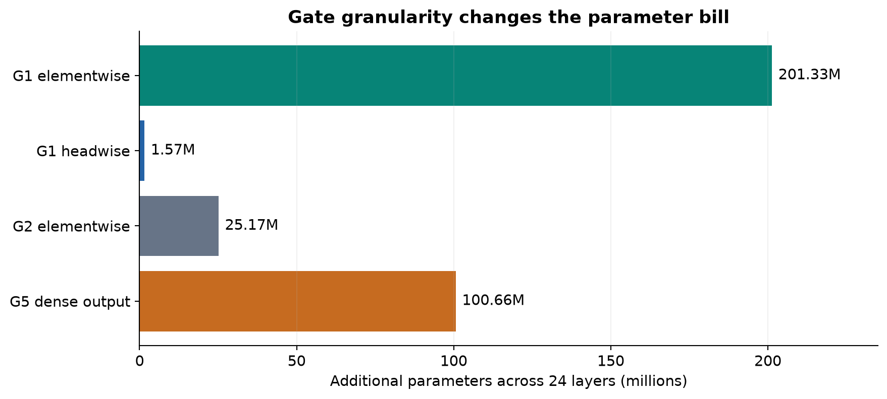
There are two ways a superficial percentage can mislead. The 201M gate is about 1.34% of 15B total parameters, but about 7.9% of the stated 2.54B active parameter count. Neither ratio is automatically the percentage increase in measured step time: different operators have different utilization, communication and bandwidth costs. The paper reports less than 2% wall-time overhead in its experimental setting. That empirical statement should remain attached to that setting.

Temporary activations also depend on granularity. At sequence length 4096, one layer’s unbatched elementwise gate contains $4096\times32\times128=16{,}777{,}216$ scalars. A naively stored BF16 buffer occupies 32 MiB. A headwise gate contains 131,072 scalars, or 0.25 MiB. These are arithmetic examples for a single sequence and layer, not measured peak-memory figures. Fusion, recomputation, batching and sharding change the actual allocation.

Crucially, G1 still computes the ordinary attention-weighted sum over the retained keys and values. Its sigmoid values are generally small positive numbers rather than exact zeros. It introduces neither a token eviction policy nor an asymptotic change to dense attention. A systems benefit would need its own mechanism: for example, a proven sparse execution rule or an independently validated compression scheme. The reported activation sparsity is not such a rule on its own.

The dense-model comparison handles parameter count differently. The authors reduce FFN width when adding gates to keep overall parameter size matched. Those results therefore test a reallocation of a fixed parameter budget as well as a new operation. That is a sensible architecture comparison, but it should be distinguished from simply adding 201M parameters to the same dense network.

6. Reading the main MoE comparison

6.1 What is controlled

The principal MoE sweep uses 400B training tokens. Section 3.1 describes sequence length 4096, batch size 1024 and approximately 100K optimization steps. The learning rate peaks at $2\times10^{-3}$ after a 1K-step warmup and follows a cosine decay to $3\times10^{-5}$. The data includes multilingual, mathematical and general text drawn from a larger training corpus. The paper does not publish a completely reproducible corpus mixture and order.

The scale is large enough that a 0.2-point perplexity change is not merely a toy-model observation. At the same time, many benchmark differences are measured from single reported runs, and the paper’s checklist explicitly states that uncertainty estimates are not reported. This supports taking the broad pattern seriously while remaining cautious about fine rankings separated by a few tenths of a point.

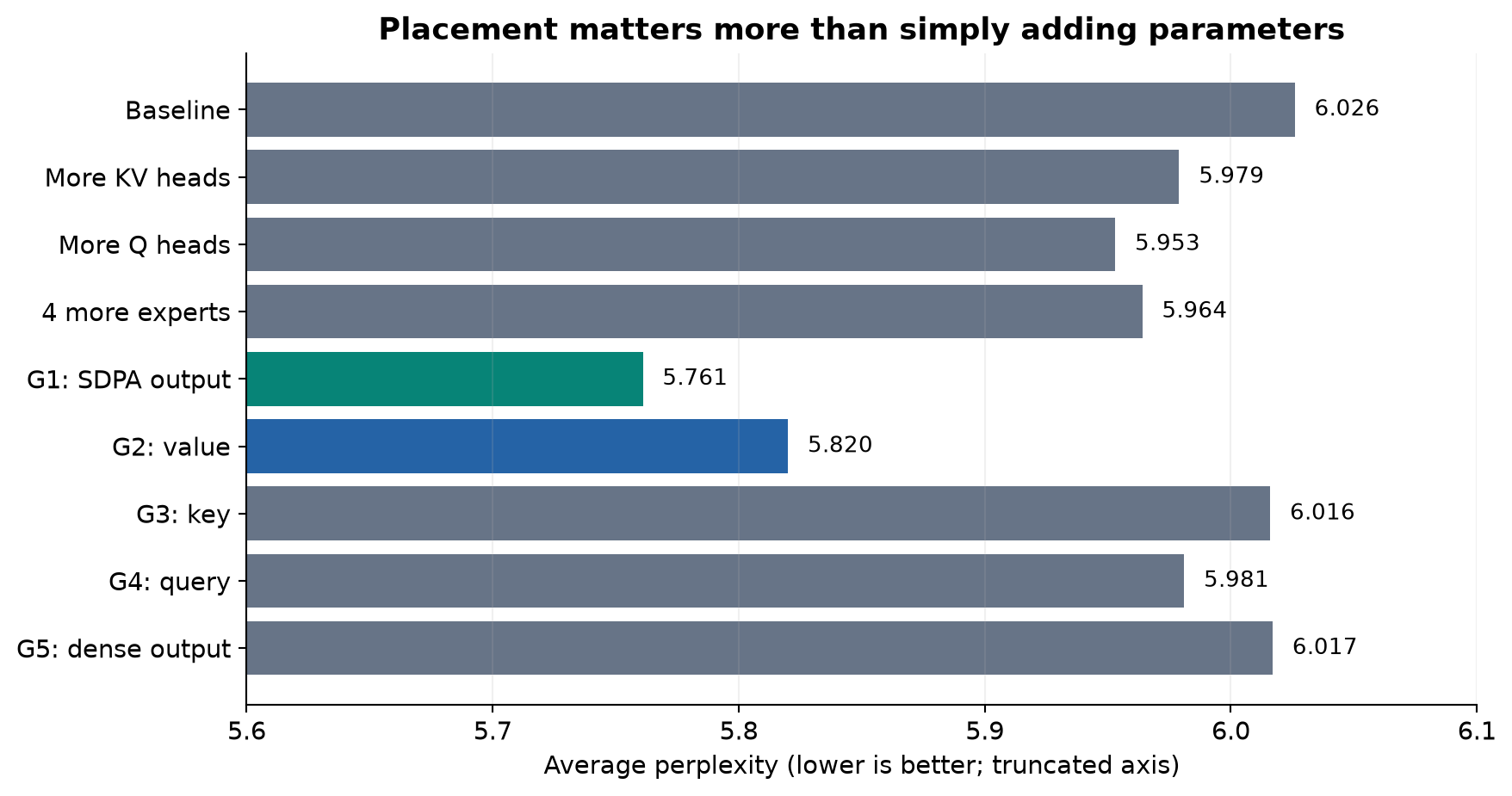
The added-parameter controls are important. Increasing the number of KV heads to eight adds 50M parameters; increasing query heads to 48 adds 201M; adding four experts adds 400M. None matches the best G1 perplexity in Table 1. This rules out the simple explanation that any similar increase in model size would yield the same gain under this recipe. It does not prove that all possible ways to spend an additional parameter or compute budget have been exhausted.

6.2 Placement is a stronger signal than one isolated score

G1 and G2 show clear perplexity gains: 5.761 and 5.820 versus the 6.026 baseline. G3, G4 and G5 give 6.016, 5.981 and 6.017. The result makes the value/output pathway a more compelling intervention point than merely attaching a gate somewhere in attention.

Downstream benchmarks reinforce the usefulness of G1 but also qualify a universal ranking. The G1 elementwise model reports MMLU 60.82 versus 58.79, GSM8K 55.27 versus 52.92, and HellaSwag 74.64 versus 73.07. On C-eval, however, adding four experts reaches 63.19, higher than G1’s 62.20. The additive G1 SiLU variant reports HellaSwag 74.81, slightly above elementwise sigmoid’s 74.64, despite worse perplexity. Different objectives need not select the same architecture.

The headwise G1 variant is especially relevant to a practical design decision. It achieves perplexity 5.792 with about 1.6M extra parameters, close to 5.761 with 201M for the elementwise variant. The additional elementwise parameters buy a modest improvement in this metric. A designer interested in a fixed quality target should compare the two on the actual target workload before treating elementwise granularity as mandatory.

The head-shared G1 variant reaches 5.801, also improving over baseline but with a less favorable diagnostic pattern later. Its average perplexity being relatively close to the other gates illustrates why a large change in an internal statistic does not map mechanically to a large change in every downstream metric.

6.3 What the nonlinear controls establish

Table 3 compares several modifications between the value and output maps. Per-head RMSNorm obtains 5.847 without adding a comparable gate projection. Applying SiLU alone to the attention output gives 5.975. Additive SiLU gives 5.821; an additive identity variant gives 5.882. The strongest sigmoid G1 remains at 5.761.

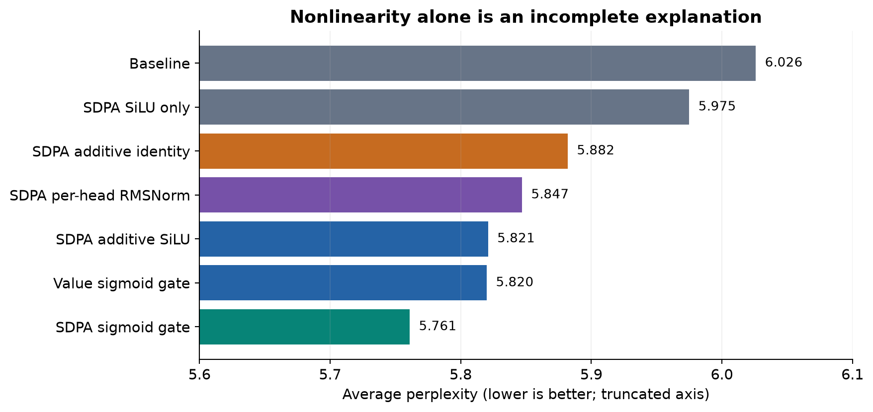
The lesson is narrower than “nonlinearity fixes attention.” Different nonlinear operations produce different results, and a modification without the proposed new nonlinearity can still improve training. RMSNorm changes feature scale and interactions. Additive gates introduce a new input-dependent path. Multiplicative gates condition the existing retrieved content. Each alters both representational behavior and optimization.

The paper’s preferred explanation combines nonlinearity with query-dependent sparse gating, which is more plausible than a one-factor explanation. Even so, a table of architectural variants does not uniquely apportion the performance gain among those mechanisms. The controls are informative contrasts; they are not a full causal decomposition.

7. Sparse activations: what is actually sparse?

7.1 Small gate scores are not a sparse execution schedule

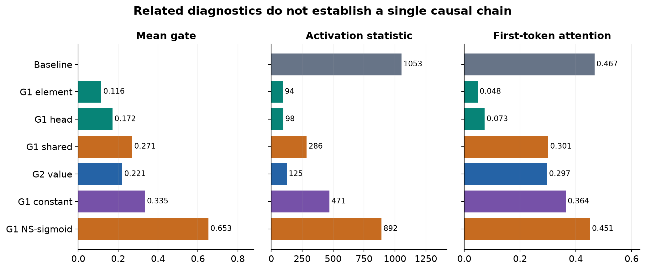
In Table 4, the average G1 elementwise gate is 0.116. Headwise G1 averages 0.172; value gating averages 0.221. The distributions in Figure 3 place substantial mass near zero. Here “sparse” describes soft suppression or the fraction of activations falling below a threshold, rather than exact zeros supplied to a sparse matrix multiplication.

For a scalar logit $u$, $\sigma(u)=1/(1+e^{-u})$ is strictly between zero and one for finite real inputs. A small value may make an output negligible for a particular numerical purpose, but deciding to omit its computation requires a threshold, an error model and an execution strategy. None follows automatically from the gate distribution. Finite-precision underflow is also not the mechanism the paper establishes as the source of its gains.

The distinction is easy to overlook because sparse MoE routing does select a subset of experts. That is a separate mechanism. The word “sparsity” in the gate analysis does not mean that the gate turns this attention layer into an expert router with a fixed top-$k$ execution budget.

7.2 The mean-scaling control prevents an overly strong reading

Appendix A.3 compares three versions of the SDPA output: before gating, after multiplying by a mean gate score, and after applying the actual input-dependent gate. At an absolute threshold of 0.01, the reported average fractions below threshold are 0.03, 0.33 and 0.44. At threshold 0.001, they are 0.003, 0.080 and 0.126.

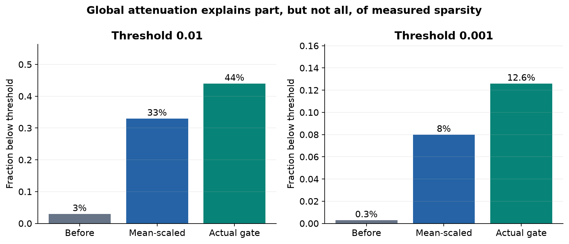
These numbers separate two effects that a histogram alone can mix. If all activations are multiplied by a small constant, many cross a fixed absolute threshold even without any input-dependent selection. The real gate increases the below-threshold fraction further, which is evidence beyond mean attenuation. It is still not a direct measurement of how much semantically irrelevant information has been removed.

For threshold $\tau$, define a measurement on $N$ observed coordinates:

$$S_\tau(y)=\frac{1}{N}\sum_{n=1}^{N}\mathbf 1\{|y_n|<\tau\}.$$

Uniform scaling by a positive $c$ satisfies

$$S_\tau(cy)=S_{\tau/c}(y).$$

Thus changing scale changes the effective threshold. A useful supplementary analysis would normalize by a per-head scale or compare matched output norms. That proposal would answer a different question from the paper’s absolute-threshold statistic and should be labeled accordingly.

7.3 The non-sparse sigmoid ablation changes several things

The paper replaces the sigmoid with

$$\operatorname{NS\text{-}sigmoid}(u) =0.5+0.5\sigma(u).$$

The multiplier is constrained to $(0.5,1)$, preventing strong attenuation. Its model reports mean gate 0.653, perplexity 5.900 and first-token attention 0.451. The original G1 gives 0.116, 5.761 and 0.048. The result supports the usefulness of allowing near-zero outputs.

However, the intervention also changes the mean multiplier, its range and its derivative: the derivative is half that of the ordinary sigmoid at the same logit. It does not vary sparsity while fixing all other factors. Matching the output distribution, testing a shifted logit initialization, or adding a learned global scale would help narrow the explanation.

There is a small source inconsistency worth retaining in a careful reading: Table 4 reports 0.451 for this variant’s first-token attention, while the corresponding Figure 6 legend reports 0.481. This review uses the table value for the table-based chart and does not silently blend the two. The broad contrast with G1’s 0.048 survives either value, but the exact measurement is not fully reconciled by the text.

8. Attention sinks and activation outliers

8.1 Output gating gives a head a near-zero-write option

Consider the scalar headwise case. Multiplying the head output by $\gamma_i^h$ gives

$$z_i^h=\gamma_i^h\sum_j a_{ij}^h v_j =\sum_j\underbrace{\left(\gamma_i^h a_{ij}^h\right)}_{\widetilde a_{ij}^h}v_j.$$

The effective coefficients satisfy

$$\sum_j\widetilde a_{ij}^h=\gamma_i^h.$$

Their total mass can approach zero. This provides a direct way to reduce the head’s contribution without forcing a different competition over token positions. For an elementwise gate, the analogous coefficient mass differs by feature coordinate, so there is no single replacement attention matrix for all value dimensions.

A constructed two-token example makes the distinction concrete. Let the softmax weights be $(0.4,0.6)$ and the values be $(2,1)$ and $(0,3)$. The retrieved vector is $(0.8,2.2)$. A gate $(0.1,0.8)$ yields $(0.08,1.76)$. The first coordinate is strongly attenuated while the second remains substantial. The original probabilities are still $(0.4,0.6)$. The gate did not retroactively change the selection of token positions in this forward computation.

This is why the observed sink reduction is a training result. The architecture gives the network a new way to regulate output; training can then discover different queries, keys and values. One cannot take an arbitrary frozen checkpoint, multiply its existing attention outputs by gates, and infer that its stored attention maps will immediately cease to have sinks.

8.2 The diagnostics show association and useful counterexamples

The baseline maximum-activation summary is 1053, with F-Attn 0.467. G1 elementwise gives 94 and 0.048; headwise G1 gives 98 and 0.073. These are large differences under the paper’s measurement. They make a convincing case that the trained gated models inhabit a different internal regime.

The value-gated model is the more revealing counterexample. Its activation summary is 125, much lower than baseline, but F-Attn remains 0.297. Reducing large activations therefore does not automatically eliminate the first-token attention pattern. Head-shared G1 similarly gives activation summary 286 and F-Attn 0.301. The gate’s placement and independence across heads affect more than overall amplitude.

Appendix A.4 traces large values through FFN outputs and the residual stream. In the plotted baseline, large activations appear around the sixth layer and persist through later residual paths. This observation motivates a connection to normalization and finite-precision behavior. It does not establish that every numerical instability starts at that layer, or that attention output magnitude alone is the root cause.

The paper’s main analysis correctly notes that massive activations are not necessary for attention sinks, as the value-gate example illustrates. A sentence in the related-work discussion uses conflicting wording. The diagnostic counterexample is the better guide: the evidence should not be read as a proven necessary-and-sufficient relationship between the two phenomena.

8.3 Algorithm 2: making the diagnostics interpretable

The following is a proposed measurement protocol for a future controlled comparison, not an additional experiment reported here.

1. Fix an evaluation corpus, context-length distribution, mask policy and averaging convention before comparing architectures.
2. Record gate distributions separately by layer, head and position; preserve more than the global mean.
3. Measure first-token attention and broader sink concentration, separating true first tokens from padding or artificial boundary tokens.
4. Measure pre-gate, post-gate and residual activations, reporting quantiles as well as maxima; document whether maxima are averaged over examples or layers.
5. Compare raw threshold sparsity with mean-scaled and norm-matched controls on the same examples.
6. Relate the diagnostics to task errors, retrieval positions and training events, rather than treating low sink mass as the optimization target itself.
7. Repeat with independent training runs before making claims about causal mediation or small performance differences.

This protocol would make it easier to distinguish a healthier representation from a statistic that looks healthier because its scale changed. It would also expose heterogeneous behavior hidden by a global average: a small number of indispensable sink-like heads could coexist with a low mean.

9. Stability and scaling in the dense experiments

The paper evaluates 1.7B dense architectures with 28 or 48 layers. The 28-layer version uses model width 2048, while the 48-layer version uses width 1536. Both have 16 query heads, eight KV heads and head width 128. These are distinct depth/width configurations, not the same network with 20 identical extra layers appended.

At 28 layers and 400B tokens, perplexity improves from 7.499 to 7.404 at maximum learning rate 0.004. At 3.5T tokens, using maximum learning rate 0.0045 and batch 2048, it improves from 6.180 to 6.130. HumanEval rises from 34.15 to 37.80 in the latter pair, while MMLU rises from 59.10 to 59.61. The small perplexity difference alongside a larger change on a particular benchmark is another reason not to treat one aggregate metric as a complete description.

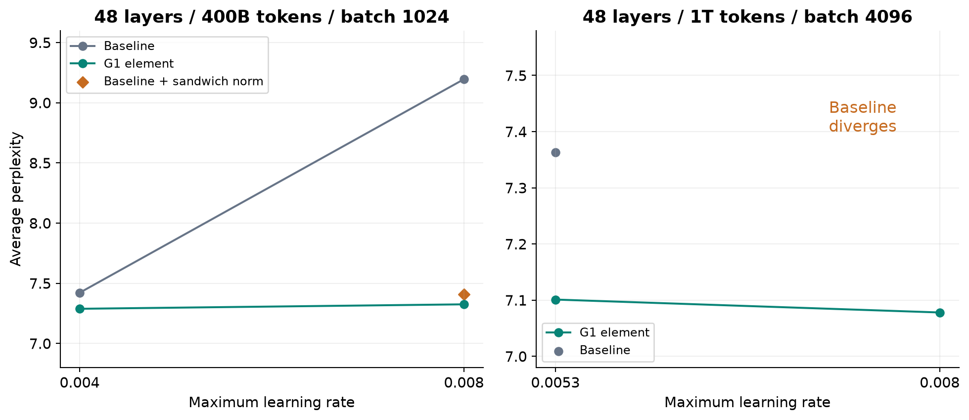
The 48-layer settings sharpen the stability result. With 400B tokens and batch 1024, raising the baseline’s maximum rate from 0.004 to 0.008 worsens perplexity from 7.421 to 9.195. Adding sandwich normalization at 0.008 brings perplexity to 7.407. The elementwise gated model gives 7.288 at 0.004 and 7.325 at 0.008. Thus the gate makes the larger rate usable, but the larger rate does not improve this model’s perplexity in that particular comparison.

Some downstream metrics move differently. In those gated 400B runs, MMLU rises from 52.44 to 54.47 and GSM8K from 32.37 to 36.62 as the maximum rate increases. HumanEval changes from 31.71 to 31.10. Saying “larger learning rates improve all metrics” would erase this tradeoff.

At 1T tokens and batch 4096, the baseline at 0.008 is marked as divergent, whereas the gated model trains and reports perplexity 7.078. At 0.0053, the baseline reports 7.363 and the gated model 7.101. This is stronger evidence that gating expands the usable recipe range under the tested setup. It does not provide a universally safe learning-rate multiplier for a new model, optimizer or precision format.

Appendix A.6 further weakens a one-variable account of stability. Clipping attention and FFN outputs to either 100 or 300 did not resolve the convergence problem at learning rate 0.008. Simply limiting large values was not enough in that experiment. Gating changes the learned map and its gradients throughout training; it is not equivalent to clipping an otherwise unchanged network.

The appropriate engineering inference is to include gating in the architecture/recipe search and then retune the learning rate and batch size. It is not to double the learning rate unconditionally. Useful measurements would include failures across seeds, optimizer-state norms, loss spikes, achieved throughput and final quality at a fixed total training budget. The published evidence justifies that investigation but does not complete it for every deployment setting.

10. Long-context results: preserve the sequence of interventions

The long-context experiment has three stages. First, the dense models are trained on 3.5T tokens. Second, the RoPE base is increased from 10K to 1M, and both models continue training on 32K sequences for an additional 80B tokens. Third, YaRN extends the nominal context to 128K without further training in that extension step. RULER is evaluated before and after the third stage.

The distinction between “no extra training for the final extension” and “no long-context training at all” is essential. These models did receive the additional 80B-token, 32K-context training stage. Omitting that stage would substantially misdescribe the evidence.

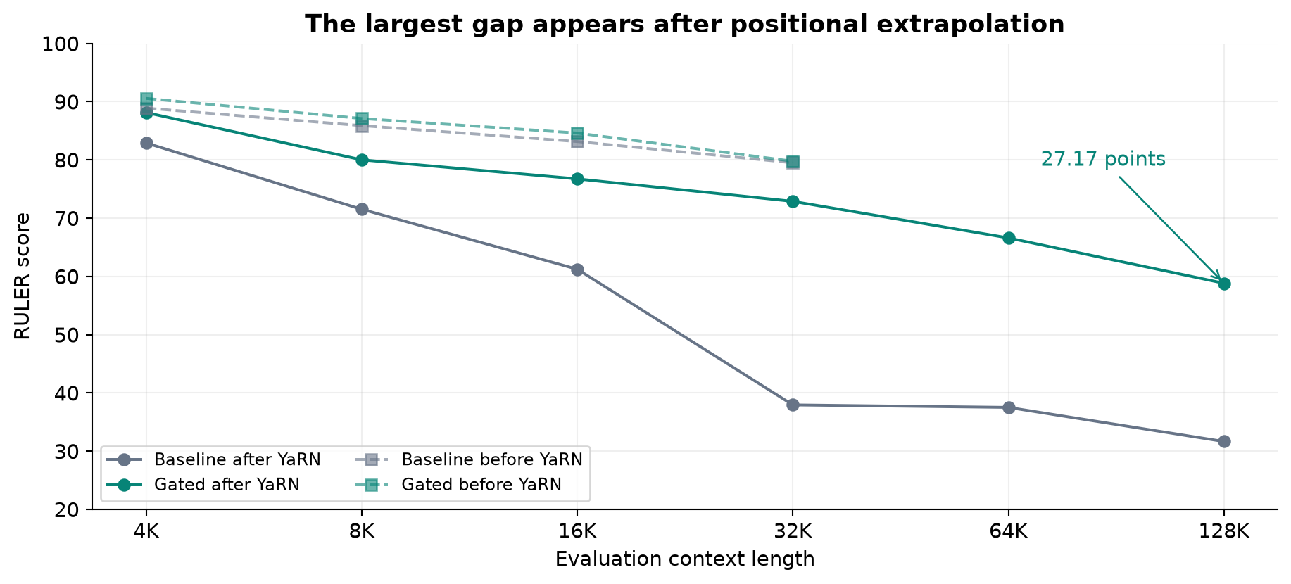
Before YaRN, scores at 32K are 79.50 for baseline and 79.77 for the gate, a difference of only 0.27 points. After YaRN, the same evaluation length gives 37.94 and 72.88, a difference of 34.94 points. The baseline loses 41.56 points at 32K, while the gated model loses 6.89. A difference-in-differences calculation isolates how much more the baseline deteriorates under this intervention:

$$\begin{aligned} \Delta_{\mathrm{extension}} &=(72.88-79.77)-(37.94-79.50)\\ &=34.67\ \text{points}. \end{aligned}$$

At 128K, the extended baseline scores 31.65 and the gated model 58.82, a 27.17-point gap. At 64K the gap is 29.09 points. These are substantial differences within the reported protocol. Yet the small pre-extension gap suggests that the clearest result is robustness to this positional extrapolation, not a blanket claim that attention sinks always destroy long-context retrieval.

The authors hypothesize that a model relying less on sink patterns is less sensitive to changes in positional geometry. That is plausible, but the experiment changes the trained architecture and several associated statistics together. It does not independently manipulate sink strength while holding the rest of the network fixed. The causal mechanism remains less firmly identified than the performance contrast.

A system using this result should also ask whether RULER improvement transfers to its actual task: locating multiple facts, resolving contradictions, generating long code, or interacting with a changing context. The table is not an evaluation of all those activities. A 128K window size, a retrieval score and reliable 128K reasoning are three different properties.

11. Design choices, alternatives and failure boundaries

11.1 Why prefer G1, and when the smaller gate is attractive

G1 has two structural advantages. It conditions the intervention on the current query, and it retains access to separate head coordinates before the dense output projection mixes them. The empirical placement sweep supports both as useful design properties. G2 changes source representations before retrieval; G5 acts after head mixing. Neither gives exactly the same control.

The choice between headwise and elementwise G1 is less absolute. Elementwise gates provide more selective feature modulation, but the headwise variant obtains most of the reported perplexity gain with much smaller parameter overhead. Where attention projection bandwidth, optimizer memory or a fixed model budget matters, that is a serious alternative. The paper does not establish a universal cost-adjusted winner across devices and workloads.

Per-head RMSNorm is another useful comparison. It improves the MoE result without a similarly large input-to-gate projection. It supplies normalization and nonlinearity but does not express the same near-zero-write decision. Sandwich normalization addresses a different location in the residual block and helps the high-rate dense baseline. These alternatives suggest that gate design should be compared jointly with normalization placement, rather than assuming that every model has the same untreated weakness.

11.2 Multiplicative versus additive control

Multiplication makes the retrieved content a prerequisite for the gated output: if a retrieved coordinate is zero, multiplying it still gives zero. An additive path can inject a query-dependent feature even when the retrieved coordinate is zero. That is a different modeling choice, closer to providing another route from the current hidden state.

The paper’s multiplicative sigmoid performs better in average perplexity than its additive SiLU comparison, but that comparison changes both operation and activation. Table 1 also includes multiplicative SiLU, which performs worse than sigmoid on perplexity. Taken together, the comparisons favor the bounded multiplicative option in this setup. They do not prove that additive conditioning is intrinsically inferior in every attention architecture.

A bounded gate can be easier to interpret locally: it says how much of a channel survives. SiLU can be negative and is unbounded above, so its multiplier can reverse or amplify content. Those extra freedoms may affect optimization and calibration. This is a reason the choice is meaningful, not an explanation established by a single accuracy table.

11.3 Training from scratch versus modifying an existing checkpoint

Appendix A.7 is one of the most practically important parts of the paper. Adding output gates during continued pretraining did not remove the existing activation/sink patterns or significantly improve final performance in the reported attempt. The authors suggest that the main benefit is tied to training dynamics from the beginning.

This result should shape deployment expectations. A gate trained alongside all the other projections can change how the network learns to represent irrelevant or unwanted information. Adding it after the network has already developed compensating conventions asks the model to reorganize those conventions. That may require a different adaptation schedule, initialization or objective. The appendix does not give enough evidence to prove that adaptation can never work, but it does reject the assumption that the architectural edit is automatically a checkpoint upgrade.

A useful initialization tradeoff follows directly from the equations. Gates initialized close to one preserve the original output approximately but have a small sigmoid derivative. Gates initialized around one half have a larger derivative but initially shrink the attention contribution. This tradeoff could matter for retrofitting, yet it is a proposed explanation and experimental variable, not a result established by the paper.

11.4 The relationship to linear attention and KV compression

The shared word “gated” can obscure major differences between architectures. In recurrent linear attention, a gate may change how a finite state is forgotten or updated over time. Here G1 modulates the output of an ordinary softmax retrieval. It does not replace the stored sequence of keys and values with a fixed-size recurrent state.

That distinction matters when comparing this paper with Gated Delta Networks or Kimi Linear. A state-update gate governs what information remains available for future queries. A softmax output gate governs what an already computed retrieval writes now. Both are forms of conditional information control, but their memory complexity and failure modes are different.

Likewise, the disappearance of a first-token sink does not authorize dropping that token’s KV entries. A token can matter for some later query even if it receives little attention on the diagnostic corpus. Correctness of a cache policy requires reasoning about the policy and its target workload. The present paper supplies an architectural observation that may motivate such research, not a cache-compression guarantee.

12. Limitations: what the available evidence leaves unresolved

Uncertainty and training variance. The reported runs span substantial scale, but the checklist states that error bars or comparable significance information are not provided. This limits confidence in close rankings, such as differences between two strong gate granularities. It is less damaging to broad contrasts such as a divergent baseline versus a completed gated run, although even failure probability should ideally be measured across seeds.

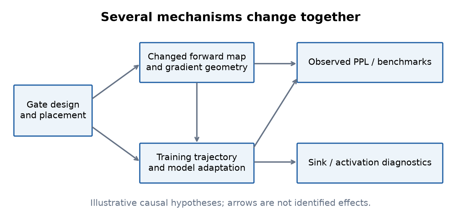
Incomplete isolation of mechanisms. Placement, parameterization, amplitude, nonlinear response, head independence and optimization all change across different variants. The study narrows the plausible explanation substantially but does not identify how much of the gain each mechanism causes. Interpreting correlations among low gate means, smaller activation outliers and lower sink mass as a fully ordered causal chain would go beyond the experiments.

Evaluation coverage. The benchmarks include language modeling, selected reasoning/knowledge tasks and RULER. They do not establish reliability on all production generation tasks, multilingual conditions, post-training recipes or tool-using agents. A gate that helps pretraining can interact differently with later optimization or a different normalization scheme.

Cost reporting. The reported small wall-time overhead is useful but not a complete hardware study. The paper does not provide enough measurements to infer serving latency, peak memory, energy or communication overhead for arbitrary parallel layouts. The dense experiments also exchange FFN width for gate parameters, which changes the budget comparison.

Retrofitting. The negative continued-training result is a real boundary, even though the experiment is not detailed enough to characterize every possible adaptation strategy. This matters for readers with an existing checkpoint and no budget for training from scratch.

Source consistency. Two diagnostics deserve explicit caution. Table 1 reports GSM8K 53.97 for the value-elementwise gate, while Table 4 reports 51.33 for the corresponding row despite matching perplexity and other listed scores. The NS-sigmoid first-token attention discrepancy, 0.451 in Table 4 versus 0.481 in Figure 6, was discussed earlier. Neither inconsistency overturns the main G1 result; both prevent treating every repeated number as a perfectly reconciled measurement. This review uses Table 1 for the primary performance comparison and Table 4 for its diagnostic plot.

Interpretation of averages. A mean gate, mean first-token attention and mean layer maximum omit distributional information. They can hide a few high-impact heads or rare numerical events. The appendix’s layerwise plots improve the picture, but there is no proof that the same patterns characterize every input or deployment regime.

13. Critical Analysis: the empirical result is stronger than a single mechanism story

13.1 What I find most convincing

The placement sweep is the core evidence. Gating the retrieved output consistently stands out relative to gating queries, keys or the dense output under the same broad setup. Parameter-expansion controls make the result more informative than a simple larger-model comparison. The dense experiments then show that the benefit is not confined to one MoE configuration. Together, these support treating query-dependent output control as a useful architectural axis.

The headwise result is also scientifically valuable. A roughly 1.6M-parameter intervention captures much of the performance improvement obtained by the roughly 201M-parameter elementwise gate. This suggests that allowing different heads to choose their contribution strength may be a substantial part of the opportunity. It does not prove that feature-level selectivity is irrelevant; it gives a more focused hypothesis to test.

Finally, the negative appendix results increase the paper’s practical value. Clipping did not reproduce the stability benefit, and adding gates late did not reproduce the training-from-scratch pattern. These observations constrain simple explanations and prevent a reader from treating the successful architectural form as a universally effective patch.

13.2 Three claims deserve narrower wording

First, nonlinearity beyond a low-rank value/output map is a better statement than “the gate removes the rank bottleneck.” The fixed-gate rank bound remains. The improvement comes from an input-dependent family of channel modulations and from its interaction with optimization. That more precise wording is enough to explain why a seemingly small operation can matter.

Second, soft suppression correlated with lower sink mass is more defensible than treating “sparsity” as an independently identified cause. The NS-sigmoid control changes the mean, range and slope; the threshold statistic changes under simple rescaling; the constant-gate result can reflect parameterization. These facts do not invalidate the sparsity hypothesis, but they make it one component of a broader account.

Third, robustness to the tested YaRN extension is the sharpest long-context claim. The large post-extension gap is impressive precisely because the pre-extension gap at 32K is small. Framing the result as resistance to a specific intervention is more useful for future research than a generic statement that sink-free attention is always better at long context.

13.3 Algorithm 3: a future experiment that separates the explanations

The following design is a proposal, not a performed experiment.

1. Select one model architecture and data stream; fix total parameter and training-compute budgets explicitly, and use multiple seeds.
2. Compare no gate, headwise G1 and elementwise G1, retaining a capacity-matched projection control and per-head normalization control.
3. Add a constant-gate parameterization and a dynamic gate whose scores are shuffled across examples or heads, with carefully matched marginal statistics.
4. Add mean- and variance-matched gate controls, documenting the remaining differences in nonlinear response and gradients.
5. Train variants from scratch; separately test several well-specified continued-training initializations rather than mixing these regimes.
6. Evaluate language-model loss, downstream quality, training failure rate and measured cost. Preserve per-layer/head activation and attention distributions.
7. For context extension, cross gate type with positional-extension choice and continued-training budget. Compare pre/post changes on the same evaluation tasks.
8. Analyze whether diagnostic changes predict quality after conditioning on training progress and architecture, and report uncertainty rather than only the best run.

Shuffling scores is not a perfect intervention: it can itself introduce distribution mismatch. Likewise, matching gate means does not match the entire gradient field. The purpose is not to claim that a single additional ablation will solve causality, but to reduce the most obvious confounds with a coordinated set of comparisons.

13.4 A decision-oriented interpretation

For a new pretraining project, the paper supports evaluating G1 gating early, including a headwise baseline, and searching its interaction with learning rate and normalization. For an existing checkpoint, the evidence supports caution about expected gains from a quick architectural retrofit. For an inference system, it supports no immediate claim of lower KV memory or fewer attention FLOPs.

The broader idea is that token selection and write strength need not share one normalization constraint. An attention layer can select useful context while separately deciding how much of each retrieved channel to add. This separation is a plausible reason the intervention travels across settings. Its precise quantitative benefit still depends on the learned network, not only the elegance of the formula.

14. Conclusion

Gated Attention makes a small change at a consequential location: it multiplies each softmax head’s retrieved output by a query-dependent gate before mixing heads. The paper provides substantial empirical evidence that this improves its tested pretraining configurations, changes activation and sink patterns, and makes the resulting models more robust to a specific long-context extrapolation.

The careful interpretation is also the more actionable one. The gate introduces conditional channel control, retains a per-head rank bound, adds computation, and does not by itself compress the KV cache. Its strongest evidence concerns jointly trained architectures. Its internal diagnostics motivate hypotheses rather than closing the causal explanation.

For my own reading, the most useful takeaway is to treat how much a head writes as a first-class architectural choice. The best next comparison is not merely another larger model, but a cost-aware study of headwise control, featurewise control, normalization and training dynamics under the same budget.

15. Sources and figure provenance

1. Qiu et al., Gated Attention for Large Language Models: Non-linearity, Sparsity, and Attention-Sink-Free, NeurIPS 2025. The 27-page proceedings PDF is the primary source for equations, experiment settings, Tables 1–7 and Appendices A.1–A.9 discussed here.
2. arXiv:2505.06708, bibliographic record and original May 2025 version. This review does not substitute the shorter arXiv PDF for the expanded conference document.
3. Official author resource, a navigation link for readers seeking released materials.

Figures 1 and 9 are original diagrams; Figure 2 derives parameter costs. Figures 3–8 redraw reported values from Tables 1–5 and Appendix A.3. Proposed experiments and illustrative calculations are this review’s analysis, not additional author results.