Progressive Point Matching: Dense Credit for Long-Horizon Language Model RL

Date: September 22, 2026
Author: Zhongzhu Zhou
Paper reviewed: Long-Horizon Language Model Reinforcement Learning via Progressive Point Matching
Paper authors: Preston Fu, Kevin Frans, Oleh Rybkin, Sergey Levine, Aviral Kumar
Version: arXiv:2609.07303v1, September 7, 2026
This review covers the 38-page paper, including Appendices A–D.
Resources: Author page · Official code resource

1. The useful idea, and the boundary of the claim

Suppose a model completes nine useful steps in a mathematical solution and fails on the tenth. An outcome-only verifier gives the same zero reward to this trajectory as to an attempt that accomplished nothing. That is a particularly expensive loss of information when generating a trajectory takes thousands of tokens. Progressive Point Matching, or PPM, asks whether a reference solution can provide intermediate landmarks without forcing the learner to reproduce the reference word for word.

The proposed answer has three parts. First, express a reference solution as reasoning points: useful mathematical statements or intermediate results. Second, score the cumulative points reached by each generated prefix and reward increases in that score. Third, apply shortcutting: a later achievement can make an earlier reference step unnecessary, so the model can receive its credit without explicitly taking that step. In the ideal formulation, reaching the final goal awards all remaining reference credit.

These pieces address different problems. Intermediate points create feedback before complete success becomes common. Segment rewards reduce the indiscriminate broadcasting of one score over an entire response. Shortcutting prevents a model that discovers a shorter valid solution from losing to a model that follows a longer reference route. None of these benefits requires a reference solution to appear in the policy’s input during ordinary rollouts; privileged information is used by the reward construction.

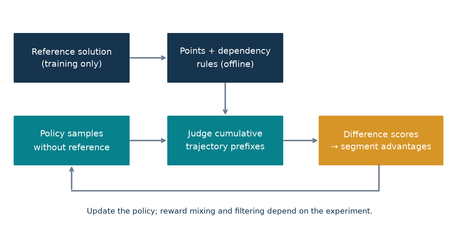
The strongest empirical evidence is the controlled horizon study and the selected near-zero-reward math setting. The paper also contains a valuable qualification: PPM is not the best method on every benchmark or under every token budget. On the Polaris-trained model, GRPO has higher AIME25 pass@1 than PPM. On POPE-hard, training PPM at 4K tokens gives better pass@8 at 16K than training it at 8K, while the 8K-trained model has slightly better pass@1. The appropriate conclusion is improved access to useful training signal in some hard regimes, not universal domination.

Three levels of evidence should remain separate throughout this review:

Level	What it establishes	What it does not establish
Ideal reasoning graph	A conditional optimal-policy equivalence	Equality of all policy rankings or of all gradients
Stylized gradient model	How projected SNR scales with graph structure	An unconditional end-to-end compute scaling law
LLM experiments	Reported gains under specified models, judges and budgets	Reliability on arbitrary long-running agents

All experimental numbers below come from the paper. Original diagrams and numerical examples are labeled as illustrations; they are not additional model-training results.

2. Prerequisites: why a long answer is hard to reinforce

2.1 Tokens, trajectories and policy gradients

A language model policy generates token $x_t$ conditional on its prefix. For a fixed prompt, the probability of a response is a product of conditional probabilities:

$$p_\theta(x_{1:T})=\prod_{t=1}^{T}\pi_\theta(x_t\mid x_{<t}).$$

Let $R(x)$ be a verifiable final-answer reward. Differentiating its expectation and applying the log-derivative identity gives

$$\begin{aligned} J(\theta)&=\sum_x p_\theta(x)R(x),\\ \nabla J(\theta)&=\sum_x p_\theta(x)R(x)\nabla\log p_\theta(x),\\ &=\mathbb E_x\!\left[R(x)\sum_{t=1}^{T}\nabla\log\pi_\theta(x_t\mid x_{<t})\right]. \end{aligned}$$

The estimator is simple, but one scalar multiplies contributions from all generated tokens. A correct final answer may follow useful work, redundant work, a lucky guess, or a mixture of these. Conversely, a failed answer may contain valuable intermediate reasoning. Outcome reward alone does not distinguish them.

Subtracting a suitable baseline reduces variance without changing the intended gradient in the standard setting. It cannot manufacture distinctions inside a group in which every trajectory receives the same zero reward. With a group of $G$ samples, even getting one success can be difficult. If a complete trajectory succeeds with probability $q$, the probability of at least one successful sample is

$$P_{\mathrm{nonzero}}=1-(1-q)^G.$$

For an illustrative chain with per-step success $p=0.7$ and 20 necessary steps, $q=p^{20}\approx0.000798$. A group of 16 then has only about a 1.27% chance of containing a success. This calculation assumes independent necessary steps and is not an estimate for the actual Qwen runs. It shows why merely increasing group size can become costly.

2.2 Progress is different from local correctness

A process reward commonly checks whether a step is logically correct. PPM instead asks whether a prefix has reached a useful reference point. Those criteria overlap but are not identical. Writing a true identity that has no connection to the problem can be locally correct and make no progress. Reaching a useful intermediate numerical result by a different derivation can make progress without matching the reference’s wording.

There is also an uncomfortable converse: the PPM grading prompt in Appendix D instructs the judge to assess whether the target result appears, rather than whether the derivation that produced it is sound. This deliberately separates point reachability from proof verification. It may help detect useful results after imperfect reasoning, but it creates a need to distinguish a supported result from a lucky unsupported assertion. A strong final verifier is especially important in that setting.

2.3 A compact notation guide

Symbol	Meaning in this review
$s_k$	Set of points reached by prefix through segment $k$
$s^{\mathrm{ref}}$	Reference points, including a final goal $g$
$N$	Number of reference points used in the reward definition
$\phi(s)$	Count of reference points credited at state $s$
$m_k$	Normalized prefix score $\phi(s_k)/N$
$K$	Number of trajectory segments; often four in the paper
$r_k$	Increment in prefix score
$n$	Task horizon in the Appendix A model
$C,D$	Reached-point count and reached cumulative depth in Appendix A

Using $N$ for reference-cardinality and $n$ for the theoretical horizon avoids confusing a mathematical reasoning dependency count with a token count. A 4K response may have four scoring chunks and many more or fewer than four actual reasoning points.

3. From a reference solution to a progress measure

3.1 Reasoning states and their strong abstraction

The paper treats an intermediate result as a sufficient statistic for later reasoning. If two different prefixes establish the same lemma, future reasoning can use the lemma without needing the same proof text. A state is the set of available points, and an action adds points to that set. In this abstraction, progress is monotone: a later mistaken sentence does not erase a previously established lemma.

This is a modeling choice. An actual autoregressive model conditions on the complete textual prefix, including mistakes, confusing notation and distracting statements. Two prefixes with the same abstract points need not induce the same continuation distribution. The abstraction is useful for reward design, but its adequacy must be tested rather than assumed from the fact that an LLM consumes text sequentially.

For reference points $s^{\mathrm{ref}}=\{s_1^{\mathrm{ref}},\ldots,s_N^{\mathrm{ref}}=g\}$, the ideal count is

$$\phi(s)=\sum_{i=1}^{N}\mathbf 1\{s_i^{\mathrm{ref}}\in s\},\qquad 0\leq\phi(s)\leq N.$$

Here membership includes the shortcutting closure defined next. Dividing by $N$ makes different problems’ maximum progress comparable. This scaling does not change a single problem’s optimal policies, although cross-problem scaling matters once gradients are combined across a heterogeneous dataset.

3.2 Why shortcutting is essential

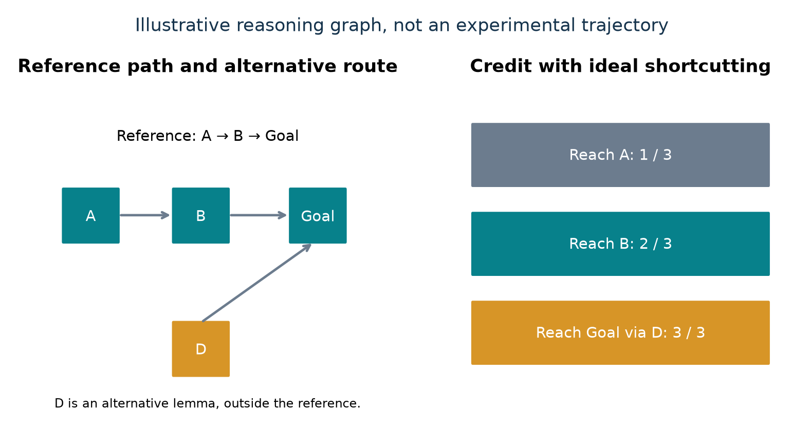
Imagine a reference route $A\rightarrow B\rightarrow g$. Another valid route reaches an alternative lemma $D$ and then the goal. Literal reference matching could give the successful alternative only one point, while an unfinished $A,B$ prefix receives two. The reward would then prefer more reference overlap over solving the problem.

Shortcutting gives credit to obsolete prerequisites once the relevant downstream points have been reached. In the ideal graph, reaching $g$ closes all reference points. Importantly, this is an accounting rule for the reward. It does not claim the model literally generated the missing lemmas, nor does it reveal those lemmas to the policy.

With segment boundaries $0,1,\ldots,K$, define

$$m_k=\frac{\phi(s_k)}{N},\qquad m_0=0,\qquad r_k=m_k-m_{k-1}.$$

A reviewer example has prefix scores $0,0.25,0.50,0.50,1$. Its segment rewards are $0.25,0.25,0,0.50$. Repeating a fact in the third segment earns nothing new; reaching the goal in the fourth grants the remaining credit. An unfinished route with terminal score $0.75$ still supplies a learning signal but cannot attain the successful route’s total of one under the ideal assumptions.

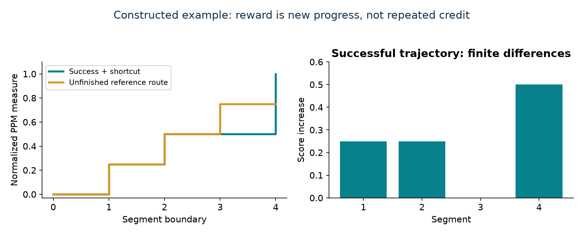
The practical judge scores full prefixes, not isolated chunks. This preserves definitions and notation established earlier. It costs more input tokens, but avoids asking a judge to evaluate an algebraic step without the quantities on which it depends. Perfect monotonicity belongs to the abstract set construction; a noisy judge’s independent scores are not automatically monotone.

4. What the optimality proposition actually proves

4.1 The telescoping argument

Summing finite differences cancels every intermediate score:

$$\begin{aligned} \sum_{k=1}^{K}r_k &=(m_1-m_0)+(m_2-m_1)+\cdots+(m_K-m_{K-1})\\ &=m_K-m_0=m_K. \end{aligned}$$

Suppose that the goal is one of the reference points, that successful goal-reaching receives all reference credit, and that an admissible policy reaches the goal almost surely. Every trajectory’s normalized return lies in $[0,1]$. A policy has expected return one exactly when its terminal progress equals one almost surely. Because full credit requires the goal point, this is exactly the set of policies with success probability one. Thus the sets of optimal policies under ideal PPM and binary outcome reward coincide. This is the substance of Proposition 4.1.

The result does not say $\mathbb E[m_K]=\mathbb E[R]$ for all policies. Unsuccessful but partially productive trajectories explicitly receive positive PPM reward. Nor does the proposition imply that every finite policy-gradient run reaches a global optimum. A statement about optimal policies in an ideal MDP is different from a convergence theorem for a neural optimizer with approximate judges.

4.2 Why the almost-sure reachability assumption matters

Consider a reviewer-constructed problem with ten reference points including the goal. Policy A succeeds with probability 0.6 and otherwise gets no points. Policy B never succeeds but always reaches nine reference points. Then

$$\begin{array}{c|cc} &\mathbb E[R]&\mathbb E[m_K]\\\hline A&0.6&0.6\\ B&0&0.9 \end{array}$$

If these are the only feasible policies, maximizing partial credit selects B, whereas maximizing success selects A. The example does not refute Proposition 4.1: its hypothesis is absent. If a feasible policy C always solves the task, C attains one under both objectives and wins. The example instead explains why the hypothesis is operationally important when the training token budget makes complete success impossible or when the model class is too restricted.

Even with an ideal successful policy somewhere in the class, PPM can reorder imperfect policies along the optimization path. That reordering is the intended source of extra signal. Calling the method “unbiased” should therefore be read in the paper’s qualified, optimal-policy sense, not as a guarantee that an arbitrary PPM gradient is an unbiased estimator of the outcome-only gradient.

4.3 Terminal potentials and discounting

For unnormalized counts, let $R(s)=\mathbf 1\{g\in s\}$ and $\Phi(s)=\phi(s)-R(s)$. At nonterminal states with $R(s)=0$,

$$\begin{aligned} R(s')+\Phi(s')-\Phi(s) &=R(s')+\phi(s')-R(s')-\phi(s)\\ &=\phi(s')-\phi(s). \end{aligned}$$

This resembles potential-based reward shaping with discount factor one. The crucial distinction, explicitly noted in the paper’s footnote, is that unsuccessful terminal states retain a nonzero potential. Consequently, partial terminal progress affects the objective. One cannot import a more general potential-shaping invariance result while silently changing its terminal conditions.

Discounting also changes the cancellation. For $\gamma<1$,

$$\sum_{k=1}^{K}\gamma^{k-1}(m_k-m_{k-1}) =\gamma^{K-1}m_K+(1-\gamma)\sum_{k=1}^{K-1}\gamma^{k-1}m_k.$$

Earlier progress now has extra weight, and the return depends on the path. This identity follows by shifting the index of the second sum and collecting each $m_k$ term. It is useful when considering token costs, latency penalties or early termination: those extensions need their own objective analysis. They are not already covered by the undiscounted proposition.

5. Why localized credit can have better signal-to-noise

5.1 Assumptions before asymptotics

Appendix A analyzes a stylized graph with $n$ reasoning points. Each point $v$ has a prerequisite set $P_v$ containing itself. Independent Bernoulli variables $B_v$ with fixed success probability $p$ represent successful local reasoning. A point is reached only if all its prerequisites succeed:

$$I_v=\prod_{j\in P_v}B_j,\qquad d_v=|P_v|.$$

Rather than analyze the full parameter-vector gradient, the authors project a token/turn score onto a fixed direction, obtaining $x_v$. Their moment assumptions are

$$\mathbb E[x_v]=0,\quad\mathbb E[B_vx_v]=\mu\ne0,\quad \mathbb E[B_vx_v^2]=\lambda,\quad\mathbb E[x_v^2]=\eta.$$

Pairs $(B_v,x_v)$ are independent across points and these constants do not change with horizon. Real LLM steps share parameters, context, difficulty and failure modes, so this is an explanatory model of credit assignment rather than a literal model of every transformer gradient.

The three projected estimators are

$$Y_1=I_g\sum_vx_v,\qquad Y_2=\frac{1}{n}\left(\sum_v I_v\right)\left(\sum_vx_v\right),\qquad Y_3=\frac{1}{n}\sum_vI_vx_v.$$

They correspond to sparse final reward, trajectory-level partial credit, and local partial credit. In $Y_2$, a useful point multiplies every score, including unrelated ones. In $Y_3$, that cross-contamination is removed in the idealized estimator. This is a more precise intuition than simply saying that “dense rewards are better.”

5.2 Deriving the sparse-reward penalty

Define $\mathrm{SNR}(Y)=|\mathbb E[Y]|/\sqrt{\mathrm{Var}(Y)}$. When success requires all $n$ Bernoulli events, independence gives $\mathbb E[I_gx_v]=\mu p^{n-1}$. Summing over $v$ yields

$$\mathbb E[Y_1]=n\mu p^{n-1}.$$

The square contains $n$ diagonal terms and $n(n-1)$ ordered off-diagonal terms. Their expectations are respectively $\lambda p^{n-1}$ and $\mu^2p^{n-2}$. Therefore

$$\begin{aligned} \mathrm{Var}(Y_1) &=n\lambda p^{n-1}+n(n-1)\mu^2p^{n-2} -n^2\mu^2p^{2n-2},\\ \mathrm{SNR}(Y_1)^2&=\Theta(p^n),\\ \mathrm{SNR}(Y_1)&=\Theta(p^{n/2}). \end{aligned}$$

For an average of $M$ independent samples, the variance falls by $M$ and SNR grows by $\sqrt M$. Holding SNR fixed in this model thus demands a sample count scaling like $p^{-n}$, up to the constants implicit in the asymptotics. That is the theoretical origin of the exponential horizon concern. It is not a statement that every RL dataset’s training time follows precisely this curve.

5.3 The graph enters through progress variance

Let $C=\sum_vI_v$ count reached points. For local credit, Appendix A derives

$$\mathbb E[Y_3]=\frac{\mu}{pn}\mathbb E[C],$$

and, separating diagonal from paired contributions,

$$\mathrm{Var}(Y_3) =\frac{\mu^2\mathrm{Var}(C)+(p\lambda-\mu^2)\mathbb E[C]}{p^2n^2}.$$

Canceling the common factor from mean and standard deviation gives

$$\mathrm{SNR}(Y_3)= \frac{\mathbb E[C]}{\sqrt{\mathrm{Var}(C)+\kappa\mathbb E[C]}},\qquad \kappa=\frac{p\lambda}{\mu^2}-1\geq0.$$

The nonnegativity follows from Cauchy–Schwarz: $\mu^2\leq p\lambda$. The formula makes the important variable visible: not merely the expected amount of progress, but how correlated and variable that progress is across trajectories.

For independent tasks, $C$ is binomial, so $\mathbb E[C]=np$ and $\mathrm{Var}(C)=np(1-p)$. The local estimator’s SNR grows as $\Theta(\sqrt n)$. For a sequential chain, reaching a later point requires all earlier successes. The sums $\sum_{v=1}^np^v$ and the relevant second moments stay bounded as $n$ grows at fixed $p$, producing $\Theta(1)$ SNR instead. Both are much better than the sparse estimator’s exponential decay, but the benefits differ with dependency structure.

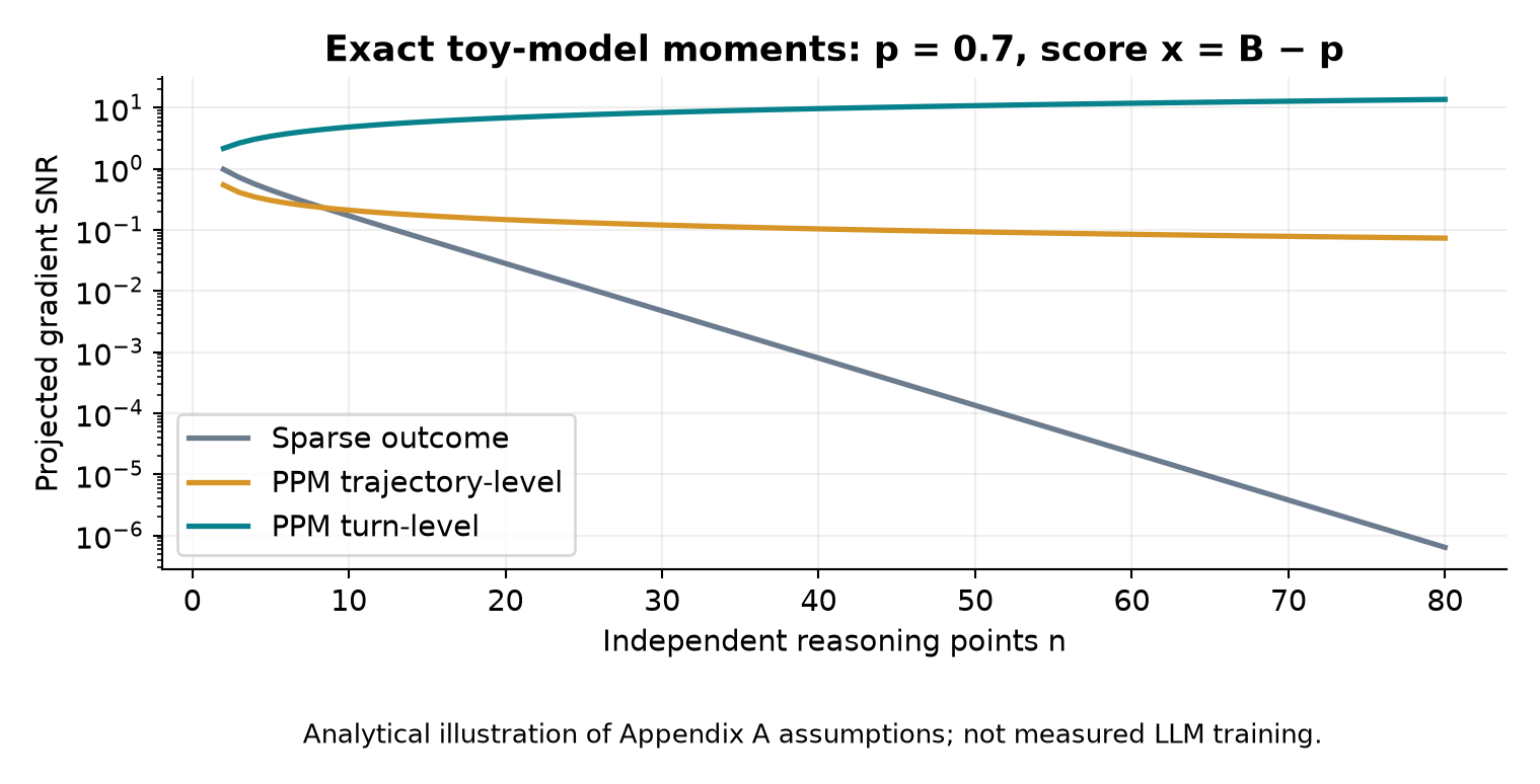
Trajectory-level PPM has $\Theta(n^{-1/2})$ SNR under the regularity assumptions in Proposition A.3. The general bounds are weaker. Appendix A also constructs branching graphs where progress arrives in correlated bursts; turn-level SNR can decline as $\Omega(n^{-1/2})$ in the general worst case, while an additional moment condition yields an $\Omega(1/\log n)$ lower bound. These qualifications prevent extrapolating the favorable independent-task rate to every agent workflow.

There is a reporting detail worth checking in a future paper revision: the prose following Proposition A.7 says that one dandelion setting gives the same $n^{-1/2}$ SNR for $Y_2$ and $Y_3$, whereas Proposition A.10 subsequently states a growing lower bound on their ratio. These statements cannot both be used without clarification under an identical set of assumptions. The exact moment formulas above and the separately described independent/chain cases are the more useful basis for understanding this review’s figure.

6. A training recipe, with theory separated from experiment

6.1 Algorithm 1: ideal progressive point matching

The following pseudocode spells out the conceptual procedure. It intentionally names the advantage mapping rather than pretending all possible PPO/GRPO mappings are equivalent.

Algorithm 1. Ideal PPM reward construction and policy update
Input: policy theta; problems with reference solutions; segment rule
1. Extract reference points and prerequisite/obsoletion relations.
2. For each training iteration, sample from the current policy.
3. Split every trajectory into K segments c[1], ..., c[K].
4. Initialize credited points S = empty and m[0] = 0.
5. For k = 1, ..., K:
     a. Judge points reached by prefix c[1:k].
     b. Form the reached set and apply shortcutting closure.
     c. Set m[k] = credited reference points / total points.
     d. Set r[k] = m[k] - m[k-1].
6. Map segment rewards to token advantages using the chosen rule.
7. Apply the policy-gradient update on generated tokens only.
8. Repeat; evaluate with final outcome success, not PPM score alone.

Steps 5a–5b have ideal set semantics here. The published experiments use LLM grading prompts and inferred graphs, so judge consistency and closure quality are empirical issues. The paper’s Algorithm 1 leaves the function from segment rewards to token advantages abstract. The manuscript should be read with Appendix B to understand the concrete experimental recipe.

6.2 What the experimental recipe adds

The default setup uses synchronous on-policy training: one sampling step followed by one training step. Table 3 reports temperature 1.0, clipping thresholds 0.20/0.28, learning rate $3\times10^{-6}$, 150 steps, 16 trajectories per prompt, eight prompts per batch, and a total batch of 128. Runs use v5e-32 TPU pods and reportedly last 12–24 hours. Those are reported settings, not hardware used for this review.

Several decisions materially alter the basic story:

• Outcome mixing. For the ordinary experimental recipe, the final outcome reward is added to every segment’s method-specific reward before advantage computation. That encourages answer formatting and completion within budget. This is not merely the telescoping PPM objective in Section 4.
• Group centering without standard-deviation division. PPM benefits from subtracting the group mean while omitting the usual division by group standard deviation. Small absolute differences are not automatically amplified to unit scale.
• Truncation masking. Trajectories cut off by the training token budget are masked out of the loss to reduce length pressure. This changes which generated data actually contributes to an update.
• Fixed-budget chunks. Without natural turns, four chunks are defined relative to the training budget, rather than relative to each sampled response’s actual length. Empty chunks receive zero progress reward for advantage calculations.

There are experiment-specific exceptions. Polaris RL uses learning rate $10^{-6}$. In POPE-hard PPM, Appendix B.2 specifies 16 prompts per batch, a KL penalty coefficient of 0.002 using the k3 estimator, and PPM reward alone, without adding outcome reward. It would be wrong to describe every result as using a single uniform reward mixture or as universally having no KL penalty.

To see the scale of outcome mixing, write an illustrative mixed segment reward as $\tilde r_k=r_k+R$. Then

$$\sum_{k=1}^{K}\tilde r_k=m_K+KR.$$

This algebra describes the sum before group centering, masking and token weighting. It does not by itself recover the full optimization objective. It does show that the number of segments can affect the relative strength of final success unless the weighting is adjusted. Four chunks are consequently part of the experimental configuration, not an innocuous visualization choice.

6.3 Algorithm 2: paper-level accounting for a batch

Algorithm 2. Track the experimental reward recipe
Input: a batch, K budget-defined chunks, reward configuration
1. Generate each response and retain its true termination status.
2. Score cumulative prefixes against the per-problem reference.
3. Difference adjacent scores to obtain each segment's progress.
4. If this experiment mixes outcomes, add final reward per segment.
5. Center rewards within the specified GRPO grouping.
6. Apply the configured advantage-to-token mapping.
7. Apply truncation and probability-mismatch masks as specified.
8. Report kept trajectories, train tokens, judge usage and outcomes.

This is an explanatory accounting checklist, not a claim that the paper specifies every grouping detail in this exact order. In particular, reward-to-go versus immediate local credit must not be silently interchanged. The ideal $Y_3$ derivation motivates localization under its assumptions; it is not a blanket proof that any token advantage heuristic optimizes the same full trajectory objective.

7. Controlled experiments: where horizon is the variable

7.1 Independent versus sequential subtasks

Multi-Countdown requires solving $n$ independent arithmetic problems, with a final success only if all are correct. It uses Qwen3-1.7B, with 512 tokens per turn. Matrix Manipulation requires applying operations sequentially to a matrix, using Qwen3-4B-Instruct-2507 with thinking disabled. Here an earlier mistake can prevent later valid states from being reached. These two tasks deliberately approximate opposite graph structures.

Figure 4 of the paper reports growing training-token advantages for turn-level PPM as Multi-Countdown horizon increases: the annotated speedups are 1.8×, 3.5×, 8.7× and 19.7× for $n=2,4,6,8$. These are not general inference speedups or wall-clock speedups. They concern reaching the specified success target during training in this controlled task. Matrix Manipulation also improves, but its dependence structure yields a different scaling pattern, consistent with the theoretical distinction between independent and sequential progress.

The paper intentionally chooses easy-to-verify intermediate states to isolate the effect of reward assignment. The semantic-judge problem enters more strongly in the next experiment. This separation is a strength: otherwise an apparent horizon effect could simply reflect the judge becoming worse as responses grow.

7.2 GSM-Infinite: a less artificial credit interface

GSM-Infinite generates math questions from relational graphs. The authors construct fixed-complexity datasets at $n=8,16,24$, each with 5,000 prompts, and set 40% of edges to be task-relevant while the rest are distractors. They train Qwen3-1.7B without thinking mode at a 4K budget. The reference graph is rendered into textual points, and a Gemini judge scores prefixes.

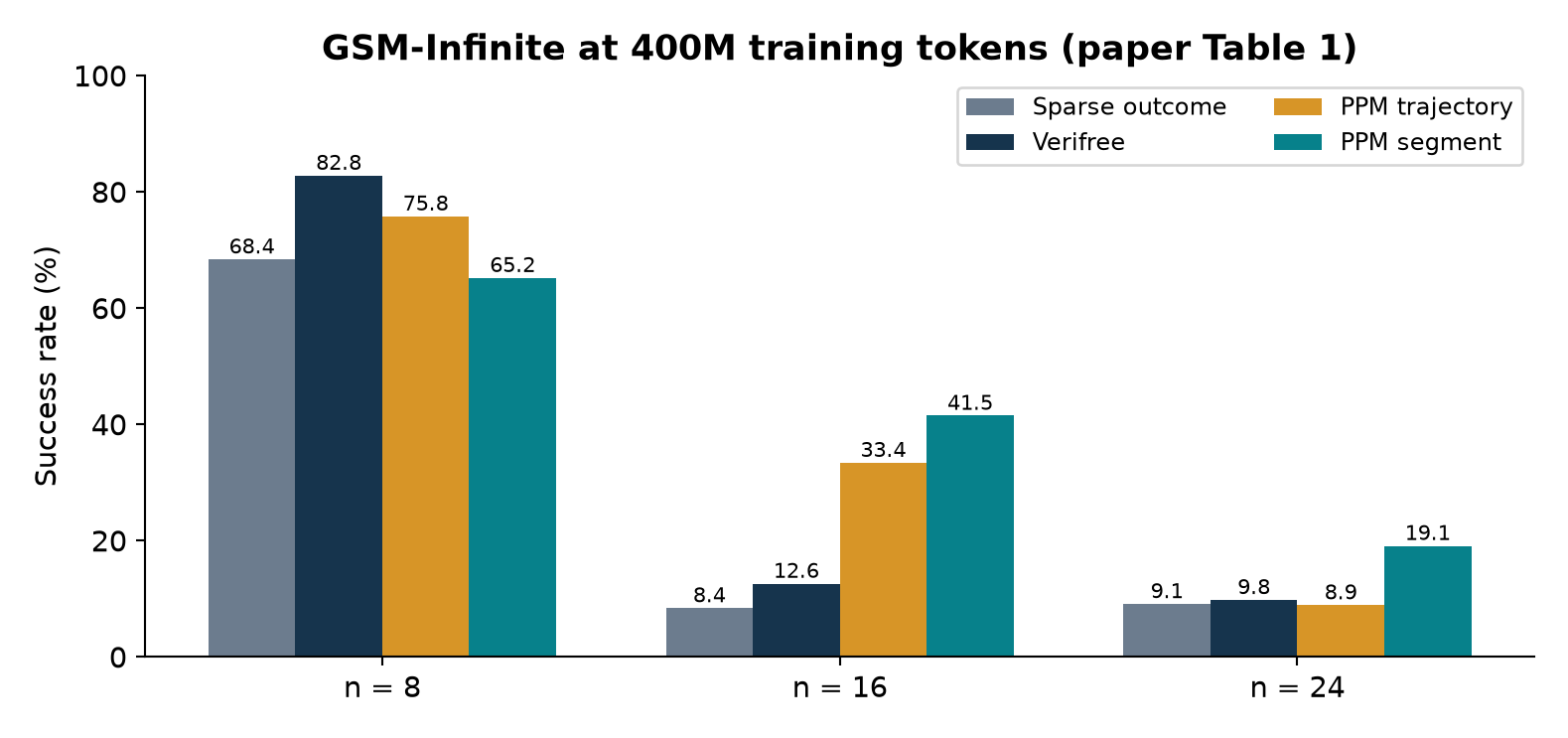
Method	$n=8$	$n=16$	$n=24$
Base model	13.4%	5.6%	5.6%
Sparse outcome	68.4%	8.4%	9.1%
Verifree	82.8%	12.6%	9.8%
OPSD	28.3%	10.2%	7.8%
Process reward	32.9%	7.5%	8.0%
PPM trajectory	75.8%	33.4%	8.9%
PPM segment	65.2%	41.5%	19.1%

At $n=24$, segment PPM gains 10.0 percentage points over sparse outcome reward, roughly 2.10× its success rate. It also more than doubles trajectory PPM’s 8.9%. At $n=8$, however, Verifree leads and segment PPM is below sparse outcome training. The value of localization grows with this benchmark’s horizon; the table does not support making it a default winner on easy tasks.

The process baseline is also a bundle of changes: local correctness instead of progress, no shortcutting, and independent chunk grading instead of full-prefix finite differences. Its weakness establishes a contrast between recipes, but does not isolate exactly which of those differences is causal. A factorial experiment would be needed to do that.

8. Ablations: the practical method is more than a new score

Table 4 holds the GSM-Infinite horizon at 24 and compares recipe changes at 400M training tokens. The full PPM recipe reaches 19.1%; removing outcome reward drops it to 6.3%, adding standard-deviation normalization drops it to 7.1%, using trajectory-length chunks gives 14.8%, and removing the length filter gives 17.1%. Sparse outcome training reaches 9.1%.

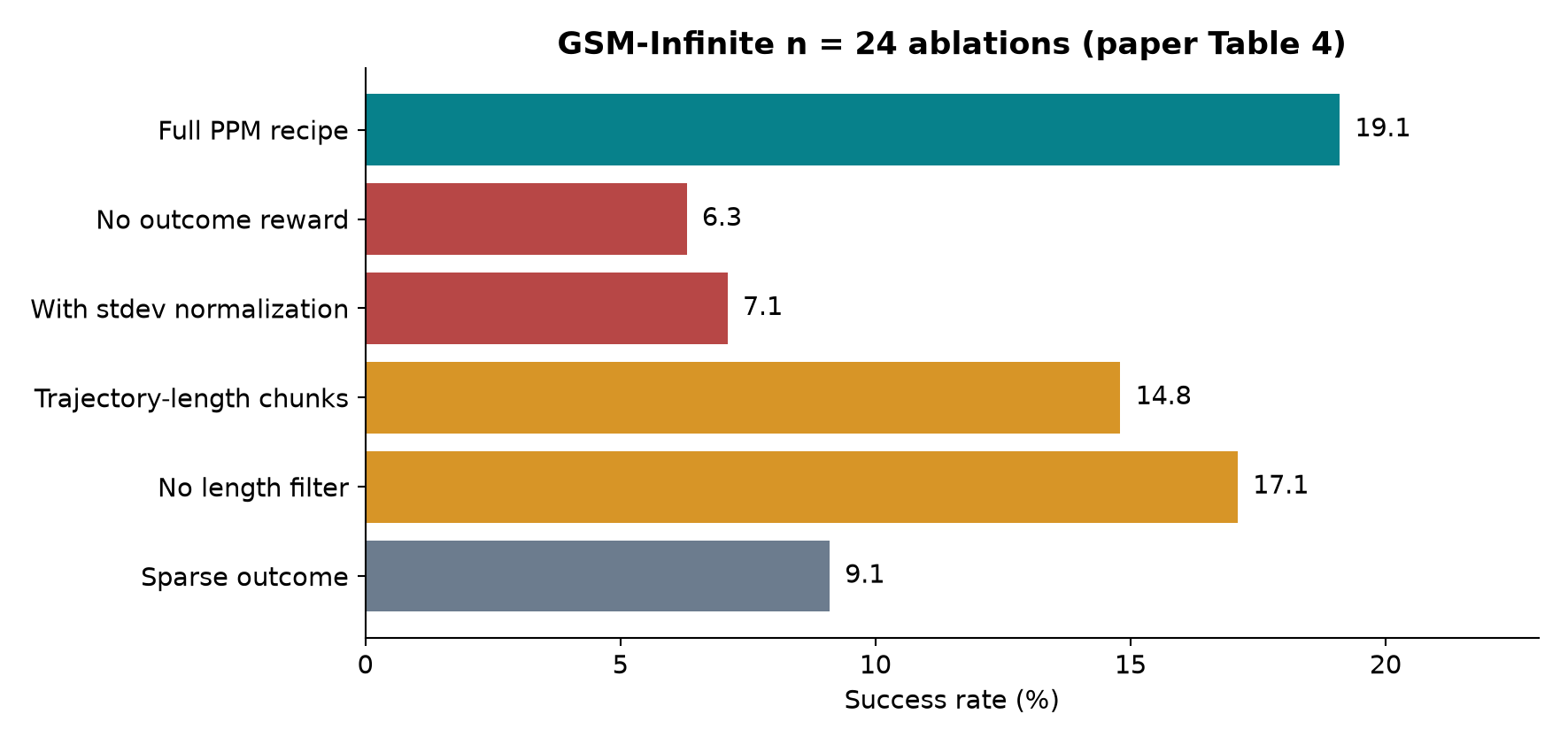
The outcome-reward ablation is the most important qualification to the high-level narrative. The ideal theorem explains when progress credit and final success share optimal policies. It does not establish that optimizing an imperfect progress signal alone is the best finite-compute recipe. The large empirical benefit of adding final reward shows that reliable completion feedback remains valuable. Conversely, POPE-hard uses PPM alone and still improves: the right mixture depends on whether successful outcomes are available during training.

The normalization result is also informative. Suppose a group has nearly identical progress rewards. Dividing by a tiny empirical standard deviation can turn a small distinction—possibly judge noise—into a large normalized advantage. Mean centering preserves the absolute reward gap. This is a plausible interpretation of the ablation, not a demonstrated causal explanation from a controlled noise study. A useful follow-up would vary judge disagreement and normalization jointly.

Fixed-budget chunks provide a comparable token coordinate across trajectories. With a 4,096-token limit and four chunks, boundaries occur every 1,024 tokens. A 2,400-token response occupies two complete chunks, one partial chunk and one empty chunk. Splitting each response into four equal fractions would instead use 600-token chunks. Then “segment three” would cover different absolute amounts of computation for short and long responses. Assigning group-centered advantages to such varying lengths can create unwanted incentives.

Truncation masking has a tradeoff. It reduces pressure to force an answer before the cap, but removes some expensive trajectories from gradient updates. Longer or harder examples may be disproportionately masked. The meaningful denominator is therefore not only generated tokens: one should also report retained tokens and retained trajectories by difficulty. These ablations should guide such measurements, rather than be interpreted as universally optimal settings.

9. Real math: extrapolation is promising, but mixed

9.1 Polaris-trained models

For Polaris, the authors train Qwen3-4B at an 8K token budget and evaluate at 16K. Their filtered preparation starts from 3,903 problems, removes items that cannot be easily verified to obtain 3,509, and then keeps 2,287 after generating usable oracle solutions, points and graphs. The paper specifies a training split with boxed-answer formatting. This is a selected dataset, not an untouched evaluation of all Polaris problems.

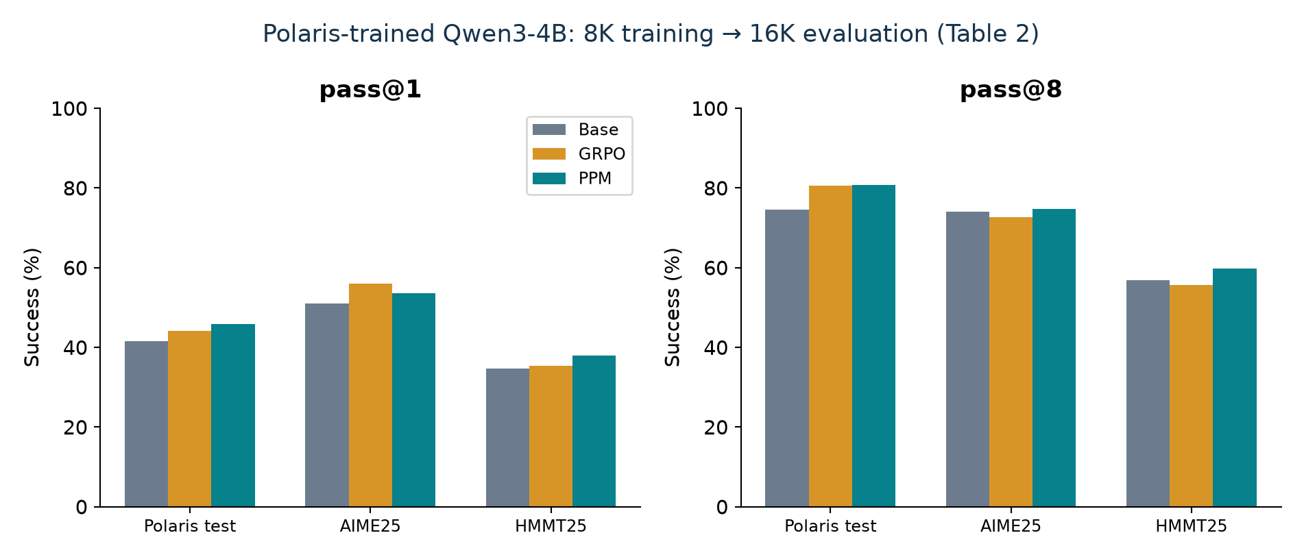
Evaluation metric	Base	GRPO	PPM
Polaris test pass@1	41.6%	44.1%	45.9%
Polaris test pass@8	74.5%	80.6%	80.7%
AIME25 pass@1	51.0%	56.0%	53.5%
AIME25 pass@8	74.0%	72.7%	74.8%
HMMT25 pass@1	34.6%	35.4%	37.9%
HMMT25 pass@8	56.9%	55.6%	59.8%

The Polaris test improvement over GRPO is 1.8 points at pass@1 and 0.1 points at pass@8. The latter is effectively a close result absent uncertainty estimates; it should not be advertised as a large gain. PPM trails GRPO on AIME25 pass@1 by 2.5 points. Table 2 also includes other baselines: Verifree reaches 46.1% Polaris test pass@1, and process rewards reach 83.2% pass@8, both above PPM on those metrics. PPM’s HMMT25 results are stronger in the reported table.

SFT has an especially different profile: 60.9% train pass@8, but only 65.1% Polaris test pass@8 and 9.8% AIME25 pass@1. The paper trains this baseline on reference solutions in non-thinking mode. This is relevant evidence about that setup’s transfer, not proof that every supervised warm start or every teacher-trace dataset would fail similarly.

9.2 Near-zero-reward POPE-hard

The selected POPE-hard subset is more directly aligned with the motivation. From 2,515 source problems, 601 have zero observed success over 16 unguided samples at 8K; the final 0p10p subset contains 382 of these for which a ten-paragraph oracle prefix makes some successes observable. All paper references to POPE-hard refer to that final subset. It is selected to contain difficult but guidance-responsive problems.

At 4K training and 16K evaluation, GRPO matches the base model at 0.4% pass@1 and 2.3% pass@8. POPE reaches 1.2% and 6.3%; PPM reaches 3.5% and 14.8%. Thus the pass@8 gain over POPE is 8.5 percentage points, about 2.35×. These remain low absolute success rates: most sampled attempts still fail, even after improvement.

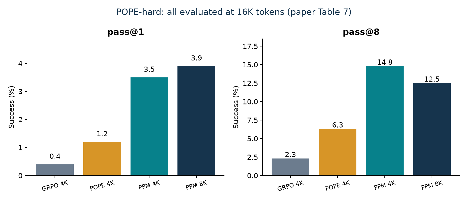
At 8K training, PPM gives 3.9% pass@1 and 12.5% pass@8 at 16K evaluation. The authors hypothesize that intermediate length pressure encourages early guessing and shorter outputs. The 4K model may learn intermediate progress without trying to complete an effectively impossible task inside the training cap. The experiment motivates this explanation, but does not establish it as the unique cause.

The shortcutting ablation is also nuanced. At 4K training, removing shortcutting reduces test pass@8 from 14.8% to 9.3%. At 8K training it yields 11.7% versus 12.5%, while pass@1 is actually 4.1% without shortcutting versus 3.9% with it. Exact-order point matching is much worse. The evidence favors flexibility over rigid reference order, while still leaving individual metrics where a restricted variant does well.

9.3 Read pass@k as a coverage measure

For a single prompt with independent sample success probability $q$, pass@k is $1-(1-q)^k$. When evaluation draws $M$ responses and observes $c$ successes, Appendix B uses the standard estimator

$$\widehat{\mathrm{pass@}k}=1-\frac{\binom{M-c}{k}}{\binom{M}{k}}.$$

The numerator counts all-failure subsets of size $k$; the denominator counts all such subsets. Subtracting their ratio from one gives the chance that a random subset contains at least one correct answer. The reported metric averages this per-prompt quantity. It is not generally correct to insert the dataset’s mean pass@1 into $1-(1-q)^k$, because prompts have different success probabilities and the transformation is nonlinear.

The POPE-hard 4K/8K ranking difference could reflect changed coverage across prompts, changed sampling diversity, or both. It cannot be uniquely diagnosed from two aggregate metrics. Per-prompt success distributions, response lengths and repeated seeds would help distinguish these mechanisms. A high pass@8 additionally presumes some way to recognize success among samples; it does not by itself deliver a reliable single final answer to an end user.

10. Judges, references and total cost

10.1 Judge evaluation is encouraging but small

The paper uses gemini-2.5-flash-lite for PPM and process judging, with points and graphs generated using Gemini 3 Flash variants. It evaluates whether judge scores respond sensibly to increasingly helpful reference prefixes. Section 5.3 reports Kendall rank correlation 0.856 for the PPM prompt versus 0.768 for a standard rubric prompt. Appendix B.3 describes a probe with eight prompts, five reference-prefix conditions and eight continuations per condition, and shows similar score trends across several judge models.

A ranking correlation is useful, but it is not a calibrated probability-of-success guarantee. More reference text can raise both judge scores and continuation success, without establishing that the same relationship holds on policy-generated erroneous prefixes. The claim that a useful progress score should grow approximately linearly with future success is best treated as a calibration heuristic, not a general theorem. With heterogeneous remaining subproblems, equal increments in reference coverage need not imply equal increments in completion probability.

Tables 5 and 6 evaluate point extraction and reasoning graphs. In v1, the numerical entries in those two tables are identical, despite describing different measurements. I would ask the authors to confirm whether this is intentional or a reporting duplication. The point-recall experiment also uses only 32 held-out prompts. High recall on such examples does not measure false positive points, irrelevant dependencies or robustness to alternative correct solution routes.

10.2 Prefix scoring multiplies judge input

Let a response use $L$ tokens and let $H$ denote the repeated problem, rubric and prompt overhead. Scoring $K$ uniformly spaced full prefixes requires approximately

$$\begin{aligned} T_{\mathrm{judge,input}} &=\sum_{k=1}^{K}\left(H+\frac{kL}{K}\right)\\ &=KH+\frac{K+1}{2}L. \end{aligned}$$

For four chunks, this is $4H+2.5L$, before judge output tokens, retries or caching. If $L=4096$ and $H=1000$ in an illustrative calculation, judge input totals 14,240 tokens. These are token counts, not equal-cost units: prefill, policy generation and training have different hardware efficiencies and prices. The paper notes that judging is largely prefill and that point/graph generation is performed once per dataset. Both help amortization, but neither makes this cost zero.

A complete comparison should hold an end-to-end budget fixed:

$$C_{\mathrm{total}}=C_{\mathrm{reference}}+C_{\mathrm{points/graphs}} +C_{\mathrm{rollout}}+C_{\mathrm{judge}}+C_{\mathrm{update}}.$$

The training-token plots establish a useful efficiency axis. They do not by themselves establish that PPM beats outcome-only training at equal wall-clock time, dollar cost or energy after accounting for external judgments. Sharing prefixes, caching reference material, batching judges and using smaller validated judges are plausible ways to reduce cost, but their benefit must be measured.

10.3 Reference granularity is a design variable

Many tiny points approach detailed imitation: easier matching, more opportunities for feedback, but greater dependence on a particular derivation. A single final point recovers outcome-only learning and loses intermediate signal. Good intermediate points should be sufficiently meaningful to support future work while allowing multiple ways to reach them.

Point density also controls incentives. A reference with ten trivial algebraic rewrites and one decisive insight distributes credit differently from a reference with one point for the setup and one for the insight. Normalizing by the number of points does not remove this difference. A useful evaluation would compare alternative decompositions of the same reference, not only different judge model sizes.

11. Design choices and where alternatives make sense

Choice	Why it helps	Alternative and failure boundary
Points rather than verbatim traces	Allows different wording and routes	Direct distillation can be simpler when expert behavior is exactly desired
Shortcutting	Avoids penalizing valid shorter solutions	Overbroad closure can award unsupported results
Full-prefix judging	Keeps definitions and context	Local checking is cheaper when steps are independently verifiable
Four fixed-budget chunks	Localizes credit with moderate judge calls	Too-coarse chunks blur credit; too-fine chunks raise cost and noise
Mean-only normalization	Retains absolute reward distinctions	Standardization can help scale invariance but amplify tiny noisy gaps
Truncation masking	Reduces completion pressure	Can remove precisely the hardest useful trajectories

The paper’s three budget regimes are a useful organizing hypothesis. Very short training budgets make completion unavailable; intermediate budgets may invite premature guesses; sufficiently long budgets allow completion to dominate. A single training length need not place every problem in the same regime. Mixing difficulty levels means mixing these incentives within a batch.

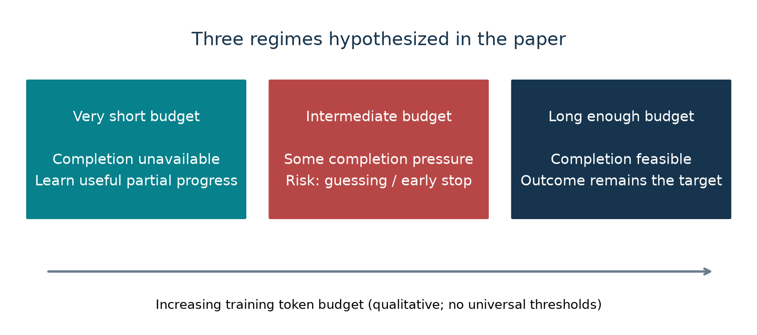
For a proposed follow-up, I would stratify problems by observed partial progress and completion frequency, then compare budget policies within each stratum. This would test whether short-budget training helps because of reduced length pressure, a more favorable compute allocation, or a different set of retained trajectories after filtering. It would also distinguish useful horizon extrapolation from merely exploiting an evaluation budget that every baseline benefits from.

12. Limitations of the present evidence

Scale and task range. Experiments focus on 1.7B and 4B models, synthetic environments and selected mathematics. The introduction’s motivation includes tasks lasting hours or days, but the experiments do not establish reliable autonomous coding, irreversible tool use or multi-day task completion. Moving from text reasoning to changing external environments breaks several convenient assumptions.

Reference availability. The learner needs a useful solution for each training problem, even when it cannot solve the problem itself. Oracle generation and filtering can reject the hardest or most ambiguous cases. The result is an important way to exploit privileged information, but not evidence that the system can learn entirely novel unsolved tasks without a source of progress labels.

Approximate state and judge. Reachability is represented by textual evidence and inferred relations. The set abstraction is monotone, whereas an LLM’s actual ability to continue can deteriorate when its context becomes long or contradictory. A point can remain present in text yet become functionally unusable. Semantic grading errors, graph errors and policy adaptation to the rubric all complicate the guarantee.

Statistical resolution. Main tables do not supply uncertainty intervals for every comparison. Differences such as 80.7% versus 80.6% pass@8 cannot sustain a strong superiority claim without repeated runs or paired uncertainty estimates. Very low-success subsets need especially careful reporting of sample counts and prompt-level variation.

Training versus generalization. POPE-hard demonstrates learning under near-zero outcome feedback and evaluation at a larger token budget on the described hard problem set. This is valuable, but budget extrapolation and generalization to unseen problem distributions are distinct. The selected 382-problem subset also favors problems responsive to oracle guidance. Claims should retain that selection condition.

Recipe dependence. Outcome mixing is crucial on GSM-Infinite yet omitted in the POPE-hard PPM setup. Chunking, standardization and filtering all affect the result. An appealing theorem does not eliminate the need to specify those practical decisions when interpreting experimental gains.

13. Critical Analysis: what would make the case stronger

13.1 The ideal reward and the supplied graph prompt are not the same contract

The most consequential discrepancy is textual. Section 4’s ideal construction says the goal makes all reference points reached. Appendix D’s graph-generation prompt tells the generator not to let a final answer obsolete substantive derivations, constructions, case analyses or impossibility arguments. Its example nevertheless includes local obsoletion chains leading back from a conclusion. A generated graph may therefore or may not give every successful alternative full closure.

This does not establish that the experiments are invalid. It establishes that the theoretical shortcut property cannot be inferred from the prompt alone. A clean paper-level test would present multiple independently valid solutions to the same problem, including shorter routes that omit reference lemmas, and report whether each receives full terminal credit. The final verifier should decide actual success separately from rubric overlap. The same probe should include bare answer guesses and unsupported intermediate claims, because permissive shortcutting and rigorous evidence requirements pull in opposite directions.

13.2 Separate signal quality from changing the objective

PPM is attractive precisely because it changes the treatment of unsuccessful trajectories. It assigns them different values. Therefore the improvement may combine lower variance, better exploration incentives, reference-derived curriculum and a changed transient objective. The SNR analysis isolates a particular stylized part of that story; it does not isolate all of these factors in the neural experiments.

A more decisive experiment would compare immediate segment credit, reward-to-go, trajectory PPM and an outcome-plus-shaping construction with matched reward scale and identical judge calls. It would report their effect on outcome success rather than only the shaped reward. That design would reveal which gain comes from exposing partial information and which comes from a particular gradient estimator. It would also make the relationship between Algorithm 1’s abstract advantage function and Appendix A’s local estimator explicit.

13.3 Test the judge where the policy is likely to exploit it

Reference-prefix interpolation is a reasonable initial calibration probe. It is an easy distribution relative to the policy’s most problematic outputs: a prefix copied from a valid reference is unusually coherent. A stronger evaluation should include contradictory prefixes, recycled lemmas, right intermediate numbers from wrong reasoning, and alternative valid proofs. Judge recall alone is insufficient; the false-credit rate matters because optimization can concentrate on the examples that fool it.

The monotone set formulation also raises a question about changing state: when a longer prefix contradicts an earlier result, should the earlier point stay credited? For abstract mathematical knowledge, retaining it may be defensible. For an agent that has overwritten a file or consumed a resource, it may be false. The reward definition should explicitly distinguish accumulated evidence from the current validity of an external state before extending PPM to agents.

13.4 Use a budget that includes the teacher and the judge

The question for a training team is whether the same total resources could obtain better outcomes through more rollouts, better reference data, a learned critic, or more PPM judgments. An equal policy-token plot omits costs that differ substantially across those options. I would want a frontier of final-answer accuracy versus total spend, with reference construction amortized over a stated number of training uses.

Report judge calls, input/output tokens, caching assumptions, retained rollout fraction and latency as separate quantities. Such a report could still favor PPM strongly. It would simply make the engineering conclusion comparable to the theoretical and token-efficiency conclusions, rather than treating them as interchangeable.

13.5 A compact next-study design

Algorithm 3. Proposed evaluation study (not performed here)
1. Freeze disjoint training, development and unseen-problem sets.
2. Create several valid reference decompositions per training item.
3. Validate goal closure and false-credit rates on held-out traces.
4. Compare reward assignments at matched total training cost.
5. Sweep training length, judge model and chunk count separately.
6. Evaluate at multiple lengths with outcome pass@1 and pass@k.
7. Report repeated seeds, prompt-level intervals and retained data.
8. Inspect failures by graph structure and reference-route mismatch.

This study addresses PPM’s distinctive uncertainty: whether a compact, trustworthy progress measure can continue to guide exploration when the policy leaves the reference path. It would be more informative than another aggregate leaderboard score at one length.

14. Conclusion

PPM provides a clear way to turn a reference solution into partial on-policy learning signal. Its key contribution is the combination of progress increments, localized credit and shortcutting, supported by a graph-based SNR analysis and controlled horizon experiments. The near-zero-reward math results make a persuasive case that useful learning can occur before final answers become common.

The practical conclusion is conditional. The optimal-policy guarantee assumes ideal reachability and sufficient ability to complete the task; judges and inferred graphs only approximate that setting. Real benchmark gains are mixed, and external judging cost remains part of the tradeoff. For long-horizon RL, PPM is a strong research direction for making failures informative, provided that final success, alternative valid routes and total cost remain the evaluation targets.

References and figure provenance

1. Fu, P., Frans, K., Rybkin, O., Levine, S., and Kumar, A. Long-Horizon Language Model Reinforcement Learning via Progressive Point Matching, 2026. Primary source for all reported experimental results, algorithms, propositions and appendix observations.
2. PPM author explanation and official resource entry. The linked repository is provided as a resource.
3. Qu, Y., Setlur, A., Smith, V., Salakhutdinov, R., and Kumar, A. POPE: Learning to Reason on Hard Problems via Privileged On-Policy Exploration. Related reading for guided exploration; today’s POPE comparison numbers are from PPM Table 7.
4. Cheng, Z., et al. IsoCompute Playbook: Optimally Scaling Sampling Compute for LLM RL. Related reading for sampling-budget allocation.

Figures 1–3 and 9 are original explanatory diagrams. Figure 4 evaluates the explicitly stated toy-model moments. Figures 5–8 redraw selected values from PPM Tables 1, 4, 2 and 7, respectively. Percentage-point changes and ratios in the text are arithmetic on those tables. No additional model-training experiment is claimed.